The answer to the first question just posed is extremely simple – the internal propagators connecting MHV vertices are simply scalar propagators, $i/(L^{2}+i\varepsilon)$. This result can be justified from the Lagrangian formulation of MHV rules described in [12]. Next, we consider the issue of off-shell continuation. Let $L$ be an internal (hence off-shell) momentum. The MHV amplitude depends on the holomorphic spinors associated to the external, on-shell particles, and we will now provide a prescription that associates a spinor to the internal leg with (off-shell) momentum $L$. To this end, one introduces an arbitrary lightlike reference vector $\eta_{\alpha{\dot{\alpha}}}=\eta_{\alpha}\tilde{\eta}_{{\dot{\alpha}}}$. Then, there is a unique way to decompose $L$ as [7, 31]

$$L\ =\ l\,+\,z\eta\ ,$$

(2.6)

where $l:=\lambda_{L}\tilde{\lambda}_{L}$ is a null momentum and $z$ is a real parameter, which can easily be seen to be equal to $z=L^{2}/(2L\cdot\eta)$. The off-shell continuation proposed in [2] consists in using the spinor $\lambda_{L}$ as the off-shell continuation for the internal leg of momentum $L$. It then follows that

$\displaystyle\lambda_{L,\alpha}$

$\displaystyle=$

$\displaystyle{L_{\alpha{\dot{\alpha}}}\tilde{\eta}^{{\dot{\alpha}}}\over[\tilde{\lambda}_{L}\,\tilde{\eta}]}\ .$

(2.7)

These equations coincide with the prescription originally proposed in [2] by CSW for determining the spinor variable $\lambda_{L}$ associated with the off-shell (i.e. non-null) four-vector $L$ defined in (2.6). The denominators arising from the right-hand side of (2.7) will be irrelevant for our applications, since each MHV diagram is invariant under rescalings of the internal spinor variables; hence we will discard them and simply replace $\lambda_{L,\alpha}\to L_{\alpha{\dot{\alpha}}}\tilde{\eta}^{{\dot{\alpha}}}$. Each MHV diagram will therefore depend on the particular choice of $\tilde{\eta}$; one will then have to prove that summing over all MHV diagrams, this spurious dependence cancels, showing that the MHV diagrams produce covariant answers. In [2] this was originally shown for diagrams involving one propagator i.e. NMHV gluon amplitudes. Later an elegant proof was found in [32] where it was shown that MHV diagrams are in direct correspondence with on-shell recursion relations (which by construction lead to covariant answers and will be described in later sections) where all negative helicity gluons are shifted. This was later extended to include all tree amplitudes in ${\cal N}=4$ SYM [33].

The proposal of [2] that tree amplitudes could be built by gluing together MHV tree amplitudes as vertices, joining them with propagators, was very intuitive and gave an answer to the basic question of how tree amplitudes for $n$-particle scattering could be relatively simple, when they were obtained by summing a rapidly increasing number of Feynman diagrams. This method promised a new, efficient means for calculating amplitudes, seemingly sidestepping the complications of gauge fixing and dealing with unwieldy sets of diagrams.

We will start with some simple applications at tree level and defer the more complicated example of all NMHV tree amplitudes for later where we will combine the CSW rules with Nair’s on-shell superspace formalism.

As a warm-up we will now rederive the well-known fact that the four-point tree amplitude $\langle 1^{+}2^{-}3^{-}4^{-}\rangle$ vanishes. More generally, all trees with equal helicity gluons or only a single gluon of opposite helicity are zero. A very important exception to this are the three-point amplitudes $\langle 1^{+}2^{-}3^{-}\rangle$ and $\langle 1^{-}2^{+}3^{+}\rangle$ which vanish for real momenta in Minkowski signature but are non-vanishing for complex momenta (as we will see later, this has profound consequences). Formally, our example is a so-called next-to-MHV (NMHV) amplitude, as it has three negative helicity gluons.

There are two diagrams contributing to this amplitude, where two three-point MHV vertices are connected by a propagator, see Figure 1.

Using the fact that $P^{2}=(p_{1}+p_{2})^{2}=\langle 12\rangle[21]$ and $P^{\prime 2}=(p_{1}+p_{4})^{2}=\langle 14\rangle[41]$ we obtain for the sum of the two diagrams,

$$i^{3}\frac{\langle 2P\rangle^{3}}{\langle P1\rangle\langle 12\rangle}\frac{1}{\langle 12\rangle[21]}\frac{\langle 34\rangle^{3}}{\langle 4\,-\!\!P\rangle\langle-\!P3\rangle}+i^{3}\frac{\langle 23\rangle^{3}}{\langle 3-\!\!P^{\prime}\rangle\langle-\!P^{\prime}2\rangle}\frac{1}{\langle 14\rangle[41]}\frac{\langle P^{\prime}4\rangle^{3}}{\langle 41\rangle\langle 1P^{\prime}\rangle}\,.$$

(2.8)

Now we have to use the off-shell continuation introduced earlier namely $\lambda_{P,\alpha}=P_{\alpha\dot{\alpha}}\tilde{\eta}^{\dot{\alpha}}=-i\lambda_{-\!P,\alpha}$, and we have denoted incoming internal momenta with an additional minus sign since they correspond to an outgoing momentum $-P$. In our convention for on-shell momenta, $p_{\alpha\dot{\alpha}}:=\lambda_{\alpha}\tilde{\lambda}_{\dot{\alpha}}$, whenever we flip the orientation from outgoing to incoming we multiply $\lambda$ and $\tilde{\lambda}$ with $i$. Taking into account these extra factors of $i$ and using the off-shell continuation we get, for the first diagram²² 2 Note that, as we mentioned earlier, we are allowed to drop the normalisation constant in the definition of the off-shell continuation since (2.9) is homogeneous in the internal off-shell spinors – this is a generic feature of MHV diagrams.

$$i\frac{\langle 2|P|\eta]^{3}\langle 34\rangle^{3}}{[\eta|P|1\rangle\langle 12\rangle^{2}[21]\langle 4|P|\eta][\eta|P|3\rangle}=i\frac{\langle 34\rangle}{[21]}\frac{[1\eta]^{3}}{[2\eta][3\eta][4\eta]}\,,$$

(2.9)

where we used $P=-p_{1}-p_{2}=p_{3}+p_{4}$ and identities such as $\langle 2|P|\eta]=\langle 2|-p_{1}-p_{2}|\eta]=-\langle 21\rangle[1\eta]-\underbrace{\langle 22\rangle}_{=0}[2\eta]=\langle 12\rangle[1\eta]$. The evaluation of the second diagram gives

$$i\frac{\langle 14\rangle}{[23]}\frac{[1\eta]^{3}}{[2\eta][3\eta][4\eta]}\,.$$

(2.10)

The sum of (2.9) and (2.10) vanishes, since

$$\frac{\langle 34\rangle}{[21]}+\frac{\langle 14\rangle}{[23]}=\frac{[23]\langle 34\rangle+[21]\langle 14\rangle}{[21][23]}=\frac{[2|p_{3}+p_{1}|4\rangle}{[21][23]}=-\frac{[2|p_{2}+p_{4}|4\rangle}{[21][23]}=0\ ,$$

(2.11)

confirming that the $\langle 1^{+}2^{-}3^{-}4^{-}\rangle$ amplitude is indeed zero.

This procedure can be easily generalised to calculate arbitrary $n$-point amplitudes with $k$ negative helicity gluons. Such N^k-2MHV amplitudes require one to sum all possible MHV diagrams with $k-1$ MHV vertices connected by scalar propagators. Applications are not restricted to amplitudes with gluons only but can also involve fermions or scalars [34, 35].

An obvious next step was to see if this method could be used to calculate loop amplitudes and we would like to briefly describe how this is achieved [8]. Much was already known about loop amplitudes, particularly after work using unitarity methods in the 1990’s [36, 37, 38, 39, 40, 41]. Applications of modern unitarity techniques are discussed in great detail in the chapters of this review by Britto [42] and Bern and Huang [43].

The first and simplest example of a loop amplitude is the one-loop MHV amplitude in the ${\cal N}=4$ theory, which is given as sum over “two-mass easy box functions”[44]. Explicitly, one has [36]

$$A_{n;1}^{{\cal N}=4\,{\rm MHV}}=A^{\rm tree}_{n}\,\sum_{i=1}^{n}\sum_{r=1}^{[{n\over 2}]-1}\Bigl(1-{1\over 2}\delta_{{n\over 2}-1,r}\Bigr)\,F_{n:r;i}^{2m\,e}\ .$$

(2.12)

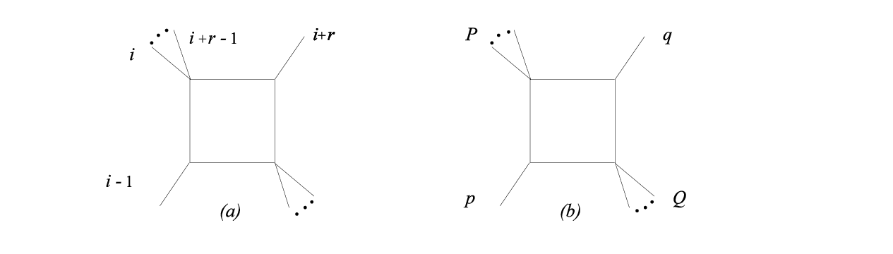
In order to define the two-mass easy box functions $F^{2me}$, we first introduce the scalar box integral $I_{4}$, defined as

$$I_{4}=-i(4\pi)^{2-\epsilon}\,\int\frac{d^{4-2\epsilon}p}{(2\pi)^{4-2\epsilon}}\,\,\frac{1}{p^{2}(p-K_{1})^{2}(p-K_{1}-K_{2})^{2}(p+K_{4})^{2}}\ .$$

(2.13)

In the two-mass easy case, two opposite momenta in the box integral are massless ($p$ and $q$ in Figure 2 (b)), and the remaining two opposite momenta are massive ($P=k_{i}+\dots+k_{i+r-1}$ and $Q=k_{i+r+1}+\dots+k_{i+n-2}$ in the same figure). Denoting by $I_{4:r;i}^{2m\,e}$ the two-mass easy box integrals, the corresponding $F$ functions are defined by

	$\displaystyle I_{4:r;i}^{2m\,e}$	$\displaystyle=$	$\displaystyle-\frac{2F_{n:r;i}^{2m\,e}}{t^{[r+1]}_{i-1}t^{[r+1]}_{i}-t^{[r]}_{i}t^{[n-r-2]}_{i+r+1}}\ ,$
	$\displaystyle I_{4:i}^{1m}$	$\displaystyle=$	$\displaystyle-\frac{2F_{n:i}^{1m}}{t^{[2]}_{i-3}t^{[2]}_{i-2}}\ ,$		(2.14)

where $t_{i}^{[r]}=(k_{i}+\dots+k_{i+r-1})^{2}$ are the kinematic invariants constructed from sums of cyclically adjacent external momenta. Note that $P^{2}=t^{[r]}_{i}$ and $Q^{2}=t^{[n-r-2]}_{i+r+1}$. In the second equation in (2.14) we have considered separately the one-mass case, i.e. the special case where one of the two massive corners $P$ or $Q$ becomes massless. The corresponding function is obtained as a smooth limit of the two-mass easy configuration [44]. Introducing the variables

$$s\ :=\ (P+p)^{2}=t^{[r+1]}_{i-1}\ ,\qquad t\ :=\ (P+q)^{2}=t^{[r+1]}_{i}\ ,$$

(2.15)

the explicit expression of the box function is [36]

	$\displaystyle F(s,t,P^{2},Q^{2})$	$\displaystyle:=$	$\displaystyle-{1\over\epsilon^{2}}\Bigl[(-s)^{-\epsilon}\,+\,(-t)^{-\epsilon}\,-\,\big((-P)^{2}\bigr)^{-\epsilon}\,-\,\big((-Q)^{2}\bigr)^{-\epsilon}\Bigr]$		(2.16)
		$\displaystyle+$	$\displaystyle{\rm Li}_{2}\Bigl(1-{P^{2}\over s}\Bigr)\,+\,{\rm Li}_{2}\Bigl(1-{P^{2}\over t}\Bigr)+{\rm Li}_{2}\Bigl(1-{Q^{2}\over s}\Bigr)\,+\,{\rm Li}_{2}\Bigl(1-{Q^{2}\over t}\Bigr)$
		$\displaystyle-$	$\displaystyle{\rm Li}_{2}\Bigl(1-{P^{2}Q^{2}\over s\,t}\Bigr)\,+\,{1\over 2}\log^{2}\Bigl({s\over t}\Bigr)\ ,$

where $P+p+Q+q=0$. The relation to the functions $F_{n:r;i}^{2m\,e}$ is obtained by setting $p=p_{i-1}$, $q=p_{i+r}$, and $P=p_{i}+\cdots+p_{i+r-1}$.

Following the CSW proposal discussed above, one would immediately expect that the one-loop MHV amplitude should arise from the one-loop MHV diagrams depicted in Figure 3 below, i.e. from gluing two MHV vertices together with two propagators in order to form a one-loop diagram, and summing all possible diagrams while preserving the cyclic ordering of the external legs.

This calculation was performed in [8]. One important point to discuss is the loop integral measure,

$$d{\cal M}\ :=\ {d^{4}L_{1}\over L_{1}^{2}+i\varepsilon}\,{d^{4}L_{2}\over L_{2}^{2}+i\varepsilon}\ \delta^{(4)}(L_{2}-L_{1}+P_{L})\ ,$$

(2.17)

where $L_{1}$ and $L_{2}$ are loop momenta, and $P_{L}$ is the external momentum flowing outside the loop³³ 3 In our conventions, all external momenta are outgoing. so that $L_{2}-L_{1}+P_{L}=0$. Note that we also include the two propagators in the definition of the integration measure for convenience.

In order to calculate the one-loop MHV diagram in Figure 3, we need to re-express a standard loop momentum in terms of the new variables $l$ and $z$ introduced in (2.6). One finds that [8]

$${d^{4}L\over L^{2}}\ =\ d{\cal N}(l)\,{dz\over z}\ ,$$

(2.18)

with the Nair measure [25]

$$d{\cal N}(l):=\,\langle l\,\,dl\rangle\,d^{2}\tilde{l}\ -\ [\tilde{l}\,\,d\tilde{l}]\,d^{2}l\ .$$

(2.19)

Note that the product of the measure factor with a scalar propagator $d^{4}L/L^{2}$ of (2.18) is independent of the reference vector $\eta$. Also, the Lorentz invariant phase space measure for a massless particle can be expressed precisely in terms of the Nair measure:

$$d^{4}l\,\delta^{(+)}(l^{2})\ =\ {d{\cal N}(l)\over 4i}\ ,$$

(2.20)

where, as before, we write the null vector $l$ as $l_{\alpha{\dot{\alpha}}}=l_{\alpha}\tilde{l}_{{\dot{\alpha}}}$, and in Minkowski space we identify $\tilde{l}=\pm l^{\ast}$ depending on the sign of the energy.

We are now in position to write the one-loop integration measure in terms of variables that are appropriate for the MHV diagram method. Expressing $L_{1}$ and $L_{2}$ as in (2.6),

$$L_{i;\alpha,{\dot{\alpha}}}\ =\ l_{i\alpha}\tilde{l}_{i{\dot{\alpha}}}\,+\,z_{i}\,\eta_{\alpha}\tilde{\eta}_{{\dot{\alpha}}}\ ,\qquad i=1,2\ ,$$

(2.21)

we rewrite the argument of the delta function in (2.17) as

$$L_{2}-L_{1}+P_{L}=l_{2}-l_{1}+P_{L;z}\ ,$$

(2.22)

where $P_{L;z}:=P_{L}-z\eta$, and $z\ :=\ z_{1}\,-\,z_{2}$. Notice that we use the same $\eta$ for both the momenta $L_{1}$ and $L_{2}$. Using (2.21), we can re-cast (2.17) as [8]

$$d{\cal M}\ =\ {dz_{1}\over z_{1}+i\varepsilon_{1}}\,{dz_{2}\over z_{2}+i\varepsilon_{2}}\ \bigg[{d^{3}l_{1}\over 2l_{10}}\,{d^{3}l_{2}\over 2l_{20}}\,\delta^{(4)}(l_{2}\,-\,l_{1}\,+\,P_{L;z})\bigg]\ ,$$

(2.23)

where $\varepsilon_{i}:={\rm sgn}(\eta_{0}l_{i0})\varepsilon={\rm sgn}(l_{i0})\varepsilon$, $i=1,2$ (the last equality holds since we are assuming $\eta_{0}>0$).

The next step involves integrating out the variable $z^{\prime}:=z_{1}+z_{2}$, which only appears through the integration measure

$${dz_{1}\over(z_{1}+i\varepsilon_{1})}\,{dz_{2}\over(z_{2}+i\varepsilon_{2})}:=2\,{dz\,dz^{\prime}\over\big[(z^{\prime}+z+i\varepsilon_{1})(z^{\prime}-z+i\varepsilon_{2})\big]}\ .$$

(2.24)

This can be done using the residue theorem, with the result [8, 45] that one can simply replace

$${dz_{1}\over(z_{1}+i\varepsilon_{1})}\,{dz_{2}\over(z_{2}+i\varepsilon_{2})}\ \rightarrow\ 2\pi i\,{dz\over z+i\varepsilon}\ .$$

(2.25)

The last crucial step consists in performing the integration over $z$. Perfectly in tune with the S-matrix programme, this was converted in [8] into a dispersion integral. The final result for the integration is then [8, 45]

$$d{\cal M}\ =\ 2\pi i\ \theta(P_{L;z}^{2})\ {dP_{L;z}^{2}\over P_{L;z}^{2}\,-\,P_{L}^{2}\,-\,i\varepsilon}\ d{\rm LIPS}(l_{2}^{\mp},-l_{1}^{\pm};P_{L;z})\ ,$$

(2.26)

where

$$d{\rm LIPS}(l_{2}^{-},-l_{1}^{+};P_{L;z})\ :=\ d^{4}l_{1}\,\delta^{(+)}(l_{1}^{2})\ d^{4}l_{2}\,\delta^{(-)}(l_{2}^{2})\ \delta^{(4)}(l_{2}-l_{1}+P_{L;z})\$$

(2.27)

is the two-particle Lorentz invariant phase space (LIPS) measure, and we recall that $\delta^{\pm}(l^{2}):=\theta(\pm l_{0})\delta(l^{2})$.

It is important to observe that the integration is performed for $P_{L;z}^{2}>0$. By setting all the various external kinematical invariants $P_{L}^{2}$ to negative values, no poles are encountered along the integration contour and the $i\varepsilon$ prescription can be dropped. However, (2.26) provides us with the correct analytic continuation to the physical region, which is obtained by simply performing the substitution $P^{2}_{L}\ \longrightarrow\ P^{2}_{L}\,+\,i\varepsilon$.

Having fully re-expressed the integration in terms of MHV variables, one can now perform all the remaining integrations and sum over all possible MHV diagrams corresponding to the different choices of particles running in the internal legs on each of the two MHV vertices. The interested reader can consult [8] for the remaining part of the calculation; in the following we will outline its main steps.

Firstly, one finds that each MHV diagram leads to a sum of four terms which are written as dispersion integrals in the channel fixed by the diagram. These are related to unitarity cuts of four different box functions. Crucially, in order to reconstruct complete box functions one has to take an appropriate combination of four dispersion integrals from four different MHV diagrams (channels). Surprisingly, it was found in [8] that dependence on the reference spinor $\eta$ cancels out between the four dispersion integrals contributing to a single box function and not only in the sum over all diagrams. The covariance at one-loop for arbitrary amplitudes was later shown in [45] using the Feynman tree theorem. Collecting all the box functions, one finds precisely the expected result (2.12).

We would like to make a few comments before closing this subsection.

Firstly, the CSW approach, and hence the general MHV diagram proposal for calculating scattering amplitudes, was originally motivated by the twistor space localisation of amplitudes and Witten’s formulation of ${\cal N}=4$ super Yang-Mills theory as a theory in twistor space. At first sight, then, one might not expect these methods to work for theories with less supersymmetry (at tree level of course the gluon scattering amplitudes are the same for the supersymmetric and non-supersymmetric cases). Nevertheless, one could just put aside considerations of the twistor picture, and simply see if the MHV diagrams do yield the correct amplitudes in Yang-Mills theories with less than maximal supersymmetry. This was done in [9, 10], where results from the MHV diagram calculation in ${\cal N}=2$ and ${\cal N}=1$ super Yang-Mills were found in agreement with those derived in [37] using unitarity. This success was somewhat unexpected, and led to a new, simpler understanding of the twistor space localisation of loop amplitudes in these theories [46, 47]. We also point out that this success was not accidental. Indeed, in [45] it was proved that any non-MHV amplitude in supersymmetric gauge theories is reproduced correctly by MHV diagrams.

Finally, the non-supersymmetric Yang-Mills theory was studied at one loop using MHV methods [11]. Again, this correctly yielded the (cut-constructible part of the) amplitude, and this work was notable in that it included the first calculation of a previously unknown amplitude using these methods. It was at this point that the issue of so-called rational terms arose – these are terms in amplitudes that are not generated by unitarity cuts performed in four dimensions. This problem is not present in supersymmetric Yang-Mills theories, but does appear in the non-supersymmetric theory. The MHV diagram approach, as used in [11], reproduced correctly all the non-rational terms, but not the rational ones. Note however that the MHV vertices that one inserts into the diagrams are essentially four-dimensional objects, although one does use dimensional regularisation in the loop integral; it is expected that it is this fact that underlies the missing rational pieces, although this remains to be investigated fully. Calculation of the rational terms has been achieved by various methods that are detailed e.g. in the chapter of this review from Britto [42].

It is generally the case that formalisms where symmetries are explicit are more powerful both conceptually and for calculations. It is easy to generalise MHV diagrams in ${\cal N}=4$ SYM to a manifestly supersymmetric version. This is particularly convenient when one is interested in amplitudes with external fermions or scalars. The on-shell superamplitude formalism introduced in the following is also reviewed in the chapter by Elvang, Freedman and Kiermaier [48].

The ${\cal N}=4$ theory contains two gluons $G^{\pm}(p)$ with helicities $1,-1$, four fermions $\psi_{A}$ of helicity $+1/2$, transforming in the fundamental of the R-symmetry group $SU(4)_{\mathrm{R}}$ of the ${\cal N}=4$ theory, four Weyl fermions $\bar{\psi}^{A}$ with helicity $-1/2$ in the anti-fundamental representation, and six real scalar fields (corresponding to particles of zero helicity) $\phi_{[AB]}$ in the antisymmetric tensor representation of the R-symmetry group. Here $A,B=1,\ldots,4$ are fundamental $SU(4)_{\mathrm{R}}$ indices.

Following Nair, one introduces four auxiliary Grassmann variables⁴⁴ 4 Not to be confused with the reference spinor of the same name introduced in Section 2.1. $\eta^{A}$, and combines all the physical states of the theory into a super-wavefunction,

$$\Phi(\eta,p)\,:=\,G^{+}(p)+\eta^{A}\psi_{A}(p)+{\eta^{A}\eta^{B}\over 2!}\phi_{[AB]}(p)+\epsilon_{ABCD}{\eta^{A}\eta^{B}\eta^{C}\over 3!}\bar{\psi}^{D}(p)+\eta^{1}\eta^{2}\eta^{3}\eta^{4}G^{-}(p)\ .$$

(2.28)

All amplitudes with a fixed total helicity are then collected into a single object called a superamplitude. The supersymmetry charges $q^{A}$, $\bar{q}_{A}$ satisfy the algebra $\{q^{A}_{a},\bar{q}_{B\dot{a}}\}=p_{a\dot{a}}\delta^{A}_{B}$ where, on shell, $p_{a\dot{a}}:=\lambda_{a}\tilde{\lambda}_{\dot{a}}$. In terms of the $\eta$’s these are realised as

$$q^{A}_{a}\ =\ \sum_{i=1}^{n}\lambda_{ia}\eta^{A}_{i}\ ,\qquad\bar{q}_{A\dot{a}}\ =\ \sum_{i=1}^{n}\tilde{\lambda}_{i\dot{a}}{\partial\over\partial\eta^{A}_{i}}\ .$$

(2.29)

One can realise the $q$-supersymmetry manifestly on the amplitudes by pulling out a $\delta$-function of supermomentum conservation, $\delta^{(8)}(\sum_{i=1}^{n}\lambda_{i}\eta_{i})$. The MHV superamplitude is then expressed as [25]

$${\cal A}_{n,{\rm MHV}}(1,\ldots,n)\,:=\,i\delta^{(8)}(\sum_{i=1}^{n}\lambda_{i}\tilde{\lambda}_{i})\delta^{(4)}(\sum_{i=1}^{n}\lambda_{i}\eta_{i})\prod_{i=1}^{n}{1\over\langle ii+1\rangle}\ ,$$

(2.30)

with $\lambda_{n+1}\equiv\lambda_{1}$. As one can see from (2.28), in order to scatter a particular external state with helicity $h_{i}$, we need to expand (2.30) and pick the term containing $p_{i}=2-2h_{i}$ powers of $\eta_{i}$. For example, the gluon MHV amplitude (2.1) with negative helicity gluons $i^{-}$ and $j^{-}$ arises as the coefficient of $\eta_{i}^{4}\eta_{j}^{4}$ in the expansion of (2.30).

As an example, we will now apply this formalism to derive a compact formula for all NMHV tree-level amplitudes in ${\cal N}=4$ super Yang-Mills. In this case we have to connect two MHV superamplitudes with an appropriate off-shell continuation of the internal leg $P$. The off-shell continuation for the spinor variables is as usual $\lambda_{P;a}=P_{a\dot{a}}\xi^{\dot{a}}=-i\lambda_{-P;a}$ where $\xi$ is the reference spinor. Both MHV supervertices have degree 8 in $\eta$ while the NMHV superamplitude has degree 12. This suggests that we have to augment the super-MHV rules with an $\int\!\!d^{4}\eta_{P}$ integration for every internal leg $P$ where $\eta_{P}=-i\eta_{-P}$ are the fermionic variables for the internal legs. It is easy to see that in terms of component amplitudes this guarantees that the correct helicity state propagates between the two MHV vertices while it reduces the total Grassmann degree to $16-4=12$ as expected.

We now move on to the calculation. There is only one type of diagram, depicted in Figure 4 below. Note that we do not assign specific helicities to external legs as we are considering superamplitudes and that for a superamplitude only the total helicity $\sum_{i=1}^{n}h_{i}$ is fixed.

Evaluating this, we are directly led to

	$\displaystyle\mathcal{A}_{n,{\rm NMHV}}\$	$\displaystyle\!\!\!\!\!=$	$\displaystyle\sum_{i,j}\int d^{4}\eta_{P}\mathcal{A}_{\rm MHV}(i+1,\ldots,j)\frac{i}{P^{2}}\mathcal{A}_{\rm MHV}(j+1,\ldots,i)$		(2.31)
		$\displaystyle\!\!\!\!\!=$	$\displaystyle i^{3}\sum_{i,j}\frac{1}{\prod_{k=1}^{n}\langle kk+1\rangle}\frac{\langle ii+1\rangle\langle jj+1\rangle}{\langle jP\rangle\langle Pi+1\rangle\langle i-\!\!P\rangle\langle-\!Pj+1\rangle}\frac{1}{P^{2}}\times{\mathcal{F}}\,,$

where the sum $\sum_{i,j}$ is taken over all inequivalent MHV superdiagrams, and

	$\displaystyle{\mathcal{F}}$	$\displaystyle=$	$\displaystyle\int d^{4}\eta_{P}\,\delta^{(8)}(\lambda_{Pa}\eta_{P}^{A}+q_{a,{\rm left}}^{A})\delta^{(8)}(\lambda_{-Pa}\eta_{-P}^{A}+q_{a,{\rm right}}^{A})$		(2.32)
		$\displaystyle=$	$\displaystyle\delta^{(8)}(q_{a,{\rm left}}^{A}+q_{a,{\rm right}}^{A})\int d^{4}\eta_{P}\delta^{(8)}(\lambda_{Pa}\eta_{P}^{A}+q_{a,{\rm left}}^{A})$
		$\displaystyle=$	$\displaystyle\delta^{(8)}(q_{a,{\rm tot}}^{A})\prod_{A=1}^{4}(\sum_{k=i+1}^{j}\langle Pk\rangle\eta_{k}^{A})\ ,$

with $q_{\rm left}=\sum_{k=i+1}^{j}\lambda_{k}\eta_{k}$, $q_{\rm right}=\sum_{k=j+1}^{i}\lambda_{k}\eta_{k}$, $q_{\rm tot}=q_{\rm left}+q_{\rm right}$, and $P=k_{j+1}+\cdots+k_{i}$. Note that in the last line we factored out an overall supermomentum conservation delta function and performed the $\eta_{P}$ integrations. Hence, we find

$$\mathcal{A}_{n,{\rm NMHV}}\ =\ \mathcal{A}_{n,{\rm MHV}}\,\frac{\langle ii+1\rangle\langle jj+1\rangle}{\langle jP\rangle\langle Pi+1\rangle\langle iP\rangle\langle Pj+1\rangle}\,\frac{1}{P^{2}}\,\prod_{A=1}^{4}\Big(\sum_{k=i+1}^{j}\langle Pk\rangle\eta_{k}^{A}\Big)\,,$$

(2.33)

where we have factored out the $n$-point MHV superamplitude (2.30).

We have discussed above how MHV diagrams correctly yield amplitudes in Yang-Mills theories. If one prefers the view of the “constructive S-matrix” approach, which uses primarily analytic properties and on-shell quantities as input to calculate the scattering matrix, then one might conclude that the methods discussed above, and in the following section, are perfectly adequate. In fact it turns out that they are superior in many ways to traditional approaches. Yet it is natural to ask if one can derive the MHV rules directly from a Lagrangian – essentially as some sort of Feynman diagrams. This might also have the advantage of illuminating how the quantum theory of MHV diagrams is best formulated in general, and also assist with exploring possibly interesting further structures and different kinds of perturbative expansions of the S-matrix.

Such a Lagrangian description has indeed been formulated, as we will now describe. The key steps were taken in [13, 12], and subsequent work can be found in [49, 50, 51, 52, 53]. A more recent article [54] may also be consulted for further references; in the following summary we will use the notation of this paper.

The starting point is to quantise the Yang-Mills theory in the lightcone gauge, and investigate whether a suitable canonical transformation can take one from the lightcone Yang-Mills Lagrangian to one whose terms precisely lead to the MHV vertices. We observe that such a MHV Lagrangian must therefore have an infinite number of terms. If one chooses the Minkowski space lightcone coordinates

$$\hat{x}=\frac{1}{\sqrt{2}}(t-x^{3}),\quad\check{x}=\frac{1}{\sqrt{2}}(t+x^{3}),\quad z=\frac{1}{\sqrt{2}}(x^{1}+ix^{2}),\quad\bar{z}=\frac{1}{\sqrt{2}}(x^{1}-ix^{2}),$$

(2.34)

with gauge-fixing condition $\hat{A}=0$, then, after elimination of unphysical degrees of freedom, the Yang-Mills action can be written in terms of positive- and negative-helicity fields ${\mathcal{A}}\equiv A_{z}$ and ${\bar{\mathcal{A}}}\equiv A_{\bar{z}}$ as

$$S=\frac{4}{g^{2}}\int d\hat{x}\>\int_{\Sigma}d^{3}{\bf x}\>({\cal L}^{-+}+{\cal L}^{-++}+{\cal L}^{--+}+{\cal L}^{{}^{\prime}--++}),$$

(2.35)

with

	$\displaystyle{\cal L}^{-+}$	$\displaystyle=\phantom{-}{\rm Tr}\,{\bar{\mathcal{A}}}\,\left(\check{\partial}\hat{\partial}-\partial\bar{\partial}\right)\,\mathcal{A}\,,$
	$\displaystyle{\cal L}^{-++}$	$\displaystyle=-{\rm Tr}\,({\bar{\partial}}{\hat{\partial}}^{-1}{\mathcal{A}})\>[{\mathcal{A}},{\hat{\partial}}{\bar{\mathcal{A}}}]\,,$
	$\displaystyle{\cal L}^{--+}$	$\displaystyle=-{\rm Tr}\,[{\bar{\cal A}},{\hat{\partial}}{\mathcal{A}}]\>({\partial}{\hat{\partial}}^{-1}{\bar{\mathcal{A}}})\,,$
	$\displaystyle{\cal L}^{{}^{\prime}--++}$	$\displaystyle=-{\rm Tr}\,[{\bar{\mathcal{A}}},{\hat{\partial}}{\mathcal{A}}]\>{\hat{\partial}}^{-2}\>[{\mathcal{A}},{\hat{\partial}}{\bar{\mathcal{A}}}]\,,$			(2.36)

with $\Sigma$ is a constant-$\hat{x}$ quantisation surface and $d^{3}{\bf x}=d\check{x}\,dz\,d\bar{z}$.

The first two terms above, ${\cal L}^{-+}+{\cal L}^{-++}$, describe self-dual Yang-Mills theory [55]. This is a free theory at tree level, and the only non-vanishing amplitude is at one loop, when all particles have positive helicity. Classically, therefore, one would expect there to be a canonical change of variables which transforms these two terms into a free Lagrangian. Formally, we seek a new field $\mathcal{B}$, a (non-local) functional of $\mathcal{A}$ on the surface of constant $\hat{x}$, such that ${\cal L}^{-+}+{\cal L}^{-++}$ can be written as a free theory,

$${\cal L}^{-+}[\mathcal{A},{\bar{\mathcal{A}}}]+{\cal L}^{-++}[\mathcal{A},{\bar{\mathcal{A}}}]={\cal L}^{-+}[\mathcal{B},{\bar{\mathcal{B}}}]\,,$$

(2.37)

with the condition on ${\bar{\mathcal{B}}}$ that the transformation be canonical:

	$\displaystyle\hat{\partial}\bar{\mathcal{A}}^{a}(\hat{x},\vec{x})=\int_{\Sigma}d^{3}\vec{y}\>\frac{\delta\mathcal{B}^{b}(\hat{x},\vec{y})}{\delta\mathcal{A}^{a}(\hat{x},\vec{x})}\hat{\partial}\bar{\mathcal{B}}^{b}(\hat{x},\vec{y})$
	$\displaystyle\Leftrightarrow\hat{\partial}\bar{\mathcal{B}}^{a}(\hat{x},\vec{x})=\int_{\Sigma}d^{3}\vec{y}\>\frac{\delta\mathcal{A}^{b}(\hat{x},\vec{y})}{\delta\mathcal{B}^{a}(\hat{x},\vec{x})}\hat{\partial}\bar{\mathcal{A}}^{b}(\hat{x},\vec{y}).$		(2.38)

After Fourier transforming, one can show that $\mathcal{B}$ is a power series in $\mathcal{A}$,

	$\displaystyle\mathcal{B}(\hat{x},\vec{p})=\mathcal{A}(\hat{x},\vec{p})+\sum_{n=2}^{\infty}\int{d^{3}k_{1}\over(2\pi)^{3}}\dots{d^{3}k_{n}\over(2\pi)^{3}}\times$
	$\displaystyle{{\hat{p}}^{n-1}\,(2\pi)^{3}\,\delta^{3}(\vec{p}-\sum\vec{k}_{i})\over(p,k_{1})\,(p,k_{1}+k_{2})\dots(p,k_{1}+\dots+k_{n-1})}\mathcal{A}(\hat{x},\vec{k}_{1})\dots\mathcal{A}(\hat{x},\vec{k}_{n})\ ,$

where we have introduced $(i,j):=\hat{i}\tilde{j}-\hat{j}\tilde{i}=p^{i}_{+}p^{j}_{z}-p^{j}_{+}p^{i}_{z}$. Furthermore, we note that $\bar{\mathcal{A}}$ is a power series in $\bar{\mathcal{B}}$, which is also linear in $\mathcal{B}$,

	$\displaystyle\bar{\mathcal{A}}(\hat{x},\vec{p})=\bar{\mathcal{B}}(\hat{x},\vec{p})+$
	$\displaystyle\sum_{m=3}^{\infty}\sum_{s=2}^{m}\int{d^{3}k_{1}\over(2\pi)^{3}}\dots{d^{3}k_{n}\over(2\pi)^{3}}{{\hat{k}_{s}}\over\hat{p}}\,\Xi^{s-1}(\vec{p},-\vec{k}_{1},\dots,-\vec{k}_{m})\times$
	$\displaystyle(2\pi)^{3}\,\delta^{3}(\vec{p}-\sum\vec{k}_{i})\mathcal{B}(\hat{x},\vec{k}_{1})\dots\bar{\mathcal{B}}(\hat{x},\vec{k}_{s})\dots\mathcal{B}(\hat{x},\vec{k}_{m})\ ,$		(2.40)

for certain known coefficients $\Xi^{s-1}(\vec{p},-\vec{k}_{1},\dots,-\vec{k}_{m})$. One can then see that when the lightcone action is written in terms of the new variables $(\mathcal{B},\bar{\mathcal{B}})$, there is the free, quadratic term plus an infinite sequence of interaction terms, each of which has precisely two fields $\mathcal{B}$, together with increasing numbers of fields $\bar{\mathcal{B}}$,

$${\cal L}[\mathcal{A},{\bar{\mathcal{A}}}]={\cal L}^{-+}[\mathcal{B},\bar{\mathcal{B}}]+{\cal L}^{--+}[\mathcal{B},\bar{\mathcal{B}}]+{\cal L}^{--++}[\mathcal{B},\bar{\mathcal{B}}]+{\cal L}^{--+++}[\mathcal{B},\bar{\mathcal{B}}]+\cdots.$$

(2.41)

Explicit calculation [49] shows that these interaction terms precisely give the Parke-Taylor amplitudes, continued off-shell in exactly the same way as proposed by [2]. Note that the reference null-momentum $\eta^{a\dot{a}}=\eta^{a}\eta^{\dot{a}}$ thus comes to be identified with the gauge fixing vector in the lightcone action.

We thus seem to have a candidate Lagrangian for generating the MHV rules. However, some care is needed here – to start with, the canonical transformation that we have used to change variables is non-local. This may affect the S-matrix equivalence theorem, by which we would like to conclude that the $(\mathcal{B},\bar{\mathcal{B}})$ variables may equivalently be used to describe the quantum theory. This theorem may in principle be violated by $1/p^{2}$ terms arising from the non-locality – in short, these could cancel LSZ reduction factors of $p^{2}$ and hence survive in the on-shell limit. In addition, and partly related to this, the Lagrangian above clearly cannot directly generate all amplitudes – e.g. the non-zero one-loop all-plus helicity amplitudes clearly cannot be obtained from the MHV rules.

A more careful analysis reveals the following. Firstly, it has been found that the only diagrams that violate the equivalence theorem are certain dressed tadpole diagrams [54] that explain e.g. the presence of the rational all-plus amplitudes, and apart from these one may freely use the $(\mathcal{B},\bar{\mathcal{B}})$ variables to calculate amplitudes. As far as the rational parts of other amplitudes are concerned, note that the transformation of variables above can be defined in $D=4-2\epsilon$ dimensions and the resulting MHV vertices are also $D$ dimensional – this differs from the MHV diagram method described earlier where four-dimensional vertices are used. The regularisation employed may be the four-dimensional helicity scheme [56], where the internal momenta are in $D$ dimensions whilst the external particles carry four-dimensional helicities, as in [49], or standard dimensional regularisation as in [50]. In either case, the additional $\epsilon$-dependent terms arising from these vertices are expected to combine with divergent terms from loop integrations to produce the missing rational terms of the amplitudes, although this remains to be investigated fully.

Another way to produce the rational terms has been described in [53]. This is based on the lightcone gauge formulation of Yang-Mills theory given in [57, 58, 59], which uses a regularisation in four dimensions most naturally formulated in terms of region (or T-dual) momenta. In this approach, a very simple two-point counterterm reproduces all the $n$-point all-plus amplitudes. It appears plausible that all other rational parts of amplitudes will arise in a similar way, although this has not been shown explicitly.

In conclusion, a Lagrangian containing interaction terms that reproduce the MHV vertices has been shown to be derived from ordinary Yang-Mills theory. However, in general there is a rather subtle interplay of (violations of) the S-matrix equivalence theorem and the regularisation scheme used, which is responsible for generating the rational parts of amplitudes. Whilst the schemes mentioned above do correctly generate these terms in the cases studied, the calculations involved appear to become difficult in full generality.

We also mention that an alternative derivation of the MHV diagram method directly in twistor space was found in [60] where, building upon [61, 62], the MHV diagram expansion was derived from a particular axial gauge fixing of a supersymmetric twistor action. See also [63] for very recent related work.

To conclude this section, we would like to mention some other important applications of, or contributions to MHV diagrams.

1. Recent work [64] (see also [65, 66]) has described a momentum twistor space [67] formulation of the MHV diagram approach which is, roughly speaking, dual to that described above, and in which dual superconformal quantities play a key role. In this approach, the MHV vertices are replaced by unity, whilst the internal propagators are represented by superconformal $R$-functions well known from other work. In this approach, features such as symmetries are readily apparent, and one may relatively easily write down integrands for quite general amplitudes and study their properties. The relationship with Wilson loops in twistor space can also be explored. A discussion of the space-time analogues of this work has been given recently in [66].

2. In an interesting paper [68], Dixon, Glover and Khoze managed to apply the MHV diagram method to the effective Lagrangian describing the one-loop top quark contribution to Higgs plus multigluon scattering processes, in the heavy top limit. In this limit, such processes are conveniently described by a dimension five operator of the form $H\,{\rm Tr}\,(F_{\mu\nu}F^{\mu\nu})$, where $H$ is the Higgs field. Instead of discussing directly the amplitudes arising from that operator, the authors of [68] considered the interaction $\phi\,{\rm Tr}\,F^{2}_{\rm SD}\,+\,\bar{\phi}\,{\rm Tr}\,F^{2}_{\rm ASD}$, where $\phi$ is a complex field whose real part is equal to $H$, $H:=\phi+\bar{\phi}$, and $F_{\rm(A)SD}$ stands for (anti)self-dual part of the field strength. Because of the last equation, the Higgs amplitudes can be recovered by summing those with one $\phi$ and those with one $\bar{\phi}$. The key point is that the $\phi$ and $\bar{\phi}$ amplitudes are amenable to a derivation through MHV rules, which makes their calculation much more efficient. This approach was extended to one loop for the same amplitudes in [69]. Further extensions of the MHV diagrammatic method include applications to QED [70] and Yang-Mills with coloured massive scalars [71, 72].

Consider a generic amplitude $A(p_{1},\ldots,p_{n})$, and select two legs for special treatment; without loss of generality we can choose these to be 1 and 2 (note that we can also shift non-adjacent particles but this would lead to recursion relations involving more terms). One then shifts the two momenta as

$$\hat{p}_{1}(z)=p_{1}+z\eta\ ,\qquad\hat{p}_{2}(z)=p_{2}-z\eta\ .$$

(3.1)

The shifts performed in (3.1) are chosen in a particular form in order not to alter the momentum conservation condition. Furthermore, we would like to preserve the on-shell condition for particles 1 and 2, which is possible if $p_{1}\eta=p_{2}\eta=0$. In real Minkowski space there are no solutions to these constraints but in complex Minkowski space there are two solutions, $\eta=\lambda_{1}\tilde{\lambda}_{2}$ and $\eta=\lambda_{2}\tilde{\lambda}_{1}$, where $p_{i}=\lambda_{i}\tilde{\lambda}_{i}$, $i=1,2$, as usual. Picking for example the first solution, we rewrite (3.1) as

$$\hat{p}_{1}(z)=\lambda_{1}(\tilde{\lambda}_{1}+z\tilde{\lambda}_{2}):=\lambda_{1}\hat{\tilde{\lambda}}_{1}\ ,\ \quad\hat{p}_{2}(z)=(\lambda_{2}-z\lambda_{1})\tilde{\lambda}_{2}:=\hat{\lambda}_{2}\tilde{\lambda}_{2}\ .$$

(3.2)

We can define the complex function $A(z):=A(\hat{p}_{1},\hat{p}_{2},p_{3},\ldots,p_{n})$. Since $\hat{p}_{1}^{2}(z)=\hat{p}_{2}^{2}(z)=0$ for all values of $z$, $A(z)$ defines a one-parameter family of scattering amplitudes. Importantly, the shifts introduced earlier make the kinematic variables complex, hence we should regard $A(z)$ as describing a scattering process in complexified Minkowski space.

It is very easy to prove that $A(z)$ is a rational function of $z$, which has only simple poles in this variable. Indeed, singularities in tree amplitude arise from a Feynman propagator which is going on shell. Let $\hat{P}_{ij}=p_{i}+\cdots p_{j}$ be the momentum of a certain propagator. There are three possibilities: either leg one or two belong to $\hat{P}_{ij}$; or, either both legs, or none, belong to $\hat{P}_{ij}$. It is only in the first case that $\hat{P}_{ij}$ depends on $z$, since in the other two remaining cases, this dependence is either not present or it cancels since $\hat{p}_{1}+\hat{p}_{2}=p_{1}+p_{2}$. Focusing on the first case, and assuming for definiteness that particle 1 belongs to $\hat{P}_{ij}$, we can write $\hat{P}_{ij}=P_{ij}-z\lambda_{1}\tilde{\lambda}_{2}$, and

$${1\over\hat{P}_{ij}^{2}}\ =\ -{z_{ij}\over P_{ij}^{2}}\,{1\over z-z_{ij}}\ ,$$

(3.3)

where $z_{ij}$ is the solution of $\hat{P}_{ij}^{2}=0$, namely

$$z_{ij}={P_{ij}^{2}\over\langle 1|P_{ij}|2]}\ .$$

(3.4)

All the poles in $z$ of $A(z)$ are given by (3.4). Importantly, we also know the residues at these poles. Indeed, since $A(z)$ is a physical amplitude, the residue will be given by factorisation on the corresponding pole. Specifically, as $z\to z_{ij}$, we have

$$A(z)\to\sum_{h}A_{L}^{h}(z=z_{ij}){i\over\hat{P}_{ij}^{2}(z)}A_{L}^{-h}(z=z_{ij})\ ,$$

(3.5)

hence

$${\rm Res}\left.A(z)\right|_{z=z_{ij}}\ =-\sum_{h}A_{L}^{h}(z=z_{ij})\,i{z_{ij}\over P_{ij}^{2}}\,A_{L}^{-h}(z=z_{ij})\ ,$$

(3.6)

where we have used (3.3). In (3.5) and (3.6) we have included a sum over all possible internal helicities, as required from factorisation theorems.

References

- [1] E. Witten, Perturbative gauge theory as a string theory in twistor space, Commun. Math. Phys. 252, 189 (2004) [arXiv:hep-th/0312171].
- [2] F. Cachazo, P. Svrcek and E. Witten, MHV vertices and tree amplitudes in gauge theory, JHEP 0409 (2004) 006 [arXiv:hep-th/0403047].
- [3] R. Roiban, M. Spradlin and A. Volovich, A googly amplitude from the B-model in twistor space, JHEP 0404 (2004) 012 [arXiv:hep-th/0402016].
- [4] R. Roiban and A. Volovich, All googly amplitudes from the B-model in twistor space, Phys. Rev. Lett. 93, 131602 (2004) [arXiv:hep-th/0402121].
- [5] R. Roiban, M. Spradlin and A. Volovich, On the tree-level S-matrix of Yang-Mills theory, Phys. Rev. D 70, 026009 (2004) [arXiv:hep-th/0403190].
- [6] S. Gukov, L. Motl and A. Neitzke, Equivalence of twistor prescriptions for super Yang-Mills, Adv. Theor. Math. Phys. 11, 199 (2007) [arXiv:hep-th/0404085].
- [7] I. Bena, Z. Bern and D. A. Kosower, Twistor-space recursive formulation of gauge theory amplitudes, Phys. Rev. D 71, 045008 (2005) [arXiv:hep-th/0406133].
- [8] A. Brandhuber, B. J. Spence and G. Travaglini, One-loop gauge theory amplitudes in N = 4 super Yang-Mills from MHV vertices, Nucl. Phys. B 706 (2005) 150 arXiv:hep-th/0407214.
- [9] C. Quigley and M. Rozali, One-loop MHV amplitudes in supersymmetric gauge theories, JHEP 0501 (2005) 053 [arXiv:hep-th/0410278].
- [10] J. Bedford, A. Brandhuber, B. J. Spence and G. Travaglini, A twistor approach to one-loop amplitudes in N = 1 supersymmetric Yang-Mills theory, Nucl. Phys. B 706 (2005) 100 [arXiv:hep-th/0410280].
- [11] J. Bedford, A. Brandhuber, B. J. Spence and G. Travaglini, Non-supersymmetric loop amplitudes and MHV vertices, Nucl. Phys. B 712 (2005) 59 [arXiv:hep-th/0412108].
- [12] P. Mansfield, The Lagrangian origin of MHV rules, JHEP 0603 (2006) 037 [arXiv:hep-th/0511264].
- [13] A. Gorsky and A. Rosly, From Yang-Mills Lagrangian to MHV diagrams, JHEP 0601 (2006) 101 [arXiv:hep-th/0510111].
- [14] R. Britto, F. Cachazo and B. Feng, New Recursion Relations for Tree Amplitudes of Gluons, Nucl. Phys. B 715 (2005) 499 [arXiv:hep-th/0412308].
- [15] R. Britto, F. Cachazo, B. Feng and E. Witten, Direct Proof Of Tree-Level Recursion Relation In Yang-Mills Theory, Phys. Rev. Lett. 94 (2005) 181602 [arXiv:hep-th/0501052].
- [16] R. J. Eden, P. V. Landshoff, D. I. Olive and J. C. Polkinghorne, The Analytic S-Matrix, Cambridge University Press, 1966.
- [17] J. Bedford, A. Brandhuber, B. J. Spence and G. Travaglini, A recursion relation for gravity amplitudes, Nucl. Phys. B 721 (2005) 98 [arXiv:hep-th/0502146].
- [18] F. Cachazo and P. Svrcek, Tree level recursion relations in general relativity, arXiv:hep-th/0502160.
- [19] Z. Bern, L. J. Dixon and D. A. Kosower, On-shell recurrence relations for one-loop QCD amplitudes, Phys. Rev. D 71 (2005) 105013 [arXiv:hep-th/0501240].
- [20] Z. Bern, L. J. Dixon and D. A. Kosower, The last of the finite loop amplitudes in QCD, Phys. Rev. D 72 (2005) 125003 [arXiv:hep-ph/0505055].
- [21] Z. Bern, L. J. Dixon and D. A. Kosower, Bootstrapping multi-parton loop amplitudes in QCD, Phys. Rev. D 73 (2006) 065013 [arXiv:hep-ph/0507005].
- [22] N. Arkani-Hamed, J. L. Bourjaily, F. Cachazo, S. Caron-Huot and J. Trnka, The All-Loop Integrand For Scattering Amplitudes in Planar N=4 SYM, arXiv:1008.2958 [hep-th].
- [23] R. H. Boels, On BCFW shifts of integrands and integrals, arXiv:1008.3101 [hep-th].
- [24] A. Brandhuber, B. Spence, G. Travaglini and G. Yang, Form Factors in N=4 Super Yang-Mills and Periodic Wilson Loops, JHEP 1101 (2011) 134 [arXiv:1011.1899 [hep-th]].
- [25] V. P. Nair, A current algebra for some gauge theory amplitudes, Phys. Lett. B 214 (1988) 215.
- [26] F. A. Berends and W. Giele, The Six Gluon Process As An Example Of Weyl-Van Der Waerden Spinor Calculus, Nucl. Phys. B 294 (1987) 700.
- [27] M. L. Mangano, S. J. Parke and Z. Xu, Duality and Multi - Gluon Scattering, Nucl. Phys. B 298 (1988) 653.
- [28] F. A. Berends and W. T. Giele, Recursive Calculations for Processes with n Gluons, Nucl. Phys. B 306 (1988) 759.
- [29] S. J. Parke and T. R. Taylor, An Amplitude for Gluon Scattering, Phys. Rev. Lett. 56 (1986) 2459.
- [30] R. Penrose, Twistor algebra, J. Math. Phys. 8 (1967) 345.
- [31] D. A. Kosower, Next-to-maximal helicity violating amplitudes in gauge theory, Phys. Rev. D 71 (2005) 045007 [arXiv:hep-th/0406175].
- [32] K. Risager, A direct proof of the CSW rules, JHEP 0512 (2005) 003 [arXiv:hep-th/0508206].
- [33] H. Elvang, D. Z. Freedman and M. Kiermaier, Proof of the MHV vertex expansion for all tree amplitudes in N=4 SYM theory, JHEP 0906, 068 (2009) [arXiv:0811.3624 [hep-th]].
- [34] G. Georgiou and V. V. Khoze, Tree amplitudes in gauge theory as scalar MHV diagrams, JHEP 0405, 070 (2004) [arXiv:hep-th/0404072].
- [35] G. Georgiou, E. W. N. Glover and V. V. Khoze, Non-MHV Tree Amplitudes in Gauge Theory, JHEP 0407, 048 (2004) [arXiv:hep-th/0407027].
- [36] Z. Bern, L. J. Dixon, D. C. Dunbar and D. A. Kosower, One-Loop n-Point Gauge Theory Amplitudes, Unitarity and Collinear Limits, Nucl. Phys. B 425 (1994) 217 [arXiv:hep-ph/9403226].
- [37] Z. Bern, L. J. Dixon, D. C. Dunbar and D. A. Kosower, Fusing gauge theory tree amplitudes into loop amplitudes, Nucl. Phys. B 435 (1995) 59 [arXiv:hep-ph/9409265].
- [38] Z. Bern and A.G. Morgan, Massive Loop Amplitudes from Unitarity, Nucl. Phys. B467 (1996) 479-509 [arXiv:hep-ph/9511336].
- [39] L. J. Dixon, Calculating scattering amplitudes efficiently, TASI Lectures 1995 [arXiv:hep-ph/9601359].
- [40] Z. Bern, L. J. Dixon and D. A. Kosower, Progress in one-loop QCD computations, Ann. Rev. Nucl. Part. Sci. 46 (1996) 109 [arXiv:hep-ph/9602280].
- [41] Z. Bern, L. J. Dixon and D. A. Kosower, Unitarity-based Techniques for One-Loop Calculations in QCD, Nucl. Phys. Proc. Suppl. 51C (1996) 243-249 [arXiv:hep-ph/9606378].
- [42] R. Britto, Loop amplitudes in gauge theories: modern analytic approaches, to appear in ÒScattering Amplitudes in Gauge TheoriesÓ, special issue of Journal of Physics A, R. Roiban(ed), M. Spradlin(ed), A. Volovich(ed), arXiv:1012.4493 [hep-th].
- [43] Z. Bern and Y. t. Huang, Basics of Generalized Unitarity, to appear in ÒScattering Amplitudes in Gauge TheoriesÓ, special issue of Journal of Physics A, R. Roiban(ed), M. Spradlin(ed), A. Volovich(ed), arXiv:1103.1869 [hep-th].
- [44] Z. Bern, L. J. Dixon and D. A. Kosower, Dimensionally regulated pentagon integrals, Nucl. Phys. B 412 (1994) 751 [arXiv:hep-ph/9306240].
- [45] A. Brandhuber, B. Spence and G. Travaglini, From trees to loops and back, JHEP 0601 (2006) 142 [arXiv:hep-th/0510253].
- [46] F. Cachazo, P. Svrcek and E. Witten, Twistor space structure of one-loop amplitudes in gauge theory, JHEP 0410 (2004) 074 [arXiv:hep-th/0406177].
- [47] F. Cachazo, P. Svrcek and E. Witten, Gauge theory amplitudes in twistor space and holomorphic anomaly, JHEP 0410 (2004) 077 [arXiv:hep-th/0409245].
- [48] H. Elvang, D. Z. Freedman and M. Kiermaier, SUSY Ward identities, Superamplitudes, and Counterterms, to appear in ÒScattering Amplitudes in Gauge TheoriesÓ, special issue of Journal of Physics A, R. Roiban(ed), M. Spradlin(ed), A. Volovich(ed), arXiv:1012.3401 [hep-th]
- [49] J. H. Ettle and T. R. Morris, Structure of the MHV-rules Lagrangian, JHEP 0608, 003 (2006) [arXiv:hep-th/0605121].
- [50] J. H. Ettle, C. H. Fu, J. P. Fudger, P. R. W. Mansfield and T. R. Morris, S-Matrix Equivalence Theorem Evasion and Dimensional Regularisation with the Canonical MHV Lagrangian, JHEP 0705 (2007) 011 [arXiv:hep-th/0703286].
- [51] H. Feng and Y. t. Huang, MHV lagrangian for N = 4 super Yang-Mills, JHEP 0904 (2009) 047 [arXiv:hep-th/0611164].
- [52] A. Brandhuber, B. Spence and G. Travaglini, Amplitudes in pure Yang-Mills and MHV diagrams, JHEP 0702 (2007) 088 [arXiv:hep-th/0612007].
- [53] A. Brandhuber, B. Spence, G. Travaglini and K. Zoubos, One-loop MHV Rules and Pure Yang-Mills, JHEP 0707 (2007) 002 [arXiv:0704.0245 [hep-th]].
- [54] C. H. Fu, J. Fudger, P. R. W. Mansfield, T. R. Morris and Z. Xiao, S-matrix equivalence restored, JHEP 0906 (2009) 035 [arXiv:0902.1906 [hep-th]].
- [55] G. Chalmers and W. Siegel, The self-dual sector of QCD amplitudes, Phys. Rev. D 54 (1996) 7628 [arXiv:hep-th/9606061].
- [56] Z. Bern and D. A. Kosower, The Computation of loop amplitudes in gauge theories, Nucl. Phys. B 379 (1992) 451.
- [57] C. B. Thorn, Notes on one-loop calculations in lightcone gauge, arXiv:hep-th/0507213.
- [58] D. Chakrabarti, J. Qiu and C. B. Thorn, Scattering of glue by glue on the lightcone worldsheet. I: Helicity non-conserving amplitudes, Phys. Rev. D 72 (2005) 065022 [arXiv:hep-th/0507280].
- [59] D. Chakrabarti, J. Qiu and C. B. Thorn, Scattering of glue by glue on the lightcone worldsheet. II: Helicity conserving amplitudes, Phys. Rev. D 74 (2006) 045018 [Erratum-ibid. D 76 (2007) 089901] [arXiv:hep-th/0602026].
- [60] R. Boels, L. Mason and D. Skinner, From Twistor Actions to MHV Diagrams, Phys. Lett. B 648, 90 (2007) [arXiv:hep-th/0702035].
- [61] L. J. Mason, Twistor actions for non-self-dual fields: A Derivation of twistor-string theory, JHEP 0510 (2005) 009 [arXiv:hep-th/0507269].
- [62] R. Boels, L. Mason and D. Skinner, Supersymmetric gauge theories in twistor space, JHEP 0702, 014 (2007) [arXiv:hep-th/0604040].
- [63] T. Adamo and L. Mason, MHV diagrams in twistor space and the twistor action, arXiv:1103.1352 [hep-th].
- [64] M. Bullimore, L. Mason and D. Skinner, MHV Diagrams in Momentum Twistor Space, arXiv:1009.1854 [hep-th].
- [65] L. Mason and D. Skinner, The Complete Planar S-matrix of N=4 SYM as a Wilson Loop in Twistor Space, arXiv:1009.2225 [hep-th].
- [66] A. Brandhuber, B. Spence, G. Travaglini and G. Yang, A Note on Dual MHV Diagrams in N=4 SYM, JHEP 1012 (2010) 087 [arXiv:1010.1498 [hep-th]].
- [67] A. Hodges, Eliminating spurious poles from gauge-theoretic amplitudes, [arXiv:0905.1473 [hep-th]].
- [68] L. J. Dixon, E. W. N. Glover and V. V. Khoze, MHV rules for Higgs plus multi-gluon amplitudes, JHEP 0412 (2004) 015 [arXiv:hep-th/0411092].
- [69] S. D. Badger, E. W. N. Glover and K. Risager, One-loop phi-MHV amplitudes using the unitarity bootstrap, JHEP 0707 (2007) 066 [arXiv:0704.3914 [hep-ph]].
- [70] K. J. Ozeren and W. J. Stirling, MHV techniques for QED processes, JHEP 0511 (2005) 016 [arXiv:hep-th/0509063].
- [71] R. Boels, C. Schwinn, CSW rules for a massive scalar, Phys. Lett. B662 (2008) 80-86 [arXiv:0712.3409 [hep-th]].
- [72] R. Boels and C. Schwinn, Deriving CSW rules for massive scalar legs and pure Yang-Mills loops, JHEP 0807 (2008) 007 [arXiv:0805.1197 [hep-th]].
- [73] B. Feng, J. Wang, Y. Wang and Z. Zhang, BCFW Recursion Relation with Nonzero Boundary Contribution, JHEP 1001 (2010) 019 [arXiv:0911.0301 [hep-th]].
- [74] B. Feng and C. Y. Liu, A Note on the boundary contribution with bad deformation in gauge theory, JHEP 1007 (2010) 093 [arXiv:1004.1282 [hep-th]].
- [75] P. Benincasa and E. Conde, On the Tree-Level Structure of Scattering Amplitudes of Massless Particles, arXiv:1106.0166 [hep-th].
- [76] R. Roiban, M. Spradlin and A. Volovich, Dissolving N = 4 loop amplitudes into QCD tree amplitudes, Phys. Rev. Lett. 94 (2005) 102002 [arXiv:hep-th/0412265].
- [77] R. Britto, F. Cachazo and B. Feng, Generalized unitarity and one-loop amplitudes in N = 4 super-Yang-Mills, Nucl. Phys. B 725 (2005) 275 [arXiv:hep-th/0412103].
- [78] S. D. Badger, E. W. N. Glover, V. V. Khoze and P. Svrcek, Recursion Relations for Gauge Theory Amplitudes with Massive Particles, JHEP 0507 (2005) 025 [arXiv:hep-th/0504159].
- [79] S. D. Badger, E. W. N. Glover and V. V. Khoze, Recursion Relations for Gauge Theory Amplitudes with Massive Vector Bosons and Fermions, JHEP 0601 (2006) 066 [arXiv:hep-th/0507161].
- [80] F. A. Berends, W. T. Giele and H. Kuijf, On relations between multi - gluon and multigraviton scattering, Phys. Lett. B 211 (1988) 91.
- [81] V. P. Nair, A note on MHV amplitudes for gravitons, Phys. Rev. D 71, 121701 (2005) [arXiv:hep-th/0501143].
- [82] H. Elvang and D. Z. Freedman, Note on graviton MHV amplitudes, JHEP 0805, 096 (2008) [arXiv:0710.1270 [hep-th]].
- [83] L. Mason and D. Skinner, Gravity, Twistors and the MHV Formalism, Commun. Math. Phys. 294, 827 (2010) [arXiv:0808.3907 [hep-th]].
- [84] D. Nguyen, M. Spradlin, A. Volovich and C. Wen, The Tree Formula for MHV Graviton Amplitudes, JHEP 1007, 045 (2010) [arXiv:0907.2276 [hep-th]].
- [85] M. Spradlin, A. Volovich and C. Wen, Three Applications of a Bonus Relation for Gravity Amplitudes, Phys. Lett. B 674, 69 (2009) [arXiv:0812.4767 [hep-th]].
- [86] B. Feng, S. He, R. Huang and Y. Jia, Note on New KLT relations, arXiv:1008.1626 [hep-th].
- [87] Z. Bern, J. J. M. Carrasco and H. Johansson, New Relations for Gauge-Theory Amplitudes, Phys. Rev. D 78 (2008) 085011 [arXiv:0805.3993 [hep-ph]].
- [88] Z. Bern, J. J. M. Carrasco and H. Johansson, The Structure of Multiloop Amplitudes in Gauge and Gravity Theories, arXiv:1007.4297 [hep-th].
- [89] N. E. J. Bjerrum-Bohr, P. H. Damgaard, B. Feng and T. Sondergaard, Proof of Gravity and Yang-Mills Amplitude Relations, JHEP 1009 (2010) 067 [arXiv:1007.3111 [hep-th]].
- [90] P. Benincasa, C. Boucher-Veronneau and F. Cachazo, Taming tree amplitudes in general relativity, JHEP 0711 (2007) 057 [arXiv:hep-th/0702032].
- [91] N. Arkani-Hamed and J. Kaplan, On Tree Amplitudes in Gauge Theory and Gravity, JHEP 0804 (2008) 076 [arXiv:0801.2385 [hep-th]].
- [92] A. Brandhuber, P. Heslop and G. Travaglini, A note on dual superconformal symmetry of the N=4 super Yang-Mills S-matrix, Phys. Rev. D 78 (2008) 125005 [arXiv:0807.4097 [hep-th]].
- [93] N. Arkani-Hamed, F. Cachazo and J. Kaplan, What is the Simplest Quantum Field Theory?, arXiv:0808.1446 [hep-th].
- [94] C. Cheung, On-Shell Recursion Relations for Generic Theories, JHEP 1003 (2010) 098 [arXiv:0808.0504 [hep-th]].
- [95] J. M. Drummond, J. Henn, G. P. Korchemsky and E. Sokatchev, Dual superconformal symmetry of scattering amplitudes in N=4 super-Yang-Mills theory, Nucl. Phys. B 828 (2010) 317 [arXiv:0807.1095 [hep-th]].
- [96] J. M. Drummond and J. M. Henn, All tree-level amplitudes in N=4 SYM, JHEP 0904 (2009) 018 [arXiv:0808.2475 [hep-th]].
- [97] J. M. Drummond, M. Spradlin, A. Volovich and C. Wen, Tree-Level Amplitudes in N=8 Supergravity, Phys. Rev. D 79 (2009) 105018 [arXiv:0901.2363 [hep-th]].
- [98] A. P. Hodges, Twistor diagram recursion for all gauge-theoretic tree amplitudes, arXiv:hep-th/0503060.
- [99] A. P. Hodges, Twistor diagrams for all tree amplitudes in gauge theory: A helicity-independent formalism, arXiv:hep-th/0512336.
- [100] A. P. Hodges, Scattering amplitudes for eight gauge fields, arXiv:hep-th/0603101.
- [101] N. Arkani-Hamed, F. Cachazo, C. Cheung and J. Kaplan, The S-Matrix in Twistor Space, JHEP 1003 (2010) 110 [arXiv:0903.2110 [hep-th]].
- [102] L. Mason and D. Skinner, Scattering Amplitudes and BCFW Recursion in Twistor Space, JHEP 1001 (2010) 064 [arXiv:0903.2083 [hep-th]].
- [103] D. Gang, Y. t. Huang, E. Koh, S. Lee and A. E. Lipstein, Tree-level Recursion Relation and Dual Superconformal Symmetry of the ABJM Theory, arXiv:1012.5032 [hep-th].
- [104] A. Agarwal and D. Young, Manifest SO(N) invariance and S-matrices of three-dimensional N=2,4,8 SYM, JHEP 1105 (2011) 100 [arXiv:1103.0786 [hep-th]].