Confinement, chiral symmetry, and the lattice
Abstract
Two crucial properties of QCD, confinement and chiral symmetry breaking, cannot be understood within the context of conventional Feynman perturbation theory. Non-perturbative phenomena enter the theory in a fundamental way at both the classical and quantum levels. Over the years a coherent qualitative picture of the interplay between chiral symmetry, quantum mechanical anomalies, and the lattice has emerged and is reviewed here.
pacs
11.30.Rd, 12.39.Fe, 11.15.Ha, 11.10.Gh1126
Brookhaven National Laboratory
Upton, NY 11973
1 QCD
Quarks interacting with non-Abelian gauge fields are now widely accepted as the basis of the strong nuclear force. This quantum field theory is known under the somewhat whimsical name of Quantum Chromodynamics, or QCD11 1 If you prefer not to confuse this with the 4000 Angstroms typical of color, you could regard this as an acronym for Quark Confining Dynamics.. This system is remarkable in its paucity of parameters. Once the overall scale is set, perhaps by working in units where the proton mass is unity, the only remaining parameters are the quark masses. The quarks represent a new level of substructure within hadronic particles such as the proton.
The viability of this picture relies on some rather unusual features. These include confinement, the inability to isolate a single quark, and the spontaneous breaking of chiral symmetry, needed to explain the lightness of the pions relative to other hadrons. The study of these phenomena requires the development of techniques that go beyond traditional Feynman perturbation theory. Here we concentrate on the interplay of two of these, lattice gauge theory and effective chiral models.
The presentation is meant to be introductory. The aim is to provide a qualitative picture of how the symmetries of this theory work together rather than to present detailed methods for calculation. In this first section we briefly review why this theory is so compelling.
1.1 Why quarks
Although an isolated quark has not been seen, we have a variety of reasons to believe in the reality of quarks as the basis for this next layer of matter. First, quarks provide a rather elegant explanation of certain regularities in low energy hadronic spectroscopy. Indeed, it was the successes of the eightfold way [1] which originally motivated the quark model. Two “flavors’ of low mass quarks lie at the heart of isospin symmetry in nuclear physics. Adding the somewhat heavier “strange” quark gives the celebrated multiplet structure described by representations of the group .
Second, the large cross sections observed in deeply inelastic lepton-hadron scattering point to structure within the proton at distance scales of less than centimeters, whereas the overall proton electromagnetic radius is of order centimeters [2]. Furthermore, the angular dependences observed in these experiments indicate that any underlying charged constituents carry half-integer spin.
Yet a further piece of evidence for compositeness lies in the excitations of the low-lying hadrons. Particles differing in angular momentum fall neatly into place along the famous “Regge trajectories” [3]. Families of states group together as orbital excitations of an underlying extended system. The sustained rising of these trajectories with increasing angular momentum points toward strong long-range forces between the constituents.
Finally, the idea of quarks became incontrovertible with the discovery of heavier quark species beyond the first three. The intricate spectroscopy of the charmonium and upsilon families is admirably explained via potential models for non-relativistic bound states. These systems represent what are sometimes thought of as the “hydrogen atoms” of elementary particle physics. The fine details of their structure provides a major testing ground for quantitative predictions from lattice techniques.
1.2 Gluons and confinement
Despite its successes, the quark picture raises a variety of puzzles. For the model to work so well, the constituents should not interact so strongly that they loose their identity. Indeed, the question arises whether it is possible to have objects display point-like behavior in a strongly interacting theory. The phenomenon of asymptotic freedom, discussed in more detail later, turns out to be crucial to realizing this picture.
Perhaps the most peculiar aspect of the theory relates to the fact that an isolated quark has never been observed. These basic constituents of matter do not copiously appear as free particles emerging from high energy collisions. This is in marked contrast to the empirical observation in hadronic physics that anything which can be created will be. Only phenomena prevented by known symmetries are prevented. The difficulty in producing quarks has led to the concept of a principle of exact confinement. Indeed, it may be simpler to have a constituent which can never be produced than an approximate imprisonment relying on an unnaturally small suppression factor. This is particularly true in a theory like the strong interactions, which is devoid of any large dimensionless parameters.
But how can one ascribe any reality to an object which cannot be produced? Is this just some sort of mathematical trick? Remarkably, gauge theories potentially possess a simple physical mechanism for giving constituents infinite energy when in isolation. In this picture a quark-antiquark pair experiences an attractive force which remains non-vanishing even for asymptotically large separations. This linearly rising long distance potential energy forms the basis of essentially all models of quark confinement.
For a qualitative description of the mechanism, consider coupling the quarks to a conserved “gluo-electric” flux. In usual electromagnetism the electric field lines thus produced spread and give rise to the inverse square law Coulombic field. If one can somehow eliminate massless fields, then a Coulombic spreading will no longer be a solution to the field equations. If in removing the massless fields we do not destroy the Gauss law constraint that the quarks are the sources of electric fields, the electric lines must form into tubes of conserved flux, schematically illustrated in Fig. 1. These tubes begin and end on the quarks and their antiparticles. The flux tube is meant to be a real physical object carrying a finite energy per unit length. This is the storage medium for the linearly rising inter-quark potential. In some sense the reason we cannot have an isolated quark is the same as the reason that we cannot have a piece of string with only one end. In this picture a baryon would require a string with three ends. It lies in the group theory of non-Abelian gauge fields that this peculiar state of affairs is allowed.
Of course a length of real string can break into two, but then each piece has itself two ends. In the QCD case a similar phenomenon occurs when there is sufficient energy in the flux tube to create a quark-antiquark pair from the vacuum. This is qualitatively what happens when a rho meson decays into two pions.

One model for this phenomenon is a type II superconductor containing magnetic monopole impurities. Because of the Meissner effect [4], a superconductor does not admit magnetic fields. However, if we force a hypothetical magnetic monopole into the system, its lines of magnetic flux must go somewhere. Here the role of the “gluo-electric” flux is played by the magnetic field, which will bore a tube of normal material through the superconductor until it either ends on an anti-monopole or it leaves the boundary of the system [5]. Such flux tubes have been experimentally observed in real superconductors [6].
Another example of this mechanism occurs in the bag model [7]. Here the gluonic fields are unrestricted in the bag-like interior of a hadron, but are forbidden by ad hoc boundary conditions from extending outside. In attempting to extract a single quark from a proton, one would draw out a long skinny bag carrying the gluo-electric flux of the quark back to the remaining constituents.
The above models may be interesting phenomenologically, but they are too arbitrary to be considered as the basis for a fundamental theory. In their search for a more elegant approach, theorists have been drawn to non-Abelian gauge fields [8]. This dynamical system of coupled gluons begins in analogy with electrodynamics with a set of massless gauge fields interacting with the quarks. Using the freedom of an internal symmetry, the action also includes self-couplings of the gluons. The bare massless fields are all charged with respect to each other. The confinement conjecture is that this input theory of massless charged particles is unstable to a condensation of the vacuum into a state in which only massive excitations can propagate. In such a medium the gluonic flux around the quarks should form into the flux tubes needed for linear confinement. While this has never been proven analytically, strong evidence from lattice gauge calculations indicates that this is indeed a property of these theories.
The confinement phenomenon makes the theory of the strong interactions qualitatively rather different from the theories of the electromagnetic and weak forces. The fundamental fields of the Lagrangean do not manifest themselves in the free particle spectrum. Physical particles are all gauge singlet bound states of the underlying constituents. In particular, an expansion about the free field limit is inherently crippled at the outset. This is perhaps the prime motivation for the lattice approach.
In the quark picture, baryons are bound states of three quarks. Thus the gauge group should permit singlets to be formed from three objects in the fundamental representation. This motivates the use of as the underlying group of the strong interactions. This internal symmetry must not be confused with the broken represented in the multiplets of the eightfold way. Ironically, one of the original motivations for quarks has now become an accidental symmetry, arising only because three of the quarks are fairly light. The gauge symmetry of importance to us now is hidden behind the confinement mechanism, which only permits observation of singlet states.
The presentation here assumes, perhaps too naively, that the nuclear interactions can be considered in isolation from the much weaker effects of electromagnetism, weak interactions, and gravitation. This does not preclude the possible application of the techniques to the other interactions. Indeed, unification may be crucial for a consistent theory of the world. To describe physics at normal laboratory energies, however, it is only for the strong interactions that we are forced to go beyond well-established perturbative methods. Thus we frame the discussion around quarks and gluons.
1.3 Perturbation theory is not enough
The best evidence we have for confinement in a non-Abelian gauge theory comes by way of Wilson’s [9, 10] formulation on a space time lattice. At first this prescription seems a little peculiar because the vacuum is not a crystal. Indeed, experimentalists work daily with highly relativistic particles and see no deviations from the continuous symmetries of the Lorentz group. Why, then, have theorists spent so much time describing field theory on the scaffolding of a space-time lattice?
The lattice should be thought of as a mathematical trick. It provides a cutoff removing the ultraviolet infinities so rampant in quantum field theory. On a lattice it makes no sense to consider momenta with wavelengths shorter than the lattice spacing. As with any regulator, it must be removed via a renormalization procedure. Physics can only be extracted in the continuum limit, where the lattice spacing is taken to zero. As this limit is taken, the various bare parameters of the theory are adjusted while keeping a few physical quantities fixed at their continuum values.
But infinities and the resulting need for renormalization have been with us since the beginnings of relativistic quantum mechanics. The program for electrodynamics has had immense success without recourse to discrete space. Why reject the time-honored perturbative renormalization procedures in favor of a new cutoff scheme?
Perturbation theory has long been known to have shortcomings in quantum field theory. In a classic paper, Dyson [11] showed that electrodynamics could not be analytic in the coupling around vanishing electric charge. If it were, then one could smoothly continue to a theory where like charges attract rather than repel. This would allow creating large separated regions of charge to which additional charges would bind with more energy than their rest masses. This would mean there is no lowest energy state; creating matter-antimatter pairs and separating them into these regions would provide an inexhaustible source of free energy.
The mathematical problems with perturbation theory appear already in the trivial case of zero dimensions. Consider the toy path integral
| (1.1) |
Formally expanding and naively exchanging the integral with the sum gives
| (1.2) |
with
| (1.3) |
A simple application of Sterling’s approximation shows that at large order these coefficients grow faster than any power. Given any value for , there will always be an order in the series where the terms grow out of control. Note that by scaling the integrand we can write
| (1.4) |
This explicitly exposes a branch cut at the origin, yet another way of seeing the non analyticity at vanishing coupling.
Thinking non-perturbatively sometimes reveals somewhat surprising results. For example, the theory of massive scalar bosons coupled with a cubic interaction seems to have a sensible perturbative expansion after renormalization. However this theory almost certainly doesn’t exist as a quantum system. This is because when the field becomes large the cubic term in the interaction dominates and the theory has no minimum energy state. The Euclidean path integral is divergent from the outset since the action is unbounded both above and below.
Perhaps even more surprising, it is widely accepted, although not proven rigorously, that a theory of bosons interacting with a quartic interaction also does not have a non-trivial continuum limit. The expectation here is that with a cutoff in place, the renormalized coupling will display an upper bound as the bare coupling varies from zero to infinity. If this upper bound then decreases to zero as the cutoff is removed, then the renormalized coupling is driven to zero and we have a free theory.
This issue is sometimes discussed in terms of what is known as the “Landau pole” [12]. In non-asymptotically free theories, such as and quantum electrodynamics, there is a tendency for the effective coupling to rise with energy. A simple analysis suggests the possibility of the coupling diverging at a finite energy. Not allowing this would force the coupling at smaller energies to zero.
The importance of non-perturbative effects is well understood in a class of two dimensional models that can be solved via a technique known as “bosonization” [13, 14]. This includes massless two dimensional electrodynamics, i.e. the Schwinger model [15], the sine-Gordon model [16], and the Thirring model [17]. These solutions exploit a remarkable mapping between fermionic and bosonic fields in two dimensions. This mapping is also closely related to the solution to the two dimensional Ising model [18]. The Schwinger model in particular has several features in common with QCD. First of all it confines, i.e. the physical “mesons” are bound states of the fundamental fermions. With multiple “flavors” the theory has a natural current algebra [19] and the spectrum in the presense of a small fermion mass has both multiple light “pions” and a heavier eta-prime meson. Finally, the massive theory naturally admits the introduction of a CP violating parameter.
Returning to the main problem, QCD, we are driven to the lattice by the necessary prevalence of non-perturbative phenomena in the strong interactions. Most predominant of these is confinement, but issues related to chiral symmetry and quantum mechanical anomalies, to be discussed in later sections, are also highly non-perturbative. The theory at vanishing coupling constant has free quarks and gluons and bears no resemblance to the observed physical world of hadrons. Renormalization group arguments explicitly demonstrate essential singularities when hadronic properties are regarded as functions of the gauge coupling. To go beyond the diagrammatic approach, one needs a non-perturbative cutoff. Herein lies the main virtue of the lattice, which directly eliminates all wavelengths less than the lattice spacing. This occurs before any expansions or approximations are begun.
This situation contrasts sharply with the great successes of quantum electrodynamics, where perturbation theory is central. Most conventional regularization schemes are based on the Feynman expansion; some process is calculated diagrammatically until a divergence is met, and the offending diagram is regulated. Since the basic coupling is so small, only a few terms give good agreement with experiment. While non-perturbative effects are expected, their magnitude is exponentially suppressed in the inverse of the coupling.
On a lattice, a field theory becomes mathematically well-defined and can be studied in various ways. Conventional perturbation theory, although somewhat awkward in the lattice framework, should recover all conventional results of other regularization schemes. Discrete space-time, however, allows several alternative approaches. One of these, the strong coupling expansion, is straightforward to implement. Remarkably, confinement is automatic in the strong coupling limit because the theory reduces to one of quarks on the end of strings with finite energy per unit length. While this realization of the flux tube picture provides insight into how confinement can work, unfortunately this limit is not the continuum limit. The latter, as we will see later, involves the weak coupling limit. To study this one can turn to numerical simulations, made possible by the lattice reduction of the path integral to a conventional but large many-dimensional integral.
Non-perturbative effects in QCD introduce certain interesting aspects that are invisible to perturbation theory. Most famous of these is the possibility of having an explicit CP violating term in the theory. In the classical theory this involves adding a total derivative term to the action. This can be rotated away in the perturbative limit. However, as we will discuss extensively later, in the quantum theory there are dramatic physical consequences.
Non-perturbative effects also raise subtle questions on the meaning of quark masses. Ordinarily the mass of a particle is correlated with how it propagates over long distances. This approach fails due to confinement and the fact that a single quark cannot be isolated. With multiple quarks, we will also see that there is a complicated dependence of the theory on the number of quark species. As much of our understanding of quantum field theory is based on perturbation theory, several of these effects remain controversial.
This picture has evolved over many years. One unusual result is that, depending on the parameters of the theory, QCD can spontaneously break CP symmetry. This is tied to what is known as Dashen’s phenomenon [20], first noted even before the days of QCD. In the mid 1970’s, ’t Hooft [21] elucidated the underlying connection between the chiral anomaly and the topology of gauge fields. This connection revealed the possible explicit CP violating term, usually called , the dependence on which does not apper in perturbative expansions. Later Witten [22] used large gauge group ideas to discuss the behavior on in terms of effective Lagrangeans. Refs. [23, 24, 25, 26, 27, 28] represent a few of the many early studies of the effects of on effective Lagrangeans via a mixing between quark and gluonic operators. The topic continues to appear in various contexts; for example, Ref. [29] contains a different approach to understanding the behavior of QCD at via the framework of the two-flavor Nambu Jona-Lasinio model.
All these issues are crucial to understanding certain subtleties with formulating chiral symmetry on the lattice. Much of the picture presented here is implicit in the discussion of Ref. [30]. Since then the topic has raised some controversial issues, including the realization that the ambiguities in defining quark masses precludes a vanishing up quark mass as a solution to the strong CP problem [31]. The non-analytic behavior in the number of quark species reveals an inconsistency with one of the popular algorithms in lattice gauge theory [32]. These conclusions directly follow from the intricate interplay of the anomaly with chiral symmetry. The fact that some of these issues remain disputed is much of the motivation for this review.
The discussion here is based on a few reasonably uncontroversial assumptions. First, QCD with light quarks should exist as a field theory and exhibit confinement in the usual way. Then we assume the validity of the standard picture of chiral symmetry breaking involving a quark condensate . The conventional chiral perturbation theory based on expanding in masses and momenta around the chiral limit should make sense. We assume the usual result that the anomaly generates a mass for the particle and this mass survives the chiral limit. Throughout we consider small enough to avoid any potential conformal phase of QCD [33].
2 Path integrals and statistical mechanics
Throughout this review we will be primarily focussed on the Euclidean path integral formulation of QCD. This approach to quantum mechanics reveals deep connections with classical statistical mechanics. Here we will explore this relationship for the simple case of a non-relativistic particle in a potential. Starting with a partition function representing a path integral on an imaginary time lattice, we will see how a transfer matrix formalism reduces the problem to the diagonalization of an operator in the usual quantum mechanical Hilbert space of square integrable functions [34]. In the continuum limit of the time lattice, we obtain the canonical Hamiltonian. Except for our use of imaginary time, this treatment is identical to that in Feynman’s early work [35].
2.1 Discretizing time
We begin with the Lagrangean for a free particle of mass moving in potential
| (2.5) |
where and is the time derivative of the coordinate . Note the unconventional relative positive sign between the two terms in Eq. (2.5). This is because we formulate the path integral directly in imaginary time. This improves mathematical convergence, yet we are left with the usual Hamiltonian for diagonalization.
For a particle traversing a trajectory , we have the action
| (2.6) |
This appears in the path integral
| (2.7) |
Here the integral is over all possible trajectories . As it stands, Eq. (2.7) is rather poorly defined. To characterize the possible trajectories we introduce a cutoff in the form of a time lattice. Putting our system into a temporal box of total length , we divide this interval into discrete time slices, where is the timelike lattice spacing. Associated with the ’th such slice is a coordinate . This construction is sketched in Figure 2. Replacing the time derivative of with a nearest-neighbor difference, we reduce the action to a sum
| (2.8) |
The integral in Eq. (2.7) is now defined as an ordinary integral over all the coordinates
| (2.9) |

This form for the path integral is precisely in the form of a partition function for a statistical system. We have a one dimensional polymer of coordinates . The action represents the inverse temperature times the Hamiltonian of the thermal analog. This is a special case of a deep result, a space-dimensional quantum field theory is equivalent to the classical thermodynamics of a dimensional system. In this example, we have one degree of freedom and is zero; for the lattice gauge theory of quarks and gluons, is three and we work with the classical statistical mechanics of a four dimensional system.
We will now show that the evaluation of this partition function is equivalent to diagonalizing a quantum mechanical Hamiltonian obtained from the action via canonical methods. This is done with the use of the transfer matrix.
2.2 The transfer matrix
The key to the transfer-matrix analysis is to note that the local nature of the action permits us to write the partition function as a matrix product
| (2.10) |
where the transfer-matrix elements are
| (2.11) |
The transfer matrix itself is an operator in the Hilbert space of square integrable functions with the standard inner product
| (2.12) |
We introduce the non-normalizable basis states such that
| (2.13) | |||
| (2.14) | |||
| (2.15) |
Acting on the Hilbert space are the canonically conjugate operators and that satisfy
| (2.16) | |||
| (2.17) | |||
| (2.18) |
The operator is defined via its matrix elements
| (2.19) |
where is given in Eq. (2.11). With periodic boundary conditions on our lattice of sites, the path integral is compactly expressed as as a trace over the Hilbert space
| (2.20) |
Expressing in terms of the basic operators gives
| (2.21) |
To prove this, check that the right hand side has the appropriate matrix elements. The integral over is Gaussian and gives
| (2.22) |
The connection with the usual quantum mechanical Hamiltonian appears in the small lattice spacing limit. When is small, the exponents in the above equation combine to give
| (2.23) |
with
| (2.24) |
This is just the canonical Hamiltonian operator following from our starting Lagrangean.
The procedure for going from a path-integral to a Hilbert-space formulation of quantum mechanics consists of three steps. First define the path integral with a discrete time lattice. Then construct the transfer matrix and the Hilbert space on which it operates. Finally, take the logarithm of the transfer matrix and identify the negative of the coefficient of the linear term in the lattice spacing as the Hamiltonian. Physically, the transfer matrix propagates the system from one time slice to the next. Such time translations are generated by the Hamiltonian.
The eigenvalues of the transfer matrix are related to the energy levels of the quantum system. Denoting the ’th eigenvalue of by , the path integral or partition function becomes
| (2.25) |
As the number of time slices goes to infinity, this expression is dominated by the largest eigenvalue
| (2.26) |
In statistical mechanics the thermodynamic properties of a system follow from this largest eigenvalue. In ordinary quantum mechanics the corresponding eigenvector is the lowest eigenstate of the Hamiltonian. This is the ground state or, in field theory, the vacuum . Note that in this discussion, the connection between imaginary and real time is trivial. Whether the generator of time translations is or , we have the same operator to diagonalize.
In statistical mechanics one is often interested in correlation functions between the statistical variables at different points. This corresponds to a study of the Green’s functions of the corresponding field theory. These are obtained upon insertion of polynomials of the fundamental variables into the path integral.
An important feature of the path integral is that a typical path is non-differentiable [36, 37]. Consider the discretization of the time derivative
| (2.27) |
The kinetic term in the path integral controls how close the fields are on adjacent sites. Since this appears as simple Gaussian factor we see that
| (2.28) |
This diverges as the lattice spacing goes to zero.
One can obtain the average kinetic energy in other ways, for example through the use of the virial theorem or by point splitting. However, the fact that the typical path is not differentiable means that one should be cautious about generalizing properties of classical fields to typical configurations in a numerical simulation. We will see that such questions naturally arise when considering the topological properties of gauge fields.
3 Quark fields and Grassmann integration
Of course since we are dealing with a theory of quarks, we need additional fields to represent them. There are subtle complications in defining their action on a lattice; we will go into these in some detail later. For now we just assume the quark fields and are associated with the sites of the lattice and carry suppressed spinor, flavor, and color indices. Being generic, we take an action which is a quadratic form in these fields . Here we formally separate the kinetic and mass contributions. For the path integral, we are to integrate over and as independent Grassmann variables. Thus and on any site anti-commutes with and on any other site.
Grassmann integration is defined formally as a linear function satisfying a shift symmetry. Consider a single Grassmann variable . Given any function of , we impose
| (3.29) |
where is another fixed Grassmann variable. Since the square of any Grassmann variable vanishes, we can expand in just two terms
| (3.30) |
Assuming linearity on inserting this into Eq. (3.29) gives
| (3.31) |
This immediately tells us must vanish. The normalization of is still undetermined; the convention is to take this to be unity. Thus the basic Grassmann integral of a single variable is completely determined by
| (3.32) | |||
| (3.33) |
Note that the rule for Grassmann integration seems quite similar to what one would want for differentiation. Indeed, it is natural to define derivatives as anticommuting objects that satisfy
| (3.34) | |||
| (3.35) |
This is exactly the same rule as for integration. For Grassmann variables, integration and differentiation are the same thing. It is a convention what we call it. For the path integral it is natural to keep the analogy with bosonic fields and refer to integration. On the other hand, for both fermions and bosons we refer to differentiation when using sources in the path integral as a route to correlation functions.
We can make changes of variables in a Grassmann integration in a similar way to ordinary integrals. For example, if we want to change from to , the above integration rules imply
| (3.36) |
or simply . We see that the primary difference from ordinary integration is that the Jacobean is inverted. If we consider a multiple integral and take with a matrix, the transformation generalizes to
| (3.37) |
A particularly important consequence is that we can formally evaluate the Gaussian integrals that appear in the path integral as
| (3.38) |
The normalization is fixed by the earlier conventions. Note that in the path integral formulation and represent independent Grassmann fields; in the next subsection we will discuss the connection between these and the canonical anti-commutation relations for fermion creation and annihilation operators in a quantum mechanical Hilbert space..
In practice Eq. (3.38) allows one to replace fermionic integrals with ordinary commuting fields and as
| (3.39) |
This forms the basis for most Monte Carlo algorithms, although the intrinsic need to invert the large matrix makes such simulations extremely computationally intensive. This approach is, however, still much less demanding than any known way to deal directly with the Grassmann integration in path integrals [38].
3.1 Fermionic transfer matrices
The concept of continuity is lost with Grassman variables. There is no meaning to saying that fermion fields at nearby sites are near each other. This is closely tied to the doubling issues that we will discuss later. But is also raises interesting complications in relating Hamiltonian quantum mechanics with the Euclidian formulation involving path integrals. Here we will go into how this connection is made with an extremely simple zero space-dimensional model.
Anti-commutation is at the heart of fermionic behavior. This is true in both the Hamiltonian operator formalism and the Lagrangean path integral, but in rather complementary ways. Starting with a Hamiltonian approach, if an operator creates a fermion in some normalized state on the lattice or the continuum, it satisfies the basic relation
| (3.40) |
This contrasts sharply with the fields in a path integral, which all anti-commute
| (3.41) |
The connection between the Hilbert space approach and the path integral appears through the transfer matrix formalism. For bosonic fields this is straightforward [34], but for fermions certain subtleties arise related to the doubling issue [39].
To be more precise, consider a single fermion state created by the operator , and an antiparticle state created by another operator . For an extremely simple model, consider the Hamiltonian
| (3.42) |
Here can be thought of as a “mass” for the particle. What we want is an exact path integral expression for the partition function
| (3.43) |
Of course, since the Hilbert space generated by and has only four states, this is trivial to work out: . However, we want this in a form that easily generalizes to many variables.
The path integral for fermions uses Grassmann variables. We introduce a pair of such, and , which will be connected to the operator pair and , and another pair, and , for , . All the Grassmann variables anti-commute. Integration over any of them is determined by the simple formulas mentioned earlier
| (3.44) |
For notational simplicity combine the individual Grassmann variables into spinors
| (3.45) |
To make things appear still more familiar, introduce a “Dirac matrix”
| (3.46) |
and the usual
| (3.47) |
Then we have
| (3.48) |
where the minus sign from using rather than in defining is removed by the factor. The temporal projection operators
| (3.49) |
arise when one considers the fields at two different locations
| (3.50) |
The indices and will soon label the ends of a temporal hopping term; this formula is the basic transfer matrix justification for the Wilson projection operator formalism that we will return to in later sections.
3.2 Normal ordering and path integrals
For a moment ignore the antiparticles and consider some general operator in the Hilbert space. How is this related to an integration in Grassmann space? To proceed we need a convention for ordering the operators in . We adopt the usual normal ordering definition with the notation meaning that creation operators are placed to the left of destruction operators, with a minus sign inserted for each exchange. In this case a rather simple formula gives the trace of the operator as a Grassmann integration
| (3.51) |
To verify, just check that all elements of the complete set of operators work. However, this formula is actually much more general; given a set of many Grassmann variables with one pair associated with each of several fermion states, this immediately generalizes to the trace of any normal ordered operator acting in a many fermion Hilbert space.
What about a product of several normal ordered operators? This leads to the introduction of multiple sets of Grassmann variables and the general formula
| (3.52) | |||||
| (3.54) | |||||
The positive sign on in the first exponential factor indicates the natural occurrence of anti-periodic boundary conditions; ı.e. we can define . With just one factor, this formula reduces to Eq. (3.51). Note how the “time derivative” terms are “one sided;” this is how doubling is eluded.
This exact relationship provides the starting place for converting our partition function into a path integral. The simplicity of our example Hamiltonian allows this to be done exactly at every stage. First we break “time” into a number of “slices”
| (3.55) |
Now we need normal ordered factors for the above formula. For this we use
| (3.56) |
which is true for arbitrary .22 2 The definition of normal ordering gives This is all the machinery we need to write
| (3.57) |
where
| (3.58) |
Note how the projection factors of automatically appear for handling the reverse convention of versus in our field . Expanding the first term gives the factor appearing in the Hamiltonian form for the partition function.
It is important to realize that if we consider the action as a generalized matrix connecting fermionic variables
| (3.59) |
the matrix is not symmetric. The upper components propagate forward in time, and the lower components backward. Even though our Hamiltonian was Hermitean, the matrix appearing in the corresponding action is not. With further interactions, such as gauge field effects, the intermediate fermion contributions to a general path integral may not be positive, or even real. Of course the final partition function, being a trace of a positive definite operator, is positive. Keeping the symmetry between particles and antiparticles results in a real fermion determinant, which in turn is positive for an even number of flavors. We will later see that some rather interesting things can happen with an odd number of flavors.
For our simple Hamiltonian, this discussion has been exact. The discretization of time adds no approximations since we could do the normal ordering by hand. In general with spatial hopping or more complex interactions, the normal ordering can produce extra terms going as . In this case exact results require a limit of a large number of time slices, but this is a limit we need anyway to reach continuum physics.
4 Lattice gauge theory
Lattice gauge theory is currently the dominant path to understanding non-perturbative effects. As formulated by Wilson, the lattice cutoff is quite remarkable in preserving many of the basic ideas of a gauge theory. But just what is a gauge theory anyway? Indeed, there are many ways to think of what is meant by this concept.
At the most simplistic level, a Yang-Mills [8] theory is nothing but an embellishment of electrodynamics with isospin symmetry. Being formulated directly in terms of the underlying gauge group, this is inherent in lattice gauge theory from the start.
At a deeper level, a gauge theory is a theory of phases acquired by a particle as it passes through space time. In electrodynamics the interaction of a charged particle with the electromagnetic field is elegantly described by the wave function acquiring a phase from the gauge potential. For a particle at rest, this phase is an addition to its energy proportional to the scalar potential. The use of group elements on lattice links directly gives this connection; the phase associated with some world-line is the product of these elements along the path in question. For the Yang-Mills theory the concept of “phase” is generalized to a rotation in the internal symmetry group.
A gauge theory is also a theory with a local symmetry. Gauge transformations involve arbitrary functions of space time. Indeed, with QCD we have an independent symmetry at each point of space time. With the Wilson action formulated in terms of products of group elements around closed loops, this symmetry remains exact even with the cutoff in place.
In perturbative discussions, the local symmetry forces a gauge fixing to remove a formal infinity coming from integrating over all possible gauges. For the lattice formulation, however, the use of a compact representation for the group elements means that the integration over all gauges becomes finite. To study gauge invariant observables, no gauge fixing is required to define the theory. Of course gauge fixing can still be done, and must be introduced to study more conventional gauge variant quantities such as gluon or quark propagators. But physical quantities should be gauge invariant; so, whether gauge fixing is done or not is irrelevant for their calculation.
One aspect of a continuum gauge theory that the lattice does not respect is how a gauge field transforms under Lorentz transformations. In a continuum theory the basic vector potential can change under a gauge transformation when transforming between frames. For example, the Coulomb gauge treats time in a special way, and a Lorentz transformation can change which direction represents time. The lattice, of course, breaks Lorentz invariance, and thus this concept loses meaning.
Here we provide only a brief introduction to the lattice approach to a gauge theory. For more details one should turn to one of the several excellent books on the subject [40, 41, 42, 43, 44]. We postpone until later a discussion of issues related to lattice fermions. These are more naturally understood after exploring some of the peculiarities that must be manifest in any non-perturbative formulation.
4.1 Link variables
Lattice gauge theory is closely tied to two of the above concepts; it is a theory of phases and it exhibits an exact local symmetry. Indeed it is directly defined in terms of group elements representing the phases acquired by quarks as they hop around the lattice. The basic variables are phases associated with each link of a four dimensional space time lattice. For non-Abelian case, these variables become an elements of the gauge group, i.e. for the strong interactions. Here and denote the sites being conneted by the link in question. We suppress the group indices to keep the notation under control. These are three by three unitary matrices satisfying
| (4.60) |
The analogy with continuum vector fields is
| (4.61) |
Here represents the lattice spacing and is the bare coupling considered at the scale of the cutoff.
In the continuum, a non-trivial gauge field arises when the curl (in a four dimensional sense) of the potential is non zero. This in turn means the phase factor around a small closed loop is not unity. The smallest closed path in the lattice is a “plaquette,” or elementary square. Consider the phase corresponding to one such
| (4.62) |
where sites 1 through 4 run around the square in question. In an intuitive sense this measures the flux through this plaquette . This motivates using this quantity to define an action. For this, look at the real part of the trace of
| (4.63) |
The overall added constant is physically irrelevant. This leads directly to the Wilson gauge action
| (4.64) |
Now we have our gauge variables and an action. To proceed we turn to a path integral as an integral over all fields of the exponentiated action. For a Lie group, there is a natural measure that we will discuss shortly. Using this measure, the path integral is
| (4.65) |
where denotes integration over all link variables. This leads to the conventional continuum expression if we choose for group and use the conventionally normalized bare coupling .
Physical correlation functions are obtained from the path integral as expectation values. Given an operator which depends on the link variables, we have
| (4.66) |
Because of the gauge symmetry, discussed further later, this only makes physical sense if is invariant under gauge transformations.
4.2 Group Integration
The above path integral involves integration over variables which are elements of the gauge group. For this we use a natural measure with a variety of nice properties. Given any function of the group elements , the Haar measure is constructed so as to be invariant under “translation” by an arbitrary fixed element of the group
| (4.67) |
For a compact group, as for the relevant to QCD, this is conventionally normalized so that . These simple properties are enough for the measure to be uniquely determined.
An explicit representation for this integration measure is almost never needed, but fairly straightforward to write down formally. Suppose a general group element is parameterized by some variables . Considering here the case , there are such parameters. Then assume we know some region in this parameter space that covers the group exactly once. Define the dimensional fully antisymmetric tensor such that, say, . Now look at the integral
| (4.68) |
This has the required invariance properties of Eq. (4.67). The properties of a group imply there should be a set of parameters depending on such that . If we change the integration variables from to , then the epsilon factor generates exactly the Jacobian needed for this variable change. The normalization factor is fixed by the above condition Once this is done, we have the invariant measure. The above form for the measure will appear again when we discuss topological issues for gauge fields in Section 7.
Several interesting properties of the Haar measure are easily found. If the group is compact, the left and right measures are equal
| (4.69) |
This also shows the measure is unique since any left invariant measure could be used. (For a non-compact group the normalization can differ.) A similar argument shows
| (4.70) |
For a discrete group, is simply a sum over the elements. For the measure is simply an integral over the circle
| (4.71) |
For , group elements take the form
| (4.72) |
and the measure is
| (4.73) |
In particular, is a 3-sphere.
Some integrals are easily evaluated if we realize that group integration picks out the “singlet” part of a function. Thus
| (4.74) |
where is any irreducible matrix representation other than the trivial one, . For the group one can write
| (4.75) | |||
| (4.76) |
from the well known formulae and .
A simple integral useful for the strong coupling expansion is
| (4.77) |
The group invariance says we can multiply the indices arbitrarily by a group element on the left or right. There is only one combination of the indices that can survive for
| (4.78) |
The normalization here is fixed since tracing over should give the identity matrix. Another integral that has a fairly simple form is
| (4.79) |
This is useful for studying baryons in the strong coupling regime.
4.3 Gauge invariance
The action of lattice gauge theory has an exact local symmetry. If we associate an arbitrary group element with each site of the lattice, the action is unchanged if we replace
| (4.80) |
One consequence is that no link can have a vacuum expectation value [45].
| (4.81) |
Generalizing this, unless one does some sort of gauge fixing, the correlation between any two separated matrices is zero. Indeed many things familiar from perturbation theory often vanish without gauge fixing, including such fundamental objects as quark and gluon propagators!
An interesting consequence of gauge invariance is that we can forget to integrate over a tree of links in calculating any gauge invariant observable [39]. An axial gauge represents fixing all links pointing in a given direction.33 3 Using a tree with small highly-serrated leaves might be called a “light comb gauge.” Note that this sort of gauge fixing allows the reduction of two dimensional gauge theories to one dimensional spin models. To see this, pick the tree to be a non-intersecting spiral of links starting at the origin and extending out to the boundary. Links transverse to this spiral interact exactly as a one dimensional system. This also shows that two dimensional gauge theories are exactly solvable. Construct the transfer matrix along this one dimensional system. The partition function is the sum of the eigenvalues of this matrix each raised to the power of the volume of the system.
The trace of any product of link variables around a closed loop is the famous Wilson loop. These quantities are by construction gauge invariant and are the natural observables in the lattice theory. The well known criterion for confinement is whether the expectation of the Wilson loop decreases exponentially in the loop area.
More general gauges can be introduced using an analogue of the Fadeev-Popov factor. If is gauge invariant, then
| (4.82) |
where is an arbitrary gauge fixing function and
| (4.83) |
is the integral of the gauge fixing function over all gauges. A possible gauge fixing scheme might be to ask that some function of the links vanishes. In this case we could take and then . The integral of a delta function of another function is generically a determinant . A determinant can generally be written as an integral over a set of auxiliary “ghost” fields. Pursuing this yields the usual Fadeev-Popov picture [46].
Gauge fixing in the continuum raises several subtle issues if one wishes to go beyond perturbation theory. Given some gauge fixing condition and the corresponding , it is desirable that this function vanish only once on any gauge orbit. Otherwise one should correct for the over counting due to what are known of as “Gribov copies” [47]. This turns out to be non-trivial with most perturbative gauges in practice, such as the Coulomb or Landau gauge. One of the great virtues of the lattice approach is that by not fixing the gauge, these issues are sidestepped.
On the lattice gauge fixing is unnecessary and usually not done if one only cares about measuring gauge invariant quantities such as Wilson loops. But this does have the consequence that the basic lattice fields are far from continuous. The correlation between link variables at different locations vanishes. The locality of the gauge symmetry literally means that there is an independent symmetry at each space time point. If we consider a quark-antiquark pair located at different positions, they transform under unrelated symmetries. Thus concepts such as separating the potential between quarks into singlet and octet parts are meaningless unless some gauge fixing is imposed.
4.4 Numerical simulation
Monte Carlo simulations of lattice gauge theory have come to dominate the subject. We will introduce some of the basic algorithms in Section 5. The idea is to use the analogy to statistical mechanics to generate in a computer memory sets of gauge configurations weighted by the exponentiated action of the path integral. This is accomplished via a Markov chain of small weighted changes to a stored system. Various extrapolations are required to obtain continuum results; the lattice spacing needs to be taken to zero and the lattice size to infinity. Also, such simulations become increasingly difficult as the quark masses become small; thus, extrapolations in the quark mass are generally necessary. It is not the purpose of this review to cover these techniques; indeed, the several books mentioned at the beginning of this section are readily available. In addition, the proceedings of the annual Symposium on Lattice Field Theory are available on-line for the latest results.
While confinement is natural in the strong coupling limit of the lattice theory, we will shortly see that this is not the region of direct physical interest. For this a continuum limit is necessary. The coupling constant on the lattice represents a bare coupling defined at a length scale given by the lattice spacing. Non-Abelian gauge theories possess the property of asymptotic freedom, which means that in the short distance limit the effective coupling goes to zero. This remarkable phenomenon allows predictions for the observed scaling behavior in deeply inelastic processes. The way quarks expose themselves in high energy collisions was one of the original motivations for a non-Abelian gauge theory of the strong interactions.
In addition to enabling perturbative calculations at high energies, the consequences of asymptotic freedom are crucial for numerical studies via the lattice approach. As the lattice spacing goes to zero, the bare coupling must be taken to zero in a well determined way. Because of asymptotic freedom, we know precisely how to adjust our simulation parameters to take take the continuum limit!
In terms of the statistical analogy, the decreasing coupling takes us away from high temperature and towards the low temperature regime. Along the way a general statistical system might undergo dramatic changes in structure if phase transitions are present. Such qualitative shifts in the physical characteristics of a system can only hamper the task of demonstrating confinement in the non-Abelian theory. Early Monte Carlo studies of lattice gauge theory have provided strong evidence that such troublesome transitions are avoided in the standard four dimensional gauge theory of the nuclear force [48].
Although the ultimate goal of lattice simulations is to provide a quantitative understanding of continuum hadronic physics, along the way many interesting phenomena arise which are peculiar to the lattice. Non-trivial phase structure does occur in a variety of models, some of which do not correspond to any continuum field theory. We should remember that when the cutoff is still in place, the lattice formulation is highly non-unique. One can always add additional terms that vanish in the continuum limit. In this way spurious transitions might be alternatively introduced or removed. Physical results require going to the continuum limit.
4.5 Order parameters
Formally lattice gauge theory is like a classical statistical mechanical spin system. The spins are elements of a gauge group . They are located on the bonds of our lattice. Can this system become “ferromagnetic”? Indeed, as mentioned above, this is impossible since follows from the links themselves not being gauge invariant [45].
But we do expect some sort of ordering to occur in the theory. If this is to describe physical photons, there should be a phase with massless particles. Strong coupling expansions show that for large coupling this theory has a mass gap [9]. Thus a phase transition is expected, and has been observed in numerical simulations [49]. Exactly how this ordering occurs remains somewhat mysterious; indeed, although people often look for a “mechanism for confinement,” it might be interesting to rephrase this question to “how does a theory such as electromagnetism avoid confinement.”
The standard order parameter for gauge theories and confinement involves the Wilson loop mentioned above. This is the trace of the product of link variables multiplied around a closed loop in space-time. If the expectation of such a loop decreases exponentially with the area of the loop, we say the theory obeys an area law and is confining. On the other hand, a decrease only as the perimeter indicates an unconfined theory. This order parameter by nature is non-local; it cannot be measured without involving arbitrarily long distance correlations. The lattice approach is well known to give the area law in the strong coupling limit of the pure gauge theory. Unfortunately, with dynamical quarks this ceases to be a useful measure of confinement. As a loop becomes large, it will be screened dynamically by quarks “popping” out of the vacuum. Thus we always will have a perimeter law.
Another approach to understanding the confinement phase is to use the mass gap. As long as the quarks themselves are massive, a confining theory should contain no physical massless particles. All mesons, glueballs, and nucleons are expected to gain masses through the dimensional transmutation phenomenon discussed later. As with the area law, the presence of a mass gap is easily demonstrated for the strong coupling limit of the pure glue theory.
If the quarks are massless, this definition also becomes a bit tricky. In this case we expect spontaneous breaking of chiral symmetry, also discussed extensively later. This gives rise to pions as massless Goldstone bosons. To distinguish this situation from the unconfined theory, one could consider the number of massless particles in the spectrum by looking at how the “vacuum” energy depends on temperature using the Stefan-Boltzmann law. With flavors we have massless scalar Goldstone bosons. On the other hand, were the gauge group not to confine, we would expect massless vector gauge bosons plus massless quarks, all of which have two degrees of freedom.
5 Monte Carlo simulation
As mentioned earlier, Monte Carlo methods have come to dominate work in lattice gauge theory. These are based on the idea that we need not integrate over all fields, but much information is available already in a few “typical configurations.” For bosonic fields these techniques work extremely well, while for fermions the methods remain rather tedious. Over the years advances in computing power have brought some such calculations for QCD into the realm of possibility. Nevertheless in some situations where the path integral involves complex weightings, the algorithmic issues remain unsolved. In this section we review the basics of the method; this is not meant to be an extensive review, but only a brief introduction.
5.1 Bosonic fields
A generic path integral
| (5.84) |
on a finite lattice is a finite dimensional integral. One might try to evaluate it numerically. But it is a many dimensional integral. With on lattice we have links, each parametrized by 8 numbers. Thus it is a dimensional integral. Taking two sample points for each direction, this already gives
| (5.85) |
The age of the universe is only nanoseconds, so adding one term at a time will take a while.
Such big numbers suggest a statistical approach. The goal of a Monte Carlo simulation is to find a few “typical” equilibrium configurations with probability distribution
| (5.86) |
On these one can measure observables of choice along with their statistical fluctuations.
The basic procedure is a Markov process
| (5.87) |
generating a chain of configurations that eventually should approach the above distribution. In general we take a configuration to a new one with some given probability . As a probability, this satisfies and .44 4 For continuous groups the sum really means integrals. For a Markov process, should depend only on the current configuration and have no dependence on the history.
The process should bring us closer to “equilibrium” in a sense shortly to be defined. This requires at least two things. First, equilibrium should be stable; i.e. equilibrium is an “eigen-distribution” of the Markov chain
| (5.88) |
Second, we should have ergodicity; i.e. all possible states must in principle be reachable.
A remarkable result is that these conditions are sufficient for an algorithm to approach equilibrium, although without any guarantee of efficiency. Suppose we start with an ensemble of states, E, characterized by the probability distribution . A distance between ensembles is easily defined
| (5.89) |
This is positive and vanishes only if the ensembles are equivalent. A step of our Markov process takes ensemble into another with
| (5.90) |
Now assume that is chosen so that the equilibrium distribution is an eigenvector of eigenvalue 1. Compare the new distance from equilibrium with the old
| (5.91) |
Now the absolute value of a sum is always less than the sum of the absolute values, so we have
| (5.92) |
Since each must go somewhere, the sum over gives unity and we have
| (5.93) |
Thus the algorithm automatically brings one closer to equilibrium.
How can one be sure that equilibrium is an eigen-ensemble? The usual way in practice invokes a principle of detailed balance, a sufficient but not necessary condition. This states that the forward and backward rates between two states are equal when one is in equilibrium
| (5.94) |
Summing this over immediately gives the fact that the equilibrium distribution is an eigen-ensemble.
The famous Metropolis et al. approach [50] is an elegant and simple way to construct an algorithm satisfying detailed balance. This begins with a trial change on the configuration, specified by a trial probability . This is required to be constructed in a symmetric way, so that
| (5.95) |
This by itself would just tend to randomize the system. To restore the detailed balance, the trial change is conditionally accepted with probability
| (5.96) |
In other words, if the Boltzmann weight gets larger, make the change; otherwise, accept it with probability proportional to the ratio of the Boltzmann weights. An explicit expression for the final transition probability is
| (5.97) |
The delta function accounts for the possibility that the change is rejected.
For lattice gauge theory with its variables in a group, the trial change can be most easily set up via a table of group elements . The trial change consists of picking an element randomly from this table and using . These can be chosen arbitrarily with two conditions: (1) multiplying them together in various combinations should generate the whole group and (2) for each element in the table, its inverse must also be present, i.e. . The second condition is essential for having the forward and reverse trial probabilities equal. An interesting feature of this approach is that the measure of the group is not used in any explicit way; indeed, it is generated automatically.
Generally the group table should be weighted towards the identity. Otherwise the acceptance gets small and you never go anywhere. But this weighting should not be too extreme, because then the motion through configuraton space becomes slow. Usually the width of the table is adjusted to give an acceptance of order 50%. For free field theory the optimum can be worked out, it is a bit less. In general a big change with a small acceptance can sometimes be better than small changes; this appears to be the case with simulating self avoiding random walks[51].
The acceptance criterion involves the ratio . An interesting quantity is the expectation of this ratio in equilibrium. This is
| (5.98) |
since
| (5.99) |
and Of course the average acceptance is not unity since it is expectation of the minimum of this ratio and 1. However monitoring this expectation provides a simple way to follow the approach to equilibrium.
A full Monte Carlo program consists of looping over all the lattice links while considering such tentative changes. To improve performance there are many tricks that have been developed over the years. For example, in a lattice gauge calculation the calculation of the “staples” interacting with a given link takes a fair amount of time. This makes it advantageous to apply several Monte Carlo “hits” to the given link before moving on.
5.2 Fermions
The numerical difficulties with fermionic fields stem from their being anti-commuting quantities. Thus it is not immediately straightforward to place them on a computer, which is designed to manipulate numbers. Indeed, the Boltzmann factor with fermions is formally an operator in Grassmann space, and cannot be directly interpreted as a probability. All algorithms in current use eliminate the fermions at the outset by a formal analytic integration. This is possible because most actions in practice are, or can easily be made, quadratic in the fermionic fields. The fermion integrals are then over generalized gaussians. Unfortunately, the resulting expressions involve the determinant of a large, albeit sparse, matrix. This determinant introduces non-local couplings between the bosonic degrees of freedom, making the path integrals over the remaining fields rather time consuming.
For this brief overview we will be quite generic and assume we are interested in a path integral of form
| (5.100) |
Here the gauge fields are formally denoted and fermionic fields and . Concentrating on fermionic details, in this section we ignore the technicality that the gauge fields are actually group elements. All details of the fermionic formulation are hidden in the matrix . While we call a gauge field, the algorithms are general, and have potential applications in other field theories and condensed matter physics.
In the section on Grassmann integration we found the basic formula for a fermionic Gaussian integral
| (5.101) |
where . Using this, we can explicitly integrate out the fermions to convert the path integral to
| (5.102) |
This is now an integral over ordinary numbers and therefore in principle amenable to Monte Carlo attack.
For now we assume that the fermions have been formulated such that is positive and thus the integrand can be regarded as proportional to a probability measure. This is true for several of the fermion actions discussed later. However, if is not positive, one can always double the number of fermionic species, replacing by . We will see in later sections that the case where is not positive can be rather interesting, but how to include such situations in numerical simulations is not yet well understood.
Direct Monte Carlo study of the partition function in this form is still not practical because of the large size of the matrix . In our compact notation, this is a square matrix of dimension equal to the number of lattice sites times the number of Dirac components times the number of internal symmetry degrees of freedom. Thus, it is typically a hundreds of thousands by hundreds of thousands matrix, precluding any direct attempt to calculate its determinant. It is, however, generally an extremely sparse matrix because most popular actions do not directly couple distant sites. All the Monte Carlo algorithms used in practice for fermions make essential use of this fact.
Some time ago Weingarten and Petcher [52] presented a simple “exact” algorithm. By introducing “pseudofermions” [53, 54], an auxiliary set of complex scalar fields , one can rewrite the path integral in the form
| (5.103) |
Thus a successful fermionic simulation would be possible if one could obtain configurations of fields and with probability distribution
| (5.104) |
To proceed we again assume that is a positive matrix so this distribution is well defined.
For an even number of species, generating an independent set of fields is actually quite easy. If we consider a field that is gaussianly randomly selected, i.e. , then the field is distributed as desired for two flavors . The hard part of the algorithm is the updating of the fields, which requires knowledge of how changes under trial changes in .
5.3 The conjugate-gradient algorithm
While is the inverse of an enormous matrix, one really only needs , which is just one matrix element of this inverse. Furthermore, with a local fermionic action the matrix is extremely sparse, the non-vanishing matrix elements only connecting nearby sites. In this case there exist quite efficient iterative schemes for finding the inverse of a large sparse matrix applied to a single vector. Here we describe one particularly simple approach.
The conjugate gradient method to find works by finding the minimum over of the function . The solution is iterative; starting with some , a sequence of vectors is obtained by moving to the minimum of this function along successive directions . The clever trick of the algorithm is to choose the to be orthogonal in a sense defined by the matrix itself; in particular whenever . This last condition serves to eliminate useless oscillations in undesirable directions, and guarantees convergence to the minimum in a number of steps equal to the dimension of the matrix. There are close connections between the conjugate gradient inversion procedure and the Lanczos algorithm for tridiagonalizing sparse matrices.
The procedure is a simple recursion. Select some arbitrary initial pair of non-vanishing vectors . For the inversion problem, convergence will be improved if these are a good guess to . Then generate a sequence of further vectors by iterating
| (5.105) | |||
| (5.106) |
This construction assures that is orthogonal to and . It should also be clear that the three sets of vectors , , and all span the same space.
The remarkable core of the algorithm, easily proved by induction, is that the set of are all mutually orthogonal, as are . For an dimensional matrix, there can be no more than independent orthogonal vectors. Thus, ignoring round-off errors, the recursion in Eq. (15) must terminate in or less steps with the vectors and vanishing from then on. Furthermore, as the above sets of vectors all span the same space, in a basis defined by the the matrix is in fact tri-diagonal, with vanishing unless .
To solve for , simply expand in the
| (5.107) |
The coefficients are immediately found from the orthogonality conditions
| (5.108) |
Note that if we start with the solution , then we have .
This discussion applies for a general matrix . If is Hermitean, then one can work with better conditioned matrices by replacing the orthogonality condition for the with vanishing for .
In practice, at least when the correlation length is not too large, this procedure adequately converges in a number of iterations which does not grow severely with the lattice size. As each step involves vector sums with length proportional to the lattice volume, each conjugate gradient step takes a time which grows with the volume of the system. Thus the overall algorithm including the sweep over lattice variables is expected to require computer time which grows as the square of the volume of the lattice. Such a severe growth has precluded use of this algorithm on any but the smallest lattices. Nevertheless, it does show the existence of an exact algorithm with considerably less computational complexity than would be required for a repeated direct evaluation of the determinant of the fermionic matrix.
Here and below when we discuss volume dependences, we ignore additional factors from critical slowing down when the correlation length is also allowed to grow with the lattice size. The assumption is that such factors are common for the local algorithms treated here. In addition, such slowing occurs in bosonic simulations, and we are primarily concerned here with the extra problems presented by the fermions.
5.4 Hybrid Monte Carlo
One could imagine making trial changes of all lattice variables simultaneously, and then accepting or rejecting the entire new configuration using the exact action. The problem with this approach is that a global random change in the gauge fields will generally increase the action by an amount proportional to the lattice volume, and thus the final acceptance rate will fall exponentially with the volume. The acceptance rate could in principle be increased by decreasing the step size of the trial changes, but then the step size would have to decrease with the volume. Exploration of a reasonable region of phase space would thus require a number of steps growing as the lattice volume. The net result is an exact algorithm which still requires computer time growing as volume squared.
So far this discussion has assumed that the trial changes are made in a random manner. If, however, one can properly bias these variations, it might be possible to reduce the volume squared behavior. The “hybrid Monte Carlo” scheme [55] does this with a global accept/reject step on the entire lattice after a microcanonical trajectory.
The trick here is to add yet further auxiliary variables in the form of “momentum variables” conjugate to the gauge fields . Then we look for a coupled distribution
| (5.109) |
with
| (5.110) |
and
| (5.111) |
The basic observation is that this is a simple classical Hamiltonian for the conjugate variables and , and evolution using Newton’s laws will conserve energy. For the gauge fields one sets up a “trajectory” in a fictitious “Monte Carlo” time variable and consider the classical evolution
| (5.112) | |||
| (5.113) |
Under such evolution an equilibrium ensemble will remain in equilibrium.
An approximately energy conserving algorithm is given by a “leapfrog” discretization of Newton’s law. With a microcanonical time discretization of size , this involves two half steps in momentum sandwiching a full step in the coordinate
| (5.114) | |||
| (5.115) | |||
| (5.116) |
or combined
| (5.117) | |||
| (5.118) |
Even for finite step size , this is an area preserving map of the plane onto itself. The scheme iterates this mapping several times before making a final Metropolis accept/reject decision. This iterated map also remains reversible and area preserving. The computationally most demanding part of this process is calculating the force term. The conjugate gradient algorithm mentioned above can accomplish this.
The important point is that after each step the momentum remains exactly the negative of that which would be required to reverse the entire trajectory and return to the initial variables. If at some point on the trajectory we were to reverse all the momenta, the system would exactly reverse itself and return to the same set of states from whence it came. Thus a final acceptance with the appropriate probability still makes the overall procedure exact. After each accept/reject step, the momenta can be refreshed, their values being replaced by new Gaussian random numbers. The pseudofermion fields could also be refreshed at this time. The goal of the procedure is to use the micro-canonical evolution as a way to restrict changes in the action so that the final acceptance will remain high for reasonable step sizes.
This procedure contains several parameters which can be adjusted for optimization. First is , the number of micro-canonical iterations taken before the global accept/reject step and refreshing of the momenta . Then there is the step size , which presumably should be set to give a reasonable acceptance. Finally, one can also vary the frequency with which the auxiliary scalar fields are updated.
The goal of this approach is to speed flow through phase space by replacing a random walk of the field with a coherent motion in the dynamical direction determined by the conjugate momenta. A simple estimate [56] suggests a net volume dependence proportional to rather the naive volume squared without these improvements.
As mentioned above, using pseudofermions is simplest if the fermion matrix is a square, requiring an even number of species. Users of the hybrid algorithm without the global accept-reject step have argued for adjusting the number of fermion species by inserting a factor proportional to the number of flavors in front of the pseudofermionic term when the gauge fields are updated. This modification is simple to make, but raises some theoretical issues that will be discussed later. In particular, it is crucial that the underlying fermion operator break any anomalous symmetries associated with the reduced theory.
Despite the successes of these fermion algorithms, the overall procedure still seems somewhat awkward, particularly when compared with the ease of a pure bosonic simulation. This appears to be tied to the non-local actions resulting from integrating out the fermions. Indeed, had one integrated out a set of bosons coupled quadratically to the gauge field, one would again have a non-local effective action, indicating that this analytic integration was not a good idea. Perhaps we should step back and explore algorithms before integrating out the fermions.
An unsolved problem is to find a practical simulation approach to fermionic systems where the corresponding determinant is not always positive. This situation is of considerable interest because it arises in the study of quark-gluon thermodynamics when a chemical potential is present. All known approaches to this problem are extremely demanding on computer resources. One can move the phase of the determinant into the observables, but then one must divide out the average value of this sign. This is a number which is expected to go to zero exponentially with the lattice volume; thus, such an algorithm will require computer time growing exponentially with the system size. Another approach is to do an expansion about zero baryon density, but again to get to large chemical potential will require rapidly growing resources. New techniques are badly needed to avoid this growth; hopefully this will be a particularly fertile area for future algorithm development.
6 Renormalization and the continuum limit
Asymptotic freedom is a signature feature of the theory of the strong interactions. Interactions between quarks decrease at very short distances. From one point of view this allows perturbative calculations in the high energy limit, and this has become an industry in itself. But the concept is also of extreme importance to lattice gauge theory. Indeed, asymptotic freedom tells us precisely how to take the continuum limit. This chapter reviews the renormalization group and this crucial connection to the lattice. When fermions are present their masses must also be renormalized, but the renormalization group also tells us exactly how to do this.
6.1 Coupling constant renormalization
At the level of tree Feynman diagrams, relativistic quantum field theory is well defined and requires no renormalization. However as soon as loop corrections are encountered, divergences appear and must be removed by a regularization scheme. In general the theory then depends on some cutoff, which is to be removed with a simultaneous adjustment of the bare parameters while keeping physical quantities finite.
For example, consider a lattice cutoff with spacing . The proton mass is a finite physical quantity, and on the lattice it will be some, a priori unknown, function of the cutoff , the bare gauge coupling and the bare quark masses. For the quark-less theory we could use the lightest glueball mass for this purpose. The basic idea is to hold enough physical properties constant to determine how the coupling and quark masses behave as the lattice spacing is reduced.
As the quark masses go to zero the proton mass is expected to remain finite; thus, to simplify the discussion, temporarily ignore the quark masses. Thus consider the proton mass as a function of the gauge coupling and the cutoff, . Holding this constant as the cutoff varies determines how depends on . This is the basic renormalization group equation
| (6.119) |
By dimensional analysis, the proton mass should scale as at fixed bare coupling. Thus we know that
| (6.120) |
The “renormalization group function”
| (6.121) |
characterizes how the bare coupling is to be varied for the continuum limit. Note that this particular definition is independent of perturbation theory or any gauge fixing.
As renormalization is not needed until quantum loops are encountered, vanishes as when the coupling goes to zero. Define perturbative coefficients from the asymptotic series
| (6.122) |
Politzer [57] and Gross and Wilczek [58, 59] first calculated the coefficient for non-Abelian gauge theories, with the result
| (6.123) |
where the gauge group is and denotes the number of fermionic species. As long as this coefficient is positive. Assuming we can reach a region where this first term dominates, decreasing the cutoff corresponds to decreasing the coupling. This is the heart of asymptotic freedom, which tells us that the continuum limit of vanishing lattice spacing requires taking a limit towards vanishing coupling. The two loop contribution to Eq. (6.122) is also known [60, 61]
| (6.124) |
In general the function depends on the regularization scheme in use. For example it might depend on what physical property is held fixed as well as details of how the cutoff is imposed. Remarkably, however, these first two coefficients are universal. Consider two different schemes each defining a bare coupling as a function of the cutoff, say and . The expansion for one in terms of the other will involve all odd powers of the coupling. In the weak coupling limit each formulation should reduce to the classical Yang-Mills theory, and thus to lowest order they should agree
| (6.125) |
We can now calculate the new renormalization group function
| (6.126) | |||||
| (6.127) | |||||
| (6.128) |
Through order the dependence on the parameter cancels. This, however, does not continue to higher orders, where alternate definitions of the beta function generally differ. We will later comment further on this non-uniqueness.
The renormalization group function determines how rapidly the coupling decreases with cutoff. Separating variables
| (6.129) |
allows integration to obtain
| (6.130) |
where is an integration constant. This immediately shows that the lattice spacing decreases exponentially in the inverse coupling
| (6.131) |
Remarkably, although the discussion began with the beta function obtained in perturbation theory, the right hand side of Eq. (6.131) has an essential singularity at vanishing coupling. The renormalization group provides non-perturbative information from a perturbative result.
Dropping the logarithmic corrections, the coupling as a function of the cutoff reduces to
| (6.132) |
showing the asymptotic freedom result that the bare coupling goes to zero logarithmically with the lattice spacing in the continuum limit.
The integration constant is defined from the bare charge and in a particular cutoff scheme. Its precise numerical value will depend on details, but once the scheme is chosen, it is fixed relative to the scale of the quantity used define the physical scale. In the above discussion this was the proton mass. The existence of a scheme dependence can be seen by considering two different bare couplings as related in Eq. (6.125). The relation between the integration constants is
| (6.133) |
The mass of a physical particle, perhaps the proton used above, is connected to an inverse correlation length in the statistical analogue of the theory. Measuring this correlation length in lattice units, we can consider the dimensionless combination . For the continuum limit, we want this correlation length to diverge. Multiplying Eq. (6.131) by the mass tells us how this divergence depends on the lattice coupling
| (6.134) |
Conversely, if we know how a correlation length of the statistical system diverges as the coupling goes to zero, we can read off the particle mass in units of as the coefficient of the behavior in this equation. This exemplifies the close connection between diverging correlation lengths in a statistical system and the continuum limit of the corresponding quantum field theory.
We emphasize again the exponential dependence on the inverse coupling appearing in Eq. (6.134). This is a function that is highly non-analytic at the origin. This demonstrates quite dramatically that QCD cannot be fully described by perturbation theory.
6.2 A parameter free theory
This discussion brings us to the remarkable conclusion that, ignoring the quark masses, the strong interactions have no free parameters. The cutoff is absorbed into , which in turn is absorbed into the renormalization group dependence. The only remaining dimensional parameter serves to set the scale for all other masses. In the theory considered in isolation, one may select units such that is unity. After such a choice, all physical mass ratios are determined. Coleman and Weinberg [62] have given this process, wherein a dimensionless parameter and a dimensionful one manage to “eat” each other, the marvelous name “dimensional transmutation.”
In the theory including quarks, their masses represent further parameters. Indeed, these are the only parameters in the theory of the strong interactions. In the limit where the quark masses vanish, referred to as the chiral limit, we return to a zero parameter theory. In this approximation to the physical world, the pion mass is expected to vanish and all dimensionless observables should be uniquely determined. This applies not only to mass ratios, such as of the rho mass to the proton, but as well to quantities such as the pion-nucleon coupling constant, once regarded as a parameter for a perturbative expansion. As the chiral approximation has been rather successful in the predictions of current algebra, we expect an expansion in the small quark masses to be a fairly accurate description of hadronic physics. Given a qualitative agreement, a fine tuning of the small quark masses should give the pion its mass and complete the theory.
The exciting idea of a parameter-free theory is sadly lacking from most treatments of the other interactions such as electromagnetism or the weak force. There the coupling is treated as a parameter. One might optimistically hope that the inclusion of the appropriate non-perturbative ideas into a unified scheme would ultimately render and the quark and lepton masses calculable.
6.3 Including quark masses
Above we concentrated on the flow of the bare coupling as one takes the continuum limit. Of course with massive quarks in the theory, the bare quark mass is also renormalized. Here we extend the above discussion to see how the two bare parameters flow together to zero in a well defined way.
Including the mass flow, the renormalization group equations become
| (6.135) | |||
| (6.136) |
Now we have three perturbative coefficients which are scheme independent and known [57, 58, 59, 60, 61, 63, 64]. For we have
| (6.137) |
For simplicity we work with degenerate quarks, although this is easily generalized to the non-degenerate case. It is important to recognize that the “non-perturbative” parts fall faster than any power of as . As we will discuss later, unlike the perturbative pieces, the non-perturbative contributions to in general need not be proportional to the quark mass.
As with the pure gauge theory discussed earlier, these equations are easily solved to show
| (6.138) | |||
| (6.139) |
The quantities and are “integration constants” for the renormalization group equations. Rewriting these relations gives the coupling and mass flow in the continuum limit
| (6.140) | |||
| (6.141) |
Here is usually regarded as the “QCD scale” and as the “renormalized quark mass.” The resulting flow is sketched in Fig. 3.

The rate of this flow to the origin is tied to the renormalization group constants, which can be obtained from the inverted equations
| (6.142) | |||
| (6.143) |
Of course, as discussed for above, the specific numerical values of these parameters depend on the detailed renormalization scheme.
Defining and is most naturally done by fixing some physical quantities and adjusting the bare parameters as the cutoff is removed. Because of confinement we can’t use the quark mass itself, but we can select several physical particle masses to hold fixed. This leads to the constraint
| (6.144) |
For simplicity, continue to work with degenerate quarks of mass . Then we have two bare parameters , and we need to fix two quantities. 55 5 Actually there is a third parameter related to CP conservation. Here we assume CP is a good symmetry and ignore this complication. This issue will be further discussed in later sections. Natural candidates are the lightest baryon mass, denoted here as , and the lightest boson mass, . Then we can explicitly rearrange these relations to obtain a somewhat formal but explicit expression for the renormalization group functions
| (6.145) | |||
| (6.146) | |||
| (6.147) |
Note that this particular definition includes all perturbative and non-perturbative effects. In addition, this approach avoids any need for gauge fixing.
Once given , , and a renormalization scheme, then the dependence of the bare parameters on the cutoff is completely fixed. The physical masses are mapped onto the integration constants
| (6.148) | |||
| (6.149) |
Formally these relations can be inverted to express the masses as functions of the integration constants, . Straightforward dimensional analysis tells us that the masses must take the form
| (6.150) |
As we will discuss in more detail in later sections, for the multi-flavor theory we expect the pions to be Goldstone bosons with . This tells us that the above function for the pion should exhibit a square root singularity . This relation removes any additive ambiguity in defining the renormalized quark mass . As will be discussed in more detail later, this conclusion does not persist if the lightest quark becomes non-degenerate.
6.4 Which beta function?
Thus far our discussion of the renormalization group has been in terms of the bare charge with a cutoff in place. This is the natural procedure in lattice gauge theory; however, there are alternative approaches to the renormalization group that are frequently used in the continuum theory. We now make some comments on connection between the lattice and the continuum approaches.
An important issue is that there are many different ways to define a renormalized coupling; it should first of all be an observable that remains finite in the continuum limit
| (6.151) |
Here is a dimensionful energy scale introduced to define the renormalized coupling. The subscript is added to distinguish this coupling from the bare one. For perturbative purposes one might use a renormalized three-gluon vertex in a particular gauge and with all legs at a given scale of momentum proportional to . But many alternatives are possible; for example, one might use as an observable the force between two quarks at separation .
Secondly, to be properly called a renormalization of the classical coupling, should be normalized such that it reduces to the bare coupling in lowest order perturbation theory for the cutoff theory
| (6.152) |
Beyond this, the definition of is totally arbitrary. In particular, given any physical observable defined at scale and satisfying a perturbative expansion
| (6.153) |
we can define a corresponding renormalized coupling
| (6.154) |
As the energy scale goes to infinity, this renormalized charge should go to zero. But with a different observable, we will generally obtain a different functional behavior for this flow. From this flow of the renormalized charge we can define a renormalized beta function
| (6.155) |
We now draw a remarkable connection between the renormalized renormalization group function and the function defined earlier for the bare coupling. When the cutoff is still in place, the renormalized coupling is a function of the scale of the observable, the cutoff , and the bare coupling . Since we are working with dimensionless couplings, can depend directly on and only through their product. This simple application of dimensional analysis implies
| (6.156) |
Now, in the continuum limit as we take to zero and adjust appropriately, should become a function of the physical scale alone. Indeed, we could use itself as the physical quantity to hold fixed for the continuum limit. Then we obtain
| (6.157) |
Using this in an analysis similar to that in Eq. (6.128), we find
| (6.158) |
Where and are the same coefficients that appear in Eq. (6.122). Both the renormalized and the bare functions have the same first two coefficients in their perturbative expansions. Indeed, it was through consideration of the renormalized coupling that and were first calculated.
It is important to reiterate the considerable arbitrariness in defining both the bare and the renormalized couplings. Far from the continuum there need be no simple relationship between different formulations. Once one leaves the perturbative region, even such things as zeros in the functions are not universal. For one extreme example, it is allowed to force the beta function to consist of only the first two terms. In this case, as long as is small enough that , there is explicitly no other zero of the beta function except at . On the other hand, one might think it natural to define the coupling from the force between two quarks. When dynamical quarks are present, at large distances this falls exponentially with the pion mass at large distances. In this case the beta function must have another zero in the vicinity of where the screening sets in. Thus, even the existence of zeros in the beta function is scheme dependent. The only exception to this is if a zero occurs in a region of small enough coupling that perturbation theory can be trusted. This has been conjectured to happen for a sufficient number of flavors [33].
The perturbative expansion of has important experimental consequences. If, as expected, the continuum limit is taken at vanishing bare coupling and the renormalized coupling is small enough that the first terms in Eq. (6.158) dominate, then the renormalized coupling will be driven to zero logarithmically as its defining scale goes to infinity. Not only does the bare coupling vanish, but the effective renormalized coupling becomes arbitrarily weak at short distances. This is the physical implication of asymptotic freedom; phenomena involving only short-distance effects may be accurately described with a perturbative expansion. Indeed, asymptotically free gauge theories were first invoked for the strong interactions as an explanation of the apparently free parton behavior manifested in the structure functions associated with deeply inelastic scattering of leptons from hadrons.
The dependence of the integration constant on the details of the renormalization scheme carries over to the continuum renormalization group as well. Given a particular definition of the renormalized coupling , its behavior as goes to zero will involve a scale in analogy to the scale in the bare coupling. Hasenfratz and Hasenfratz [65, 66] were the first to perform the necessary one loop calculations to relate from the Wilson lattice gauge theory with defined from the three-gluon vertex in the Feynman gauge and with all legs carrying momentum . They found
| (6.159) |
for the pure gauge theory. Note that not only is scheme dependent, but that different definitions can vary by rather large factors. The original calculation of these numbers was rather tedious. They have been verified with calculationally more efficient techniques based on quantum fluctuations around a slowly varying classical background field [67].
6.5 Flows and irrelevant operators
We now briefly discuss another way of looking at the renormalization group as relating theories with different lattice spacings. Given one lattice theory, one could imagine generating another with a larger lattice spacing by integrating over all links except those on some subset of the original lattice, thus generating an equivalent theory with, say, a larger lattice spacing. While this is conceptually possible, to do it exactly in more than one dimension will generate an infinite number of couplings. If we could keep track of such, the procedure would be “exact,” but in reality we usually need some truncation. Continuing to integrate out degrees of freedom, the couplings flow and might reach some “fixed point” in this infinite space. With multiple couplings, there can be an attractive “sheet” towards which couplings flow, and then they might continue to flow towards a fixed point, as sketched in Fig. 4. If the fixed point has only one attractive direction, then two different models that flow towards that same fixed point will have the same physics in the large distance limit. This is the concept of universality; i.e. exponents are the same for all models with the same attractor.

Some hints on this process come from dimensional analysis, although, in ignoring non-perturbative effects that might occur at strong coupling, the following arguments are not rigorous. In dimensions a conventional scalar field has dimensions of . Thus the coupling constant in an interaction of form has dimensions of . On a lattice of spacing , the natural unit of dimension is the inverse lattice spacing. Thus without any special tuning, the renormalized coupling at some fixed physical scale would naturally run as . As long as the exponent in this expression is positive, i.e.
we expect the coupling to become “irrelevant” in the continuum limit. The fixed point is driven towards zero in the corresponding direction. If exceeds four, this is the case for all interactions. (We ignore in 6 dimensions because of stability problems.) This suggests that four dimensions is a critical case, with mean field theory giving the right qualitative critical behavior for all larger dimensions. In four dimensions we have several possible “renormalizable” couplings which are dimensionless, suggesting logarithmic corrections to the simple dimensional arguments. Indeed, four-dimensional non-Abelian gauge theories display exactly such a logarithmic flow; this is asymptotic freedom.
This simple dimensional argument applied to the mass term suggests it would flow towards infinity in all dimensions. For a conventional phase transition, something must be tuned to a critical point. In statistical mechanics this is the temperature. In field theory language we usually remap this onto a tuning of the bare mass term, saying that the transition occurs as bare masses go through zero. For a scalar theory this tuning for a continuum limit seems unnatural and is one of the unsatisfying features of the standard model, driving particle physicists to try to unravel how the Higg’s mechanism really works.
In non-Abelian gauge theories with multiple massless fermions, chiral symmetry protects the mass from renormalization, avoiding any special tuning. Indeed, as we have discussed, because of dimensional transmutation, all dimensionless parameters in the continuum limit are completely determined by the basic structure of the initial Lagrangean, without any continuous parameters to tune. In the limit of vanishing pion mass, the rho to nucleon mass ratio should be determined from first principles; it is the goal of lattice gauge theory to calculate just such numbers.
As we go below four dimensions, this dimensional argument suggests that several couplings can become “relevant,” requiring the renormalization group picture of flow towards a non-trivial fixed point. Above two dimensions the finite number of renormalizable couplings corresponds to the renormalization group argument for a finite number of “universality classes,” corresponding to different basic symmetries.
One might imagine dimensionality as being a continuously variable parameter. Then just below four dimensions a renormalizable coupling becomes “super-renormalizable” and a new non-trivial fixed point breaks away from vanishing coupling. Near four dimensions this point is at small coupling, forming the basis for an expansion in . This has become a major industry, making remarkably accurate predictions for critical exponents in three dimensional systems [68].
An important consequence of this discussion is that a lattice action is in general highly non-unique. One can always add irrelevant operators and expect to obtain the same continuum limit. Alternatively, one might hope to improve the approach the continuum limit by a judicious choice of the lattice action.
The renormalization group is indeed a rich subject. We have only touched on a few issues that are particularly valuable for the lattice theory. Perhaps the most remarkable result of this section is how a perturbative analysis of the renormalization-group equation gives rise to information on the non-perturbative behavior in the particle masses, as exhibited in Eq. (6.134).
7 Classical gauge fields and topology
The above renormalization group analysis demonstrates that non-perturbative effects are crucial to understanding the continuum limit of QCD on the lattice. However, the importance of going beyond the perturbation expansion for non-Abelian gauge theories was dramatically exposed from a completely different direction with the discovery of non-trivial classical solutions characterized by an essential singularity at vanishing coupling. Here we review these solutions and some of the interesting consequences for the Dirac operator.
We start with some basic definitions to establish notation in continuum language. Being ultimately interested in QCD, we concentrate on the gauge group . This group has generators denoted . They are traceless by matrices and satisfy the commutation relations
| (7.160) |
involving the group structure constants . By convention, these generators are orthogonalized and normalized
| (7.161) |
For the generators would be the spin matrices and the structure constants the three indexed antisymmetric tensor
Associated with the each of the generators is a gauge potential . For the classical theory, assume these are differentiable functions of space time and vanish rapidly at infinity. For the quantum theory this assumption of differentiability is a subtle issue to which we will later return. The notation simplifies a bit by defining a matrix valued field
| (7.162) |
The covariant derivative is a matrix valued differential operator defined as
| (7.163) |
Given the gauge potential, the corresponding matrix valued field strength is
| (7.164) |
We define the dual field strength as
| (7.165) |
with being the antisymmetric tensor with
In terms of the field strength, the classical Yang-Mills action is
| (7.166) |
and the classical equations of motion are
| (7.167) |
This defines the classical Yang-Mills theory.
The Jacobi identity
| (7.168) |
applied to the covariant derivative implies that
| (7.169) |
or . This immediately implies that any self-dual or anti-self-dual field with automatically satisfies the classical equations of motion. This is an interesting relation since is linear in derivatives of the gauge potential. This leads to a multitude of known solutions [69], but here we concentrate on just the simplest non-trivial one.
This theory is, after all, a gauge theory and therefore has a local symmetry. We previously discussed this in the lattice context. There it was originally motivated by the continuum gauge transformations of the classical theory, which we now review. Let be a space dependent element of in the fundamental representation. Assume that is differentiable. Now define the gauge transformed field
| (7.170) |
This transformation takes a simple form for the covariant derivative
| (7.171) |
Similarly for the field strength we have
| (7.172) |
Thus the action is invariant under this transformation,
7.1 Surface terms
A remarkable feature of this formalism is that the combination is a total derivative. To see this first construct
| (7.173) | |||
| (7.174) |
If we take a trace of this quantity, the last term will drop out due to cyclicity. Thus
| (7.175) |
where we define
| (7.176) |
Note that although is gauge invariant, this is not true for .
Being a total derivative, the integral of this quantity
| (7.177) |
would vanish if we ignore surface terms. What is remarkable is that there exist finite action gauge configurations for which this does not vanish even though the field strengths all go to zero rapidly at infinity. This is because the gauge fields that appear explicitly in the current need not necessarily vanish as rapidly as .
These surface terms are closely tied to the topology of the gauge potential at large distances. As we want the field strengths to go to zero at infinity, the potential should approach a pure gauge form . In this case
| (7.178) |
Note the similarity of this form to that for the group measure in Eq. (4.68). Indeed, it is invariant if we take with being a constant group element. The surface at infinity is topologically a three dimensional sphere . If we concentrate on , this is the same as the topology of the group space. For larger groups we can restrict to an subgroup and proceed similarly. Thus the integral of over the surface reduces to the integral of over a sphere with the invariant group measure. This can give a non-vanishing contribution if the mapping of onto the sphere at infinity covers the entire group in a non-trivial manner. Mathematically, one can map the of infinite space onto the of group space an integer number of times, i.e. . Thus we have
| (7.179) |
where is an integer describing the number of times wraps around the group as covers the sphere at infinity. The normalization involves the surface area of a three dimensional sphere and can be worked out with the result
| (7.180) |
For groups larger than one can deform to lie in an subgroup, and thus this quantization of the surface term applies to any .
If we were to place such a configuration into the path integral for the quantum theory, we might expect a suppression of these effects by a factor of . This is clearly non-perturbative, however this factor strongly underestimates the importance of topological effects. The problem is that we only need to excite non-trivial fields over the quantum mechanical vacuum, not the classical one. The correct suppression is indeed exponential in the inverse coupling squared, but the coefficient in the exponent can be determined from asymptotic freedom and dimensional transmutation. We will return to this point in Subsection 10.3.
The combination is formally a dimension four operator, the same as the basic gauge theory action density . This naturally leads to the question of what would happen if we consider a new action which also includes this parity odd term. Classically it does nothing since it reduces to the surface term described above. However quantum mechanically this is no longer the case. As we will discuss extensively later, the physics of QCD depends quite non-trivially on such a term. An interesting feature of this new term follows from the quantization of the resulting surface term. Because of the above quantization and an imaginary factor in the path integral, physics is periodic in the coefficient of . Although discussing the consequences directly with such a term in the action is traditional, we will follow a somewhat different path in later sections and introduce this physics through its effects on fermions.
7.2 An explicit solution
To demonstrate that non-trivial winding solutions indeed exist, specialize to and find an explicit example. To start, consider the positivity of the norm of
| (7.181) |
This means that the action is bounded below by and this bound is reached only if . As mentioned earlier, reaching this is sufficient to guarantee a solution to the equations of motion. We will now explicitly construct such a self dual configuration.
Start with a gauge transformation function which is singular at the origin but maps around the group at a constant radius
| (7.182) |
Here we define the four component object . Considering space with the origin removed, construct the pure gauge field
| (7.183) |
Because this is nothing but a gauge transformation of a vanishing gauge field, the corresponding field strength automatically vanishes
| (7.184) |
This construction gives a unit winding at infinity. However this gauge field is singular at the origin where the winding unwraps. If we smooth this singularity at with a field of form
| (7.185) |
where and , this will remove the unwrapping at the origin and automatically leave a field configuration with non-trivial winding. The idea is to find a particular such that also gives a self dual field strength and thereby is a solution to the equations of motion.
We have set things up symmetrically under space-time rotations about the origin. This connection with is convenient in that we only need to verify the self duality along a single direction. Consider this to be the time axis, along which self duality requires
| (7.186) |
A little algebra gives
| (7.187) |
So along the time axis we have
| (7.188) |
Thus the self duality condition reduces to a simple first order differential equation
| (7.189) |
This is easily solved to give
| (7.190) |
where is an arbitrary constant of integration. To have the function vanish at the origin we take the minus solution. The resulting form for the gauge field
| (7.191) |
is the self dual instanton. The parameter controls the size of the configuration. Its arbitrary value is a consequence of the conformal invariance of the classical theory. Switching and gives a solution with the opposite winding.
7.3 Zero modes and the Dirac operator
A particularly important and intriguing aspect of the above field configuration is that it supports an exact zero mode for the classical Dirac operator. We will later discuss the rigorous connection between the gauge field winding and the zero modes of the Dirac operator. Here, however, we will verify this connection explicitly for the above solution. Thus we look for a spinor field satisfying
| (7.192) |
where we insert the gauge field from Eq. (7.191). The wave function is a spinor in Dirac space and a doublet in space; i.e. it has 8 components. Similarly, is an 8 by 8 matrix, with a factor of four from spinor space and a factor of two from the internal gauge symmetry. The solution entangles all of these indices in a non-trival manner.
Since we don’t want a singularity in at the origin, it is natural to look for a solution of form
| (7.193) |
where is a scalar function of the four dimensional radius and is a constant vector in spinor and color space. As before, it is convenient to look for the solution along the time axis. There vanishes and we have
| (7.194) |
Then the equation of interest reduces to
| (7.195) |
The 8 by 8 matrix is readily diagonalized giving the eigenvalues . Only the eigenvalue gives a normalizable solution
| (7.196) |
For general this becomes
| (7.197) |
At large this goes at so its square is normalizable. None of the other eigenvalues of go to zero fast enough for normalization; thus, the solution is unique.
We see the appearance of a direct product of two ’s, one from spin and one from isospin. As we rotate around the origin, for the large eigenvalue these rotate together as an overall singlet. The other positive eigenvalues of represent the triplet combination while the negative eigenvalues come from antiparticle states.
This zero eigenvalue of is robust under smooth deformations of the gauge field. This is because the anti-commutation of with says that all non-zero eigenvalues of occur in conjugate pairs. Without bringing in another eigenvalue, the isolated one at zero cannot move. In the next subsection we will demonstrate the general result that for arbitrary smooth gauge fields the number of zero modes of the Dirac operator is directly given by the topological winding number.
7.4 The index theorem
We have seen that associated with a particular topologically non-trivial gauge configuration is a zero action solution to the Dirac equation. Here we will give a simple derivation of the general index theorem relating zero modes of the Dirac operator to the overall topology of the gauge field. We continue to work directly with the naive continuum Dirac operator. We assume for this section that the gauge fields are smooth and differentiable. While this is unlikely to be true for typical fields in the path integral, the main purpose here is to show that robust zero modes must already exist in the classical theory. We will later see that the generalization of these zero modes to the quantum theory is intimately tied to certain quantum mechanical anomalies crucial to non-perturbative physics.
The combination of the anti-Hermitean character of the classical Dirac operator along with its anti-commutation with shows that the non-zero eigenvalues of all occur in complex conjugate pairs. In particular, if we have
| (7.198) |
then we immediately obtain the conjugate eigenvector from
| (7.199) |
Since and have different eigenvalues under the anti-Hermitean operator , they must be orthogonal
| (7.200) |
On the other hand, any exact zero eigenmodes need not be paired. Furthermore, restricted to the space of zero eigenmodes, and commute and can be simultaneously diagonalized. The eigenvalues of are all either plus or minus unity. Combining all these ideas together gives a simple method to count the number of zero modes of the Dirac operator weighted by their chirality. In particular we have the relation
| (7.201) |
where denotes the number of zero modes with eigenvalue under . Here the parameter is introduced to control the behavior of the trace as the eigenvalues go to infinity. It can be thought of as a regulator, although the above equation is independent of its value.
To proceed, we first write the square of the Dirac operator appearing in the above exponential
| (7.202) |
where . Expanding Eq. (7.201) for the winding number in powers of the gauge field, the first non-vanishing term appears in the fourth power of the Dirac operator. This involves two powers of the sigma matrices through the relation
| (7.203) |
Thus our expression for the winding number becomes
| (7.204) |
where refers to the trace over space and color, the trace over the spinor index having been done to give the factor of the antisymmetric tensor. It is the trace over the space index that will give a divergent factor removing the prefactor. Higher order terms go to zero rapidly enough with to be ignored.
The factor serves to mollify traces over position space. Consider some function as representing a a diagonal matrix in position space . The formal trace would be , but this diverges since it involves a delta function of zero. Writing the delta function in terms of its Fourier transform
| (7.205) |
shows how this “heat kernel” spreads the delta function. This regulates the desired trace
| (7.206) |
Using this to remove the spatial trace in the above gives the well known relation
| (7.207) |
As discussed earlier, this integral involves a total derivative that can be partially integrated into an integral over spatial infinity that counts the topological winding of the gauge field. Thus counting the zero modes of the Dirac operator in a given configuration is an equivalent way to determine this topology. The index theorem represents the fact that Eq. (7.180) and Eq. (7.207) have identical content despite rather different derivations.
7.5 Topology and eigenvalue flow
There is a close connection between the zero modes of the Dirac operator in the Euclidean path integral and a flow of eigenvalues of the fermion Hamiltonian in Minkowski space. To see how this works it is convenient to work in the temporal gauge with and separate out the space-like part of the Dirac operator
| (7.208) |
Consider as some time dependent gauge field through which the fermions propagate. Assume that at large positive or negative times this background field reduces to a constant. Without a mass term, the continuum theory Hamiltonian commutes with and anti-commutes with . Therefore its eigenvalues appear in pairs of opposite energy and opposite chirality; i.e. if we have
| (7.209) | |||
| (7.210) |
then
| (7.211) | |||
| (7.212) |

Now suppose we diagonalize at some given time
| (7.213) |
where the wave function implicitly depends on space, spinor, and color indices. Suppose further that we can find some eigenvalue that changes adiabatically from negative to positive in going from large negative to large positive time, as sketched in Fig. 5. From this particular eigenstate construct the four dimensional field
| (7.214) |
Because of the change in sign of the energy, the exponential factor function goes to zero at both positive and negative large times, as sketched in Fig. 6.
If we now consider the four dimensional Dirac operator applied to this function we obtain
| (7.215) |
If the evolution is adiabatic, the last term is small and we have an approximate zero mode. The assumption of adiabaticity is unnecessary in the chiral limit of zero mass. Then the eigenvalues of are either real or occur in complex conjugate pairs. Any unaccompanied eigenvalue of occurs robustly at zero. This is another manifestation of the index theorem; we can count Euclidean-space zero modes by studying the zero crossings appearing in the eigenvalues of the Minkowski-space Hamiltonian.
In the above construction, the evolving eigenmode of is accompanied by another of opposite energy and chirality. Inserted into Eq. (7.214), this will give a non-normalizable form for the four dimensional field. Thus we obtain only a single normalizable zero mode for the Euclidean Dirac operator. Note that if a small mass term is included, the up going and down going Hamiltonian eigenstates will mix and the crossing is forbidden.
This eigenvalue flow provides an intuitive picture of the anomaly [70]. Start at early times with a filled Dirac sea and all negative-energy eigenstates filled and then slowly evolve through one of the above crossings. In the process one of the filled states moves to positive energy, leaving a non-empty positive energy state. At the same time the opposite chirality state moves from positive to negative energy. As long as the process is adiabatic, we wind up at large time with one filled positive-energy state and one empty negative-energy state. As these are of opposite chirality, effectively chirality is not conserved. The result is particularly dramatic in the weak interactions, where anomalies are canceled between quarks and leptons. This flow from negative to positive energy states results in baryon non-conservation, although at an unobservably small rate [21].

8 Chiral symmetry
Much older a tool than the lattice, ideas based on chiral symmetry have historically provided considerable insight into how the strong interactions work. In particular, this concept is crucial to our understanding of why the pion is so much lighter than the rho, despite them both being made of the same quarks. Combining these ideas with the lattice has provided considerable insight into many non-perturbative issues in QCD. Here we review the basic ideas of chiral symmetry for the strong interactions. A crucial aspect of this discussion is the famous anomaly and its consequences for the meson.
The classical Lagrangean for QCD couples left and right handed quark fields only through mass terms. Thus naively the massless theory has independent conserved currents associated with each handedness. For massless flavors, this would be an independent symmetry associated with each chirality, giving what is often written in terms of axial and vector fields as an symmetry. As is well known, this full symmetry does not survive quantization, being broken to a , where the represents the symmetry of baryon number conservation. The only surviving axial symmetries of the massless quantum theory are non-singlet under flavor symmetry.
This breaking of the classical axial symmetry is closely tied to the possibility of introducing into massive QCD a CP violating parameter, usually called . For an extensive review, see Ref. [71]. While such a term is allowed from fundamental principles, experimentally it appears to be extremely small. This raises an unresolved puzzle for attempts to unify the strong interactions with the weak. Since the weak interactions do violate CP, why is there no residue of this remaining in the strong sector below the unification scale?
One goal of this section is to provide a qualitative understanding of the role of the parameter in meson physics. We concentrate on symmetry alone and do not attempt to rely on any specific form for an effective Lagrangean. We build on the connection between and a flavor-singlet symmetry that survives the anomaly. We will see that, when the lightest quarks are made massive and degenerate, a first order transition must occur when passes through . This transition is quite generic, but can be avoided under limited conditions with one quark considerably lighter than the others. This discussion should also make it clear that the sign of the quark mass is physically relevant for an odd number of flavors. This is a non-perturbative effect that is invisible to naive diagrammatic treatments.
Throughout this section we use the language of continuum field theory. Of course underlying this we must assume some non-perturbative regulator has been imposed so that we can make sense of various products of fields, such as the condensing combination . For a momentum space cutoff, assume that it is much larger than . Correspondingly, for a lattice cutoff imagine that the lattice spacing is much smaller than . In this section we ignore any lattice artifacts that should vanish in the continuum limit. We will return to such issues later when we discuss lattice fermions.
8.1 Effective potentials
We begin with an elementary review of the concept of effective potentials in quantum field theory. In generic continuum field theory language, consider the path integral for a scalar field
| (8.216) |
After adding in some external sources
| (8.217) |
general correlation functions can be found by differentiating with respect to . Here we use a shorthand notation that suppresses the space dependence; i.e. in the continuum, or on the lattice.
One can think of as an external force pulling on the field. Such a force will tend to drive the field to have an expectation value
| (8.218) |
where the free energy in the presence of the source is defined as .
Now imagine inverting Eq. (8.218) to determine what value of the force would be needed to give some desired expectation value ; i.e. we want to solve
| (8.219) |
for . In terms of this formal solution, construct the “Legendre transform”
| (8.220) |
and look at
| (8.221) |
If we now turn off the sources, this derivative vanishes. Thus the expectation value of the field in the absence of sources occurs at an extremum of . This quantity is referred to as the “effective potential.”
An interesting formal property of this construction follows from looking at the second derivative of
| (8.222) |
Actually, it is easier to look at the inverse
| (8.223) |
Thus this second derivative is never negative! This first of all shows we are actually looking for a minimum and not a maximum of , but it also implies that can only have ONE minimum!
This convexity property is usually ignored in conventional discussions, where phase transitions are signaled by jumps between distinct minima of the potential.. So what is going on? Are phase transitions impossible? Physically, the more you pull on the field, the larger the expectation of will become. It won’t go back. The proper interpretation is that we must do Maxwell’s construction. If we force the expectation of to lie between two distinct stable phases, the system will phase separate into a heterogeneous mixture. In this region the effective potential is flat. Note that there is no large volume limit required in the above discussion. However other definitions of can allow a small barrier at finite volume due to surface tension effects. A mixed phase must contain interfaces, and their energy represents a small barrier.
8.2 Goldstone Bosons
Now we turn to a brief discussion on some formal aspects of Goldstone Bosons. Suppose we have a field theory containing a conserved current
| (8.224) |
so the corresponding charge is a constant
| (8.225) |
Here is the Hamiltonian for the system under consideration. Suppose, however, that for some reason the vacuum is not a singlet under this charge
| (8.226) |
Then there must exist a massless particle in the theory. Consider the state
| (8.227) |
where is a convenient cutoff and some parameter. As epsilon goes to zero this state by assumption is not the vacuum, but since the Hamiltonian commutes with , the expectation value of the Hamiltonian goes to zero (normalize so the ground state energy is zero). We can thus find a state that is not the vacuum but with arbitrarily small energy. The theory has no mass gap. This situation of having a symmetry under which the vacuum is not invariant is referred to as “spontaneous symmetry breaking.” The low energy states represent massless particles called Goldstone bosons [72].
Free massless field theory is a marvelous example where everything can be worked out. The massless equation of motion
| (8.228) |
can be written in the form
| (8.229) |
where
| (8.230) |
The broken symmetry is the invariance of the Lagrangean under constant shifts of the field
| (8.231) |
Note that is the conjugate variable to . Since it is a free theory, one could work out explicitly
| (8.232) |
We can, however, save ourselves the work using dimensional analysis. The field has dimensions of inverse length, while goes as inverse length squared. Thus above has units of inverse length. These are the same dimensions as . Now for a free theory, by Wick’s theorem, the answer must be Gaussian in . We conclude that the above overlap must go as
| (8.233) |
where is some non-vanishing dimensionless number. This expression rapidly goes to zero as epsilon becomes small, showing that the vacuum is indeed not invariant under the symmetry. In the limit of going to zero, we obtain a new vacuum that is not even in the same Hilbert space. The overlap of this new state with any local polynomial of fields on the original vacuum vanishes.
It is perhaps interesting to note that the canonical commutation relations imply for the currents
| (8.234) |
In a Hamiltonian formulation, equal time commutators of different current components must involve derivatives of delta functions. This is a generic property and does not depend on the symmetry being spontaneously broken [73].
8.3 Pions and spontaneous symmetry breaking
We now extend the effective potential to a function of several relevant meson fields in QCD. Intuitively, represents the energy of the lowest state for a given field expectation, as discussed more formally earlier via a Legendre transformation. Here we will ignore the result that effective potentials must be convex functions of their arguments. As discussed, this issue is easily understood in terms of a Maxwell construction involving the phase separation that will occur if one asks for a field expectation in what would otherwise be a concave region. Thus we will use the traditional language of spontaneous symmetry breaking corresponding to having an effective potential with more than one minimum. When the underlying theory possesses some symmetry but the individual minima do not, spontaneous breaking comes about when the vacuum selects one of the minima arbitrarily. The discussion here closely follows that in Ref. [74].

We work here with the composite scalar and pseudoscalar fields
| (8.235) |
Here the are the generators for the flavor group . They are generalizations of the usual Gell-Mann matrices from ; however, now we are concerned with the flavor group, not the internal symmetry group related to confinement. As mentioned earlier, we must assume that some sort of regulator, perhaps a lattice, is in place to define these products of fields at the same point. Indeed, most of the quantities mentioned in this section are formally divergent, although we will concentrate on those aspects that survive the continuum limit.
To simplify the discussion, consider degenerate quarks with a small common mass . Later we will work out in some detail the two flavor case for non-degenerate quarks. It is also convenient to initially restrict to be even, saving for later some interesting subtleties arising with an odd number of flavors. And we assume is small enough to maintain asymptotic freedom as well as avoiding any possible conformal phases.
The conventional picture of spontaneous chiral symmetry breaking in the limit of massless quarks assumes that the vacuum acquires a quark condensate with
| (8.236) |
In terms of the effective potential, should acquire a double well structure, as sketched in Fig. 7. The symmetry under is associated with the invariance of the action under a flavored chiral rotation. For example, with two flavors the change of variables
| (8.237) |
leaves the massless action invariant but takes to its negative. Here is the conventional Pauli matrix corresponding to the third component of isospin.

Extending the effective potential to a function of the non-singlet pseudoscalar fields gives the standard picture of Goldstone bosons. These are massless when the quark mass vanishes, corresponding to “flat” directions for the potential. One such direction is sketched schematically in Fig. 8. For the two flavor case, these rotations represent a symmetry mixing the sigma field with the pions
| (8.238) |
In some sense the pions are waves propagating through the non-vanishing sigma condensate. The oscillations of these waves occur in a direction “transverse” to the sigma expectation. They are massless because there is no restoring force in that direction.
If we now introduce a small mass for the quarks, this will effectively tilt the potential . This selects one minimum as the true vacuum. The tilting of the potential breaks the global symmetry and gives the Goldstone bosons a small mass proportional to the square root of the quark mass, as sketched in Fig. 9. The standard chiral Lagrangean approach is a simultaneous expansion in the masses and momenta of these light particles.

As discussed earlier, in a Hamiltonian approach Goldstone bosons are associated with conserved currents with charges that do not leave the vacuum invariant. In the present case these are the axial currents formally given by the quark bilinears
| (8.239) |
Combined with the vector fields
| (8.240) |
these give rise to the famous algebra of currents
| (8.241) | |||
| (8.242) | |||
| (8.243) |
with the being the structure constants for the internal symmetry group. Indeed, it was this algebra that motivated Bjorken to propose the idea of scaling in deep inelastic lepton scattering [75, 76].
8.4 The Sigma model
Much of the structure of low energy QCD is nicely summarized in terms of an effective chiral Lagrangean formulated in terms of a field which is an element of the underlying flavor group. In this section we review this model for the strong interactions with three quarks, namely up, down, and strange. The theory has an approximate SU(3) symmetry, broken by unequal masses for the quarks. We work with the familiar octet of light pseudoscalar mesons with and consider an SU(3) valued field
| (8.244) |
Here the are the usual Gell-Mann matrices which generate the flavor group and is a dimensional constant with a phenomenological value of about 93 MeV. We follow the normalization convention that . The neutral pion and the eta meson will play a special role later in this review; they are the coefficients of the commuting generators
| (8.245) |
and
| (8.246) |
respectively. In the chiral limit of vanishing quark masses, the interactions of the eight massless Goldstone bosons are modeled with the effective Lagrangean density
| (8.247) |
The non-linear constraint of onto the group SU(3) makes this theory non-renormalizable. It is to be understood only as the starting point for an expansion of particle interactions in powers of their momenta. Expanding Eq. (8.247) to second order in the meson fields gives the conventional kinetic terms for our eight mesons.
This theory is invariant under parity and charge conjugation. These operators are represented by simple transformations
| (8.248) |
where the operation refers to complex conjugation. The eight meson fields are pseudoscalars. The neutral pion and the eta meson are both even under charge conjugation.
With massless quarks, the underlying quark-gluon theory has a chiral symmetry under
| (8.249) |
Here is in and represent the chiral components of the quark fields, with flavor indices understood. This symmetry is expected to be broken spontaneously to a vector SU(3) via a vacuum expectation value for . This motivates the sigma model through the identification
| (8.250) |
The quantity , of dimension mass cubed, characterizes the strength of the spontaneous breaking of this symmetry. Thus the effective field transforms under a chiral symmetry of form
| (8.251) |
The Lagrangean density in Eq. (8.247) is the simplest non-trivial expression invariant under this symmetry.
The quark masses break the chiral symmetry explicitly. From the analogy in Eq. (8.250), these are introduced through a 3 by 3 mass matrix appearing in a potential term added to the Lagrangean density
| (8.252) |
Here is the same dimensionful factor appearing in Eq. (8.250). The chiral symmetry of our starting theory shows the physical equivalence of a given mass matrix with a rotated matrix . Using this freedom we can put the mass matrix into a standard form. We will assume it is diagonal with increasing eigenvalues
| (8.253) |
representing the up, down, and strange quark masses. Note that this matrix has both singlet and octet parts under flavor symmetry
| (8.254) |
In general the mass matrix can still be complex. The chiral symmetry allows us to move phases between the masses, but the determinant of is invariant and physically meaningful. Under charge conjugation the mass term would only be invariant if . If is not real, then its phase is the famous CP violating parameter that we will extensively discuss later. For the moment, however, we take all quark masses as real.
To lowest order the pseudoscalar meson masses appear on expanding the mass term quadratically in the meson fields. This generates an effective mass matrix for the eight mesons
| (8.255) |
The isospin breaking up-down mass difference gives this matrix an off diagonal piece mixing the and the
| (8.256) |
The eigenvalues of this matrix give the standard mass relations
| (8.257) | |||
| (8.258) | |||
| (8.259) | |||
| (8.260) | |||
| (8.261) |
Here we label the mesons with their conventional names.
Redundancies in these relations test the validity of the model. For example, comparing two expressions for the sum of the three quark masses
| (8.262) |
suggests the symmetry should be good to a few percent. Further ratios of meson masses then give estimates for the ratios of the quark masses [77, 78, 79]. For one such combination, look at
| (8.263) |
This particular combination is polluted by electromagnetic effects; another combination that partially cancels such while ignoring small corrections in expanding the square root in Eq. (8.257) is
| (8.264) |
In a moment we will comment on a third combination for this ratio. For the strange quark, one can take
| (8.265) |
Of course as discussed earlier the quark masses are scale dependent. While their ratios are more stable, we will see later how these ratios also acquire some scale dependence. Nevertheless, from mass differences such as and we conclude that the up and down quark masses in these effective models are typically of order a few MeV, while the strange quark mass is of order 100 MeV. These are what are known as “current” quark masses, related to chiral symmetries and current algebra. In contrast, since the proton is made of three quarks, some simple quark models consider “constituent” quark masses of a few hundred Mev; these are substantially larger because they include the energy contained in the gluon fields.
While phenomenology, i.e. Eq. (8.264), seems to suggest that the up quark is not massless, there remains a lot of freedom in extracting that ratio from the pseudoscalar meson masses. From Eq. (8.257), the sum of the and masses squared should be proportional to the sum of the three quark masses. Subtracting off the neutral kaon mass should leave just the up quark. Thus motivated, look at
| (8.266) |
This strange result is probably a consequence of breaking inducing eta and eta-prime mixing, thus lowering the eta mass. But one might worry that depending on what combination of mesons one uses, even the sign of the up quark mass is ambiguous. Attempts to extend the naive quark mass ratio estimates to higher orders in the chiral expansion have shown that there are fundamental ambiguities in the definition of the quark masses [77]. An important message of later sections is that this ambiguity is an inherent property of QCD.
Note that in Eq. (8.257) the neutral pion mass squared can become negative if
| (8.267) |
This unphysical situation will result in a condensation of the pion field and a spontaneous breaking of CP symmetry [80]. This is closely tied to the possibility of a CP violating term in QCD that we will discuss in later sections.
9 The chiral anomaly
The picture of pions as approximate Goldstone bosons is, of course, completely standard. It is also common lore that the anomaly prevents the from being a Goldstone boson and leaves it with a mass of order , even in the massless quark limit. The issue is that the effective potential considered as a function of the fields in Eq. (8.235) must not be symmetric under an anomalous rotation between and
| (9.268) |
In the next subsection we discuss how this symmetry disappears and its connection to the zero modes of the Dirac operator.
If we consider the effective potential as a function of the fields and , it should have a minimum at and . Expanding about that point we expect a qualitative form
| (9.269) |
We expect both and to remain of order , even in the chiral limit. And, at least with an even number of flavors as we are currently considering, there should be a second minimum with .
At this point one can ask whether we know anything else about the effective potential in the plane. We will shortly see that indeed we do, and the potential has a total of equivalent minima in the chiral limit. But first we review how the above minima arise in quark language.
9.1 What broke the symmetry?
The classical QCD Lagrangean has a symmetry under a rotation of the underlying quark fields
| (9.270) |
This corresponds directly to the transformation of the composite fields given in Eq. 9.268. This symmetry is “anomalous” in that any regulator must break it with a remnant surviving in the as the regulator is removed [81, 82, 83]. With the lattice this concerns the continuum limit.
The specifics of how the anomaly works depend on the details of the regulator. Here we will follow Fujikawa [84] and consider the fermionic measure in the path integral. If we make the above rotation on the field , the measure changes by the determinant of the rotation matrix
| (9.271) |
Here is where the subtlety of the regulator comes in. Naively is a simple four by four traceless matrix. If it is indeed traceless, then the measure would be invariant. However, in the regulated theory this is not the case. This is intimately tied with the index theorem for the Dirac operator in topologically non-trivial gauge fields.
A typical Dirac action takes the form with the kinetic term a function of the gauge fields. In the naive continuum theory is anti-Hermitean, , and anti-commutes with , i.e. . What complicates the issue with fermions is the index theorem discussed earlier and reviewed in Ref. [85]. If a background gauge field has winding , then there must be at least exact zero eigenvalues of . Furthermore, on the space spanned by the corresponding eigenvectors, can be simultaneously diagonalized with . The net winding number equals the number of positive eigenvalues of minus the number of negative eigenvalues. In this subspace the trace of does not vanish, but equals .
What about the higher eigenvalues of ? We discussed these earlier when we formulated the index theorem. Because , non-vanishing eigenvalues appear in opposite sign pairs; i.e. if then . For an anti-Hermitean , these modes are orthogonal with . As a consequence, is traceless on the subspace spanned by each pair of eigenvectors.
So what happened to the opposite chirality states to the zero modes? In a regulated theory they are in some sense “above the cutoff.” In a simple continuum discussion they have been “lost at infinity.” With a lattice regulator there is no “infinity”; so, something more subtle must happen. With the overlap[86, 87] or Wilson[10] fermions, discussed in more detail later, one gives up the anti-Hermitean character of . Most eigenvalues still occur in conjugate pairs and do not contribute to the trace of . However, in addition to the small real eigenvalues representing the zero modes, there are additional modes where the eigenvalues are also real but large. With Wilson fermions these appear as massive doubler states. With the overlap, the eigenvalues are constrained to lie on a circle. In this case, for every exact zero mode there is another mode with the opposite chirality lying on the opposite side of the circle. These modes are effectively massive and break chiral symmetry. The necessary involvement of both small and large eigenvalues warns of the implicit danger in attempts to separate infrared from ultraviolet effects. When the anomaly is concerned, going to short distances is not sufficient for ignoring non-perturbative effects related to topology.
So with the regulator in place, the trace of does not vanish on gauge configurations of non-trivial topology. The change of variables indicated in Eq. 9.271 introduces into the path integral a modification of the weighting by a factor
| (9.272) |
Here we have applied the rotation to all flavors equally, thus the factor of in the exponent. The conclusion is that gauge configurations that have non-trivial topology receive a complex weight after the anomalous rotation. Although not the topic of discussion here, note that this factor introduces a sign problem if one wishes to study this physics via Monte Carlo simulations. Here we treat all flavors equivalently; this corresponds to dividing the conventionally defined CP violation angle, to be discussed later, equally among the flavors, i.e. effectively .
9.2 A discrete chiral symmetry
We now return to the effective Lagrangean language of before. For the massless theory, the symmetry under indicates that we expect at least two minima for the effective potential considered in the plane. These are located as sketched in Fig. 10. Do we know anything about the potential elsewhere in this plane? The answer is yes, indeed there are actually equivalent minima.

It is convenient to separate the left- and right-hand parts of the fermion field
| (9.273) | |||
| (9.274) |
The mass term is thus
| (9.275) |
and mixes the left and right components.
Using this notation, due to the anomaly the singlet rotation
| (9.276) |
is not a valid symmetry of the theory for generic values of the angle . On the other hand, flavored chiral symmetries should survive, and in particular
| (9.277) |
is expected to be a valid symmetry for any set of angles . The point of this subsection is that, for special special discrete values of the angles, the rotations in Eq. 9.276 and Eq. 9.277 can coincide. At such values the singlet rotation becomes a valid symmetry. In particular, note that
| (9.278) |
Thus a valid discrete symmetry involving only and is
| (9.279) |
The potential has a symmetry manifested in equivalent minima in the plane. For four flavors this structure is sketched in Fig. 11.

This discrete flavor singlet symmetry arises from the trivial fact that is a subgroup of both and . At the quark level the symmetry is easily understood since the quark measure receives an additional phase proportional to the winding number from every flavor. With flavors, these multiply together making
| (9.280) |
a valid symmetry even though rotations by smaller angles are not.
The role of the center of is illustrated graphically in Fig. 12, taken from Ref. [30]. Here we plot the real and the imaginary parts of the traces of 10,000 matrices drawn randomly with the invariant group measure. The region of support only touches the circle at the elements of the center. All elements lie on or within the curve mapped out by elements of form . Figure 13 is a similar plot for the group .


9.3 The ’t Hooft vertex
The consequences of non-trivial gauge topology and the connections to the anomaly are often described in terms of an effective multi fermion interaction referred to as the “ ‘t Hooft vertex.” To understand the ’t Hooft interaction in path integral language, we begin with a reminder of the underlying strategy of lattice simulations. Consider the generic path integral, or “partition function,” for quarks and gluons
| (9.281) |
Here denotes the gauge fields and the quark fields. The pure gauge part of the action is and the matrix describing the fermion part of the action is . Since direct numerical evaluation of the fermionic integrals appears to be impractical, the Grassmann integrals are conventionally evaluated analytically, reducing the partition function to
| (9.282) |
Here denotes the determinant of the Dirac matrix evaluated in the given gauge field. Thus motivated, the basic lattice approach is to generate a set of random gauge configurations weighted by . Given an ensemble of such configurations, one then estimates physical observables by averages over this ensemble.
This procedure seems innocent enough, but it can run into trouble when one has massless fermions and corresponding zero modes associated with topology. To see the issue, write the determinant as a product of the eigenvalues of the matrix . In general may not be a normal matrix; so, one should pick either left or right eigenvectors at one’s discretion. This is a technical detail that will not play any further role here. In order to control infrared issues with massless quarks, introduce a small explicit mass and reduce the path integral to
| (9.283) |
Now suppose we have a configuration where one of the eigenvalues of vanishes, i.e. assume that some . This, of course, is what happens with non-trivial topology present. As we take the mass to zero, any configurations involving such an eigenvalue will drop out of the ensemble. At first one might suspect this would be a set of measure zero in the space of all possible gauge fields. However, as discussed above, the index theorem ties gauge field topology to such zero modes. In general these modes are robust under small deformations of the fields. Under the traditional lattice strategy the corresponding configurations would then have zero weight in the massless limit. The naive conclusion is that such configurations are irrelevant to physics in the chiral limit.
It was this reasoning that ’t Hooft showed to be incorrect. Indeed, he demonstrated that it is natural for some observables to have factors when zero modes are present. These can cancel the terms linear in from the determinant, leaving a finite contribution.
As a simple example, consider the quark condensate in one flavor QCD
| (9.284) |
Here represents the system volume, inserted to give an intensive quantity. Expressing the fermionic factors in terms of the eigenvalues of reduces this to
| (9.285) |
Now if there is a mode with , the factor of is canceled by a piece in the trace of . Configurations containing a zero mode give a constant contribution to the condensate and this contribution survives in the massless limit. Note that this effect is unrelated to spontaneous breaking of chiral symmetry and appears even with finite volume.
This contribution to the condensate is special to the one-flavor theory. Because of the anomaly, this quark condensate is not an order parameter for any symmetry. With more fermion species there will be additional factors of from the determinant. Then the effect of the ’t Hooft vertex is of higher order in the fermion fields and does not appear directly in the condensate. For two or more flavors the standard Banks-Casher picture [88] of an eigenvalue accumulation leading to the spontaneous breaking of chiral symmetry should apply.
The conventional discussion of the ’t Hooft vertex starts by inserting fermionic sources into the path integral
| (9.286) |
Differentiation, in the Grasmannian sense, with respect to these sources will generate the expectation for an arbitrary product of fermionic operators. Integrating out the fermions reduces this to
| (9.287) |
Consider a zero mode satisfying . In general there is also a left zero mode satisfying . If the sources have an overlap with the mode, that is , then a factor of in the source term can cancel the from the determinant. Although non-trivial topological configurations do not contribute to , their effects can survive in correlation functions. For the one-flavor theory the effective interaction is bilinear in the fermion sources and is proportional to
| (9.288) |
As discussed earlier, the index theorem tells us that in general the zero mode is chiral; it appears in either or , depending on the sign of the gauge field winding.
With flavors, the cancellation of the mass factors in the determinant requires source factors from each flavor. This combination is the ’t Hooft vertex. It is an effective fermion operator. In the process, every flavor flips its spin, as sketched in Fig. 14. Indeed, this is the chiral anomaly; left and right helicities are not separately conserved.

Because of Pauli statistics, the multi-flavor vertex can be written in the form of a determinant. This clarifies how the vertex preserves flavored chiral symmetries. With two flavors, call their sources and , Eq. 9.288 generalizes to
| (9.289) |
Note that the effect of the vertex is non-local. In general the zero mode is spread out over the finite region of the “instanton”, i.e. the size parameter from the explicit solution given earlier. This means there is an inherent position space uncertainty on where the fermions are interacting. A particular consequence is that fermion conservation is only a global symmetry. In Minkowski space language, this non-locality can be thought of in terms of states sliding in and out of the Dirac sea at different locations.
9.4 Fermions in higher representations
When the quarks are massless, the classical field theory corresponding to the strong interactions has a axial symmetry under the transformation
| (9.290) |
It is the ’t Hooft vertex that explains how this symmetry does not survive quantization. In this subsection we discuss how when the quarks are in non-fundamental representations of the gauge group, discrete subgroups of this symmetry can remain because of additional zeros in the Dirac operator.
While these considerations do not apply to the usual theory of the strong interactions where the quarks are in the fundamental representation, there are several reasons to study them anyway. At higher energies, perhaps as being probed at the Large Hadron Collider, one might well discover new strong interactions that play a substantial role in the spontaneous breaking of the electroweak theory. Also, many grand unified theories involve fermions in non-fundamental representations. As one example, we will see that massless fermions in the 10 representation of possess a discrete chiral symmetry. Similarly the left handed 16 covering representation of gives a chiral gauge theory with a surviving discrete chiral symmetry. Understanding these symmetries may eventually play a role in a discretization of chiral gauge theories on the lattice.
Here we are generalizing the index theorem relating gauge field topology to zero modes of the Dirac operator. In particular, fermions in higher representations can involve multiple zero modes for a given winding. Being generic, consider representation of a gauge group . Denote by the number of zero modes that are required per unit of winding number in the gauge fields. That is, suppose the index theorem generalizes to
| (9.291) |
where and are the number of right and left handed zero modes, respectively, and is the winding number of the associated gauge field. The basic ’t Hooft vertex receives contributions from each zero mode, resulting in an effective operator which is a product of fermion fields. Schematically, the vertex is modified along the lines . While this form still breaks the axial symmetry, it is invariant under . In other words, there is a discrete axial symmetry.
There are a variety of convenient tools for determining . Consider building up representations from lower ones. Take two representations and and form the direct product representation . Let the matrix dimensions for and be and , respectively. Then for the product representation we have
| (9.292) |
To see this, start with and representing two independent groups and . With having winding, there will be a zero mode for each of the dimensions of the matrix index associated with . Similarly there will be multiple modes for winding in . These modes are robust and all should remain if we now constrain the groups to be the same.
As a first example, denote the fundamental representation of as and the adjoint representation as . Then using in the above gives , as noted some time ago [89]. With , fermions in the adjoint representation will have six-fold degenerate zero modes.
For another example, consider and build up towards arbitrary spin . Recursing the above relation gives the result for arbitrary spin
| (9.293) |
Another technique for finding in more complicated groups begins by rotating all topological structure into an subgroup and then counting the corresponding representations making up the larger representation of the whole group. An example to illustrate this procedure is the antisymmetric two indexed representation of . This representation has been extensively used in [90, 91, 92, 93] for an alternative approach to the large gauge group limit. The basic fermion fields take the form
| (9.294) |
Consider rotating all topology into the subgroup involving the first two indices, i.e. 1 and 2. Because of the anti-symmetrization, the field is a singlet in this subgroup. The field pairs form a doublet for each . Finally, the remaining fields do not transform under this subgroup and are singlets. Overall we have doublets under the subgroup, each of which gives one zero mode per winding number. We conclude that the ’t Hooft vertex leaves behind a discrete chiral symmetry. Specializing to the 10 representation of , this is the mentioned earlier.
Another example is the group with fermions in the 16 dimensional covering group. This forms the basis of a rather interesting grand unified theory, where one generation of fermions is placed into a single left handed 16 multiplet [94]. This representation includes two quark species interacting with the subgroup of the strong interactions, Rotating a topological excitation into this subgroup, we see that the effective vertex will be a four fermion operator and preserve a discrete chiral symmetry.
It is unclear whether these discrete symmetries are expected to be spontaneously broken. Since they are discrete, such breaking is not associated with Goldstone bosons. But the quark condensate does provide an order parameter; so, when , any such breaking would be conceptually meaningful. This could be checked in numerical simulations.
10 Massive quarks and the Theta parameter
As discussed earlier and illustrated in Fig. 11, a quark mass term is represented by a “tilting” of the effective potential. This selects one of the multiple minima in the plane as the true vacuum. For masses small compared to the scale of QCD, the other minima will persist as extrema, although due to the flat flavor non-singlet directions, some of them will become unstable under small fluctuations. Counting the minima sequentially with the true vacuum having , each is associated with small excitations in the pseudo-Goldstone directions having an effective mass of . Note that when exceeds four, there will be more than one meta-stable state. However, in the usual case of considering two or three quarks as light, only one minimum remains locally stable.
10.1 Twisted tilting
Conventionally the mass tilts the potential downward in the positive direction. However, it is an interesting exercise to consider tilts in other directions in the plane. This is accomplished with an anomalous rotation on the mass term
| (10.295) | |||||
| (10.296) |
Were it not for the anomaly, this would just be a redefinition of fields. However the same effect that gives the its mass indicates that this new form for the mass term gives an inequivalent theory. As is odd under CP, this theory is explicitly CP violating.
The conventional notation for this effect involves the angle . Then the symmetry amounts to a periodicity in . As Fig. 15 indicates, at special values of the twisting angle , there will exist two degenerate minima. This occurs, for example, at or . As the twisting increases through this point, there will be a first order transition as the true vacuum jumps from the vicinity of one minimum to the next.

Because of the symmetry of the massless theory, all the separate minima are physically equivalent. This means that if we apply our mass term in the direction of any of them, we obtain the same theory. In particular, for four flavors the usual mass term is equivalent to using the alternative mass term . This result, however, is true if and only if is a multiple of four.
10.2 Odd
One interesting consequence of this picture concerns QCD with an odd number of flavors. The group with odd does not include the element . In particular, the structure is not symmetric under reflections about the axis. Figure 16 sketches the situation for . One immediate conclusion is that positive and negative mass are not equivalent. Indeed, a negative mass with three degenerate flavors corresponds to the case and a spontaneous breaking of CP is expected. In this case there is no symmetry under taking to its negative. The simple picture sketched in Fig. 7 no longer applies.
At the theory lies on top of a first order phase transition line. A simple order parameter for this transition is the expectation value for the field. As this field is odd under CP symmetry, this shows that negative mass QCD with an odd number of flavors spontaneously breaks CP.66 6 Dashen’s original paper [20] speculates that this might be related to the parity breaking seen in nature. This presumably requires a new “beyond the standard model” interaction rather than QCD. This does not contradict the Vafa-Witten theorem [95] because in this regime the fermion determinant is not positive definite.
Note that the asymmetry in the sign of the quark mass is not easily seen in perturbation theory. Any quark loop in a perturbative diagram can have the sign of the quark mass flipped by a transformation. It is only through the subtleties of regulating the divergent triangle diagram [81, 82, 83] that the sign of the mass enters.
A remarkable conclusion of these observations is that two physically distinct theories can have identical perturbative expansions. For example, with flavor the negative mass theory has spontaneous violation, while the positive mass theory does not. Yet both cases have exactly the same perturbation theory. This dramatically demonstrates what we already knew: non-perturbative effects are essential to understanding QCD.

A special case of an odd number of flavors is one-flavor QCD [96]. In this case the anomaly removes all chiral symmetry and there is a unique minimum in the plane, as sketched in Fig. 17. This minimum does not occur at the origin, being shifted to by the ’t Hooft vertex, which for one flavor is just an additive mass shift [97]. Unlike the case with more flavors, the resulting expectation value for is not from a spontaneous symmetry breaking; indeed, there is no chiral symmetry to break in one flavor QCD. Any regulator that preserves a remnant of chiral symmetry must inevitably fail [32]. Note also that for one-flavor QCD there is no longer the necessity of a first order phase transition at . It has been argued [96] that for finite quark mass such a transition should still occur if the mass is sufficiently negative, but the region around vanishing mass is not expected to show any singularity.

An unusual feature of one-flavor QCD is that the renormalization of the quark mass is not multiplicative when non-perturbative effects are taken into account. The additive mass shift is generally scheme dependent since the details of the instanton effects depend on scale. This is the basic reason that a massless up quark is not a possible solution to the strong CP problem [31]. Later we will discuss this in more detail in the context of the two flavor theory with non-degenerate masses.
Because of this shift in the mass, the conventional parameters and are singular coordinates for the one-flavor theory. A cleaner set of variables would be the coefficients of the two possible mass terms and appearing in the Lagrangean. The ambiguity in the quark mass is tied to rough gauge configurations with ambiguous winding number. This applies even to the formally elegant overlap operator that we will discuss later; when rough gauge fields are present, the existence of a zero mode can depend on the detailed fermion operator in use. Smoothness conditions imposed on the gauge fields to remove this ambiguity appear to conflict with fundamental principles, such as reflection positivity [98].
The symmetry discussed here is a property of the fermion determinant and is independent of the gauge field dynamics. In Monte Carlo simulation language, this symmetry appears configuration by configuration. With flavors, we always have for any gauge field. This discrete chiral symmetry is inherently discontinuous in . This non-continuity lies at the heart of the issues with the rooted staggered quark approximation. We will return to this topic in a later section.
10.3 Quark scattering and mass mixing
So far we have worked with degenerate quarks. In general each species introduces another complex mass parameter. Using flavored chiral rotations we can move the phases of the masses around arbitrarily, leaving only one overall phase, the Theta parameter. Thus once the overall scale has been set, QCD depends on parameters.
Here we explore the rich phase diagram of two-flavor QCD as a function of the most general quark masses, including the parameter. This section closely follows the discussion in Ref. [99]. This theory involves three independent parameters. One is CP violating; its strong experimental limit is the strong CP problem. Here we will characterize the parameters by distinguishing their transformations under various symmetries. As we define them, the resulting variables are each multiplicatively renormalized. However non-perturbative effects are not universal, leaving individual quark mass ratios with a renormalization scheme dependence. This exposes ambiguities in matching lattice results with perturbative schemes and the tautology involved in approaches that attack the strong CP problem via a vanishing mass for the lightest quark.
Before turning on the masses, we reemphasize the qualitative properties expected in massless two-flavor QCD. Of course, being an interacting quantum field theory, nothing has been proven rigorously. While the classical theory is conformally invariant, as discussed earlier, confinement and dimensional transmutation generate a non-trivial mass scale. The theory should, of course, contain massive stable nucleons. On the other hand, spontaneous chiral symmetry breaking should give rise to three massless pions as Goldstone bosons. Bound states of glue in general will acquire a width due to decays into pions. In addition, the two-flavor analog of the eta-prime meson should acquire its mass from the anomaly.
In this standard picture, the eta-prime and neutral pion involve distinct combinations of quark-antiquark bound states. In the simple quark model the neutral pseudoscalars involve the combinations
| (10.297) | |||
| (10.298) |
Here we include a gluonic contribution from mixing between the and glueball states. When the quarks are degenerate, isospin forbids such mixing for the pion.
Projecting out helicity states for the quarks , the pseudoscalars are combinations of left with right handed fermions, i.e. . Thus, as shown schematically in Fig. 18, meson exchange will contribute to a a spin flip process in a hypothetical quark scattering experiment. More precisely, the four point function is not expected to vanish. Scalar meson exchange will also contribute to this process, but this is not important for the qualitative argument below. Of course we must assume that some sort of gauge fixing has been done to eliminate a trivial vanishing of this function from an integral over gauges. We also consider this four point function at a scale before confinement sets in.

It is important that the and are not degenerate. This is due to the anomaly and the fact that the is not a Goldstone boson. As we discussed earlier, the - mass difference can be ascribed to topological structures in the gauge field. Because the mesons are not degenerate, their contributions to the above diagram cannot cancel. The conclusion of this simple argument is that helicity-flip quark-quark scattering is not suppressed in the chiral limit.
Now consider turning on a small down quark mass while leaving the up quark massless. Formally such a mass allows one to connect the ingoing and outgoing down quark lines in Fig. 18 and thereby induce a mixing between the left and right handed up quark. Such a process is sketched in Fig. 19. Here we allow for additional gluon exchanges to compensate for turning the pseudoscalar field into a traditional mass term.

So the presence of a non-zero -quark mass will induce an effective mass for the quark, even if the latter initially vanishes. As a consequence, non-perturbative effects renormalize . If this ratio is zero at some scale, it cannot remain so for all scales. Only in the isospin limit are quark mass ratios renormalization group invariant. As lattice simulations include all perturbative and non-perturbative effects, this phenomenon is automatically included in such an approach.
This cross talk between the masses of different quark species is a relatively straightforward consequence of the chiral anomaly and has been discussed several times in the past, usually in the context of gauge field topology and the index theorem [100, 101, 102, 31]. This result is, however, frequently met with consternation from the community well versed in perturbation theory. Indeed, Feynman diagrams tend to suppress spin-flip processes as the quark masses go to zero. The above argument shows that this lore need not apply when anomalous processes come into play. In particular, mass renormalization is not flavor blind and the concept of mass independent regularization is problematic. Since the quark masses influence each other, there are inherent ambiguities defining . This has consequences for the strong CP problem, discussed further below. Furthermore, a traditional perturbative regulator such as is not complete when . Because of this, the practice of matching lattice calculations to is also problematic.
Given the simplicity of the above argument, it is perhaps somewhat surprising that it continues to receive criticism. The first complaint sometimes made is that one should work directly with bare quark masses. This ignores the fact that the bare masses all vanish under renormalization. We discussed earlier the renormalization group equation for a quark mass
| (10.299) |
As asymptotic freedom drives the bare coupling to zero, the bare masses behave as
| (10.300) |
where is the first term in the beta function controlling the vanishing of the bare coupling in the continuum limit. Since all bare quark masses are formally zero, one must address these questions in terms of a renormalization scheme at a finite cutoff.
A second frequent objection is that in a mass independent regularization scheme, mass ratios are automatically constant. Such an approach asks that the renormalization group function in Eq. (10.299) be chosen to be independent of the quark species and mass. This immediately implies the constancy of all quark mass ratios. As only the first term in the perturbative expansion of is universal, a mass independent scheme is indeed an allowed procedure. However, such a scheme obscures the off-diagonal effect on discussed above. In particular, by forcing constancy of bare mass ratios, the ratios of physical particle masses must vary as a function of cutoff. This will be in a manner that cancels the flow from the process discussed above. The fact that physical particle mass ratios are not just a function of quark mass ratios is shown explicitly in subsection 10.6, where we observe that in the chiral limit the combination is proportional to .
From a non-perturbative point of view, having physical mass ratios vary with the cutoff seems rather peculiar; indeed, the particle masses are physical quantities that would be natural to hold fixed. And, even though a mass independent approach is theoretically possible, there is no guarantee that any given quark mass ratio will be universal between schemes. Finally, the lattice approach itself is usually implemented with physical particle masses as input. As such it is not a mass independent regulator, making a perturbative matching to lattice results rather subtle.
A third complaint against the above argument is that one should simply do the matching at some high energy, say 100 GeV, where “instanton” effects are exponentially suppressed and irrelevant. This point of view has several problems. First, current lattice simulations are not done at miniscule scales and non-perturbative effects are present and substantial. Furthermore, the exponential suppression of topological effects is in the inverse coupling, which runs logarithmically with the scale. As such, the non-perturbative suppression is a power law in the scale and straightforward to estimate.
Since the eta-prime mass is expected to be of order , we know from the previous renormalization group discussion how it depends on the bare coupling in the continuum limit
| (10.301) |
While this formula indeed shows an exponential suppression in , this is cancelled by the inverse cutoff factor in just such a way that the mass of this physical particle remains finite. The ambiguity in the quark mass splitting is controlled by the mass splitting as well as being proportional to . Considering MeV at a scale of GeV, a rough estimate of the order of the quark mass shift is
| (10.302) |
a number comparable to typical phenomenological estimates. This result depends on the scale , but that dependence is only logarithmic and given by Eq. (10.300). Additional flavors will reduce the size of this effect; with the strange quark present, it should be proportional to .
A particularly important observation is that the exponent controlling the coupling constant suppression in Eq. 10.301 is substantially smaller than the classical instanton action
| (10.303) |
This difference arises because one needs to consider topological excitations above the quantum, not the classical, vacuum. Zero modes of the Dirac operator are still responsible for the bulk of the eta prime mass, but naive semi-classical arguments strongly underestimate their effect.
10.4 General masses in two-flavor QCD
Given the confusion over the meaning of quark masses, it is interesting to explore how two-flavor QCD behaves as these quantities are varied, including the possibility of explicit CP violation through the Theta parameter. The full theory has a rather rich phase diagram, including first and second order phase transitions, some occuring when none of the quark masses vanish.
We consider the quark fields as carrying implicit isospin, color, and flavor indices. Assume as usual that the theory in the massless limit maintains the flavored chiral symmetry under
| (10.304) | |||
| (10.305) |
Here represents the Pauli matrices generating isospin rotations. The angles are arbitrary rotation parameters.
We wish to construct the most general two-flavor mass term to add to the massless Lagrangean. Such should be a dimension 3 quadratic form in the fermion fields and should transform as a singlet under Lorentz transformations. For simplicity, only consider quantities that are charge neutral as well. This leaves four candidate fields, giving the general form for consideration
| (10.306) |
The first two terms are naturally interpreted as the average quark mass and the quark mass difference, respectively. The remaining two are less conventional. The term is connected with the CP violating parameter of the theory. The final term has been used in conjunction with the Wilson discretization of lattice fermions, where it is referred to as a “twisted mass” [103, 104]. Its utility in this context is the ability to reduce lattice discretization errors. We will return to this term later when we discuss the effect of lattice artifacts on chiral symmetry.
These four terms are not independent. Indeed, consider the above flavored chiral rotation in the direction, . Under this the composite fields transform as
| (10.307) | |||||
| (10.308) | |||||
| (10.309) | |||||
| (10.310) |
This rotation mixes with and with . Using this freedom, we can select any one of the to vanish and a second to be positive.
The most common choice is to set and use as controlling the average quark mass. Then gives the quark mass difference, while CP violation appears in . This, however, is only a convention. The alternative “twisted mass” scheme [103, 104], makes the choice . This uses for the average quark mass and becomes the up-down mass difference. In this case becomes the CP violating term. It is amusing to note that an up down quark mass difference in such a formulation involves the naively CP odd . The strong CP problem has been rotated into the smallness of the term, which with the usual conventions is the mass difference. But because of the flavored chiral symmetry, both sets of conventions are physically equivalent.
For the following, take the arbitrary choice , although one should remember that this is only a convention and we could have chosen any of the four parameters in Eq. (10.306) to vanish. With this choice, two-flavor QCD, after scale setting, depends on three mass parameters
| (10.311) |
It is the possible presence of that represents the strong CP problem. As all the parameters are independent and transform differently under the symmetries of the problem, there is no connection between the strong CP problem and or .
As discussed extensively above, the chiral anomaly is responsible for the iso-singlet rotation
| (10.312) | |||
| (10.313) |
not being a valid symmetry, despite the fact that naively anti-commutes with the massless Dirac operator. Subection 9.1 showed this anomaly is nicely summarized via Fujikawa’s [84] approach where the fermion measure in the path integral picks up a non-trivial factor. In any given gauge configuration only the zero eigenmodes of contribute, and by the index theorem they are connected to the winding number of the gauge configuration. The conclusion is that the above rotation changes the fermion measure by an amount depending non-trivially on the gauge field configuration.
Note that this anomalous rotation allows one to remove any topological term from the gauge part of the action. Naively this would have been yet another parameter for the theory, but by including all three mass terms for the fermions, this can be absorbed. For the following we consider that any topological term has thus been rotated away. After this one is left with the three mass parameters above, all of which are independent and relevant to physics.
These parameters are a complete set for two-flavor QCD; however, this choice differs somewhat from what is often discussed. Formally we can define the more conventional variables as
| (10.314) | |||
| (10.315) | |||
| (10.316) |
Particularly for , this is a rather complicated change of variables. For non-degenerate quarks in the context of the phase diagram discussed below, the variables are more natural.
10.5 The strong CP problem and the up quark mass
Strong interactions preserve CP to high accuracy [105]. Thus only two of the three possible mass parameters seem to be needed. With the above conventions, it is natural to ask why is so small? It is the concept of unification that brings this question to the fore. We know that the weak interactions violate CP. Thus, if the electroweak and the strong interactions separate at some high scale, shouldn’t some remnant of this breaking survive? How is CP recovered for the strong force?
One possible solution is that there is no unification and one should just consider the weak interactions as a small perturbation. Another approach involves adding a new dynamical “axion” field that couples to the quarks through a coupling to . Shifts in this field make essentially dynamical, and potentially the theory could relax to .
There is a third proposed solution, being criticized here, that the up quark mass might vanish. This would naively allow a flavored chiral rotation to remove any phases from the quark mass matrix. Why is a vanishing up quark mass not a sensible approach? From the above, one can define the up quark mass as a complex number
| (10.317) |
But the quantities , , and are independent parameters with different symmetry properties. With our conventions, represents an iso-singlet mass contribution, is isovector in nature, and is CP violating. And, as discussed earlier, the combination is scale and scheme dependent. The strong CP problem only requires small . So while it may be true formally that
| (10.318) |
this would depend on scale and might well be regarded as “not even wrong.”
10.6 The two-flavor phase diagram

As a function of the three mass parameters, QCD has a rather intricate phase diagram that we now discuss. Using simple chiral Lagrangean arguments, this can be qualitatively mapped out. To begin we consider the composite fields similar to those used in the earlier discussion of pions as Goldstone bosons
| (10.319) | |||||
| (10.320) |
In terms of these, a natural model for a starting effective potential is
| (10.321) | |||||
| (10.322) |
Here and are “low energy constants” that bring in a chirally symmetric coupling of with . As discussed in Ref. [30], the sign of the term is suggested so that .
This potential augments the famous “Mexican hat” or “wine bottle” potential discussed earlier, in which the Goldstone pions are associated with the flat directions running around at constant . The and terms do not directly affect the and fields, but induce an expectation value for and , respectively. This in turn results in the and terms inducing a warping of the Mexican hat into two separate minima, as sketched in Fig. 20. The direction of this warping is determined by the relative size of and ; () warps downward in () direction. If we now turn on , this will select one of the two minimum as favored. This gives rise to a generic first order transition at .
There is additional structure in the plane when vanishes. In this situation the quadratic warping is downward in the direction. For large only will have an expectation, with sign determined by the sign of . The pion will be massive, but with reducing the neutral pion mass below that of the charged pions. If now is decreased in magnitude at fixed , eventually the neutral pion becomes massless and condenses. How this occurs is sketched in Fig. 21. An order parameter for the transition is the expectation value of the field, with the transition being Ising-like.

In this simple model the ratio of the neutral to charged pion masses can be estimated from a quadratic expansion about the minimum of the potential. For and above the transition line, this gives
| (10.323) |
The second order transition is located where this vanishes, and thus occurs for proportional to . Note that this equation verifies the important result that a constant quark mass ratio does not correspond to a constant meson mass ratio and vice versa. This is the ambiguity discussed at the beginning of this section.
This structure can also be observed in the expectation values for the pion and sigma fields as functions of the average quark mass while holding the quark mass difference fixed. This is sketched in Fig. 22. The jump in as we go from large positive to large negative masses is split into two transitions with the pion field acquiring an expectation value in the intermediate region.
This second order transition occurs when both and are non-vanishing but of opposite sign, i.e. . This is required to avoid the Vafa-Witten theorem [95], which says that no parity breaking phase transition can occur if the fermion determinant is positive definite. At the transition the correlation length diverges. This shows that it is possible to have significant long distance physics without the presence of small Dirac eigenvalues. In contrast, we see that there is no transition at the point where only one of the quark masses vanishes. In this situation there is no long distance physics despite the possible existence of small Dirac eigenvalues.

Putting this all together, we obtain the phase diagram sketched in Fig. 23. There are two intersecting first order transition surfaces, one at , and the second at , . These each occur where . However, note that with non-degenerate quarks there is also a region at for small but non-vanishing where there is no transition. The absence of a physical singularity at when lies at the heart of the problem in defining a vanishing up quark mass.
In the next section we will see that the structure in the plane is closely related to an interesting lattice artifact in the degenerate quark limit. Aoki [107] discussed a possible phase with spontaneous parity violation with the Wilson fermion formulation. Indeed, lattice artifacts can modify the effective potential in a similar way to the term and allow the CP violating phase at finite cutoff to include part of the axis as well.

11 Lattice fermions
We now have a fairly coherent picture of how the spectrum of pseudoscalar mesons is connected with chiral symmetry in the continuum theory. The anomaly plays a crucial role in introducing the Theta parameter into the theory and contributing to the mass. Throughout we have assumed that we have in hand a regulator to define the various composite fields, but we have not been specific in how that regulator is formulated. Early sections indicated the lattice should provide a natural route to a non-perturbative formulation, but we have postponed the details until some of the desired continuum features were elucidated.
The lattice can be regarded as a fully non-perturbative definition of a quantum field theory. As such, the entire structure explored in previous sections should follow as we approach the continuum limit. But there are a variety of interesting and subtle issues concerning how this comes about. When the lattice is in place, all infinities in the theory are automatically removed. However we have argued that the anomaly is closely tied to the divergences in the theory. As such the physics associated with the anomaly must appear somewhere in any valid lattice formulation. If we try to formulate a lattice version of QCD with all classical symmetries in place, there is no way for this to happen. In particular, this imposes subtleties for how the action for the quarks is formulated. Here we go into this problem in some detail and explore some of the methods for dealing with it.
11.1 Hopping and doublers
The essence of lattice doubling already appears in the quantum mechanics of the simplest fermion Hamiltonian in one space dimension
| (11.324) |
Here is an integer labeling the sites of an infinite chain and the are fermion annihilation operators satisfying standard anti-commutation relations
| (11.325) |
The fermions hop from site to neighboring site with amplitude ; thus, we refer to as the “hopping parameter” and by convention take it to be positive. The bare vacuum satisfies This vacuum is not the physical one, which requires constructing a filled Dirac sea. Energy eigenstates in the single fermion sector
| (11.326) |
can be easily found in momentum space
| (11.327) |
where we can restrict . The resulting energy is
| (11.328) |
The physical vacuum fills all the negative energy states, i.e. those with
On this vacuum, consider constructing a fermionic wave packet by exciting a few modes of small momentum . This packet will have a group velocity that is positive. Thus it moves to the right and represents a right-moving fermion. On the other hand, a wave packet of low energy can also be produced by exciting momenta in the vicinity of . This packet will have group velocity and therefore be left moving. The essence of the Nielsen Ninomiya theorem [108] is that we must have both types of excitation. We will go into this in more detail later, but for this one dimensional case the periodicity in requires the dispersion relation to have an equal number of zeros with positive and negative slopes. If we now consider a two component spinor to describe the fermion, we will have independent states corresponding to each component. This is the so called “doubling” issue.
As a preliminary to later discussion, here we concentrate on a Hamiltonian version of the Wilson approach to remove the doublers. Continuing to work in one dimension, consider a two component spinor
| (11.329) |
where and are distinct fermion annihilation operators on the lattice sites. The so called “naive” lattice Hamiltonian begins with the simple hopping case of above and adds in the lower components and a mass term that mixes the upper and lower components
| (11.330) |
Introducing two by two Dirac matrices
| (11.331) |
and defining , we write the Hamiltonian compactly as
| (11.332) |
This looks very much like the continuum Dirac Hamiltonian with the derivative term represented on the lattice by a nearest neighbor difference. Chiral symmetry is manifest in the possibility of independent rotations of the and type particles when the mass term is absent. The latter mixes these components and opens a gap in the spectrum.
As before, the single particle states are found by Fourier transformation and satisfy
| (11.333) |
At each momentum there is one positive and one negative energy state. Again, we are to fill the negative energy sea to form the physical vacuum. The doubling issue is that there are low energy excitations that satisfy the Dirac equation appearing both at and . The physical momenta of the latter excitations appear in expanding about pi, i.e . These states have a smooth spatial dependence in a redefined field . The doublers at are still with us.
11.2 Wilson fermions
One way to remove the degeneracy of the doublers is to make the mixing of the upper and lower components momentum dependent. A simple way of doing this was proposed by Wilson [10]. To our Hamiltonian model, we add one more term
| (11.335) | |||||
| (11.336) |
Now the spectrum satisfies
| (11.337) |
The doublers at are increased in energy relative to the states at . The physical particle mass is now while that of the doubler is at .
When becomes large, the dip in the spectrum of near actually becomes a maximum. This is irrelevant for our discussion, although we note that the case is somewhat special. For this value, the matrices , which determine how the fermions hop along the lattice, are projection operators. In a sense, the doubler is removed because only one component can hop. This choice has been the most popular in practice.
The hopping parameter has a critical value at
| (11.338) |
At this point the gap in the spectrum closes and one species of fermion becomes massless. The Wilson term, proportional to , still mixes the and type particles; so, there is no exact chiral symmetry. Nevertheless, in the continuum limit this represents a candidate for a chirally symmetric theory. Before the limit, chiral symmetry does not provide a good order parameter.
Now we generalize this approach to the Euclidean path integral formulation in four space-time dimensions. In the continuum, one usually writes for the free fermion action density
| (11.339) |
or in momentum space
| (11.340) |
By convention we use Hermitean gamma matrices. Note that is the sum of Hermitean and anti-Hermitean parts. In the continuum the former is just a constant, the mass. A Hermitean operator appears in the combination , but we don’t need that just now.
A matrix can be diagonalized when it commutes with its adjoint; then it is called “normal.” For the naive continuum operator this is the case, and we see that all eigenvalues of lie along a line parallel to the imaginary axis intersecting the real axis at . This simple structure will be lost on the lattice.
As discussed earlier, a simple transcription of derivatives onto the lattice replaces factors of with trigonometric functions. Thus the naive lattice action becomes
| (11.341) |
where we have explicitly included the lattice spacing . For small momentum this reduces to the continuum result . Now let one component of get large and be near . Then we again have small eigenvalues and a nearby pole in the propagator. As any of the four components of momentum can be near or there are a total of 16 places in momentum space that give rise to a Dirac like behavior. The naive fermion action gives rise to 16 doublers.
As in the earlier example, the Wilson solution adds a momentum dependent mass. Wishing to maintain only nearest neighbor terms, it also involves trigonometric functions. To maintain hyper-cubic symmetry, we put in the Wilson term symmetrically for all space-time directions. For simplicity we set the Wilson parameter from before to unity. Explicitly for free fields we consider the momentum space form
| (11.342) |
Now for a momentum component near the eigenvalues are of order in size. Note that the lattice artifacts in the propagator start at order , rather than as for naive fermions. The eigenvalue structure of is rather interesting. The eigenvalues for the free Wilson theory occur at
| (11.343) |
The eigenvalues of this free operator lie on a set of “nested circles,” as sketched in Fig. 24. Note that is not a symmetry. Naively it would be in the continuum, but as we discussed earlier, it cannot be so in the quantum theory when one has an odd number of flavors.
Note that to obtain real eigenvalues in Eq. (11.343), each component of the momentum must be an integer multiple of . There are actually several critical values that can give rise to massless fermions. For we have massless species. When interactions are present these values of the mass will also be renormalized.77 7 Actually the 6 flavor case at m=-4 does have a discrete symmetry that will protect against additive mass renormalization. Whether a continuum limit at these alternative points is useful has not been investigated.
Rescaling to lattice units and restoring the hopping parameter, the Wilson fermion action with the site indices explicit becomes
| (11.344) |
By taking the coefficient of the Wilson term as unity we have projection operators in the hoppings. The physical fermion mass is read off from the small momentum behavior as . This vanishes at at .
Here we consider that the gauge fields are formulated as usual with group valued matrices on the lattice links. These are to be inserted into the above hopping terms. One could use the simple Wilson gauge action as a sum over plaquettes
| (11.345) |
although this specific form is not essential the qualitative nature of the phase diagram. When the gauge fields are turned on, the dynamics will move the fermion eigenvalues around, partially filling the holes in eigenvalue pattern of Fig. 24. Some eigenvalues can become real and are related to gauge field topology [96].
For the free theory the Hermitean and anti-Hermitean parts of the action commute. This ceases to be true in the interacting case since both terms contain gauge matrices that themselves do not commute. Thus the left eigenvalues are generally different from right ones. Nevertheless, it is still true that the eigenvalues either appear in complex conjugate pairs or they are real. This follows from Hermiticity, . Since has unit determinant, implies .
A technical difficulty with this approach is that gauge interactions will renormalize the parameters. To obtain massless pions one must finely tune to , an a priori unknown function of the gauge coupling. Despite the awkwardness of such tuning, this is how numerical simulations with Wilson quarks generally proceed. The hopping parameter is adjusted to get the pion mass right, and one assumes that the remaining predictions of current algebra reappear in the continuum limit.

Note that the basic lattice theory has two parameters, and . These are related to bare coupling, , and quark mass, . We will now turn to a discussion of this relation in more detail.
11.3 Lattice versus continuum parameters
As emphasized earlier, QCD is a remarkably economical theory in terms of the number of adjustable parameters. First of these is the overall strong interaction scale, . This is scheme dependent, but once a renormalization procedure has been selected, it is well defined. It is not independent of the coupling constant, the connection being fixed by asymptotic freedom. In addition, the theory depends on the renormalized quark masses , or more precisely the dimensionless ratios . As with the overall scale, the definition of is scheme dependent. The two flavor theory with degenerate quarks and has one such mass parameter. As we wish to formulate the theory with a lattice cutoff in place, there is a scale for this cutoff. As with everything else, it is convenient to measure this in units of the overall scale; so, a third parameter for the cutoff theory is , where one can regard as the lattice spacing.
How the bare parameters behave as the continuum limit is taken was discussed rather abstractly in Section 6. The goal here is to explore some of the the lattice artifacts that arise with Wilson fermions [10]. On the lattice it is generally easier to work directly with lattice parameters. One of these is the plaquette coupling , which, with the usual conventions, is related to the bare coupling . For the quarks, the natural lattice quantity is the “hopping parameter” . And finally, the connection with physical scales appears via the lattice spacing .
The set of physical parameters and the set of lattice parameters are, of course, equivalent, and there is a well understood non-linear mapping between them
| (11.346) |
Of course, to extract physical predictions we are interested in the continuum limit . For this, asymptotic freedom tells us we must take at a rate tied to . Simultaneously we must take the hopping parameter to a critical value. With normal conventions, this takes at a rate tied to desired quark mass . Figure 25 sketches how the continuum limit is taken in the plane. Here we wish to further explore this phase diagram with particular attention to hopping parameters larger than . This discussion is adapted from Ref. [109] and adds the possible twisted mass term to the exposition from Ref. [110].

11.4 Artifacts and the Aoki phase
We previously made extensive use of an effective field theory to describe the interactions of the pseudo-scalar mesons. Here we will begin with the simplest form for the two flavor theory and then add terms to mimic possible lattice artifacts. The language is framed as before in terms of the isovector pion field and the scalar sigma . The starting point for this discussion is the canonical “Mexican hat” potential
| (11.347) |
schematically sketched earlier in Fig. 8. The potential has a symmetry under rotations amongst the pion and sigma fields expressed as the four vector . This represents the axial symmetry of the underlying quark theory.
As discussed before, the massless theory is expected to spontaneously break chiral symmetry with the minimum for the potential occurring at a non-vanishing value for the fields. As usual, we take the vacuum to lie in the sigma direction with . The pions are then Goldstone bosons, being massless because the potential provides no barrier to oscillations of the fields in the pion directions. Also as discussed before, we include a quark mass by adding a constant times the sigma field
| (11.348) |
This explicitly breaks the chiral symmetry by “tilting” the potential as sketched in Fig. 9. That selects a unique vacuum which, for , gives a positive expectation for sigma. In the process the pions gain a mass, with .
Because of the symmetry of , it does not matter physically in which direction we tilt the vacuum. In particular, a mass term of form
| (11.349) |
should give equivalent physics for any . In the earlier continuum discussion we used this freedom to rotate the second term away. However, as we will see, lattice artifacts can break this symmetry, introducing the possibility of physics at finite lattice spacing depending on this angle. As mentioned before, the second term in this equation is what is usually called a “twisted mass.”
The Wilson term inherently breaks chiral symmetry. This will give rise to various modifications of the effective potential. The first correction is expected to be an additive contribution to the quark mass, i.e. an additional tilt to the potential. This means that the critical kappa, defined as the smallest kappa where a singularity is found in the plane, will move away from the limiting value of . Thus we introduce the function and imagine that the mass term is modeled with the form
| (11.350) |
In general the lattice modification of the effective potential will have further corrections of higher order in the effective fields. A natural way to include such is as an expansion in the chiral fields. With this motivation we include a term in the potential of form . Including these ideas in the effective model, we are led to
| (11.351) |
Such a term was considered in Refs. [110, 111]. The predicted phase structure depends qualitatively on the sign of , but a priori we have no information on this.88 8 Ref. [112] has argued that should be positive. We will return to this argument a bit later in this section. Indeed, as it is a lattice artifact, it is expected that this sign might depend on the choice of gauge action. Note that we could have added a term like , but this is essentially equivalent since , and the first term here can be absorbed, up to an irrelevant constant, into the starting Mexican hat potential.
First consider the case when is less than zero, thus lowering the potential energy when the field points in the positive or negative sigma direction. This quadratic warping helps to stabilize the sigma direction, as sketched in Fig. 26, and the pions cease to be true Goldstone bosons when the quark mass vanishes. Instead, as the mass passes through zero, we have a first order transition as the expectation of jumps from positive to negative. This jump occurs without any physical particles becoming massless.

Things get a bit more complicated if , as sketched in Fig. 27. In that case the chiral transition splits into two second order transitions separated by a phase with an expectation for the pion field, i.e. . The behavior is directly analogous to that shown in Fig. 22, the main difference being that now the two quarks are degenerate. Since the pion field has odd parity and charge conjugation as well as carries isospin, all of these symmetries are spontaneously broken in the intermediate phase. As isospin is a continuous group, this phase will exhibit Goldstone bosons. The number of these is two, representing the two flavor generators orthogonal to the direction of the expectation value. If higher order terms do not change the order of the transitions, there will be a third massless particle exactly at the transition endpoints. In this way the theory reveals three massless pions exactly at the transitions, as discussed by Aoki [107]. The intermediate phase is usually referred to as the “Aoki phase.” Assuming this case, Fig. 28 shows the qualitative phase diagram expected.
Note the similarity of this discussion to that leading to the phase diagram in Fig. 23. Indeed, lattice artifacts can lead to the spontaneously broken CP region found there for the plane to open up and remain present for degenerate quarks. The Aoki phase is closely related to the possibility of CP violation at for unequal mass quarks. Note also that this connection with the earlier continuum discussion shows that with an odd number of flavors, the spontaneous breaking of parity is the normal expectation whenever the hopping parameter exceeds its critical value. Indeed, in this case the Aoki phase is less a lattice artifact than a direct consequence of the CP violation expected in the continuum theory at .


11.5 Twisted mass
The term breaks the equivalence of different chiral directions. This means that physics will indeed depend on the angle if one takes a mass term of the form in Eq. (11.349). Consider complexifying the fermion mass in the usual way
| (11.352) |
The rotation of Eq. (11.349) is equivalent to giving the up and down quark masses opposite phases
| (11.353) | |||
| (11.354) |
Thus motivated, we can consider adding a new mass term to the lattice theory
| (11.355) |
This extends our effective potential to
| (11.356) |
The twisted mass represents the addition of a “magnetic field” conjugate to the order parameter for the Aoki phase.
There are a variety of motivations for adding such a term to our lattice action [113, 114]. Primary among them is that lattice artifacts can be arranged to cancel. With two flavors of conventional Wilson fermions, these effects change sign on going from positive to negative mass, and if we put all the mass into the twisted term we are half way between. It should be noted that this cancellation only occurs when all the mass comes from the twisted term; for other combinations with a traditional mass term, some lattice artifacts of will survive. Also, although it looks like we are putting phases into the quark masses, these cancel between the two flavors. The resulting fermion determinant remains positive and we are working at . Furthermore, the algorithm is considerably simpler and faster than either overlap [115, 87] or domain wall [116, 117] fermions while avoiding the diseases of staggered quarks [118]. Another nice feature of adding a twisted mass term is that it allows a better understanding of the Aoki phase and shows how to continue around it. Figures29 and 30 show how this works for the case and , respectively.


Of course some difficulties come along with these advantages. First, one needs to know . Indeed, with the Aoki phase present, the definition of this quantity is a bit fuzzy. And second, the mass needs to be larger than the artifacts. Indeed, as Figs. 29 and 30 suggest, if it is not, then one is really studying the physics of the Aoki phase, not the correct continuum limit. This also has implications for how close to the continuum one must be to study this structure; in particular, one must have large enough so the Aoki phase does not extend into the doubler region.
The question of the sign of remains open. Simulations suggest that the usual Aoki phase with is the situation with the Wilson gauge action. Recently Ref. [112] has pointed out that with the twisted mass term present, all eigenvalues of the product of gamma five with the Dirac operator will have non-zero imaginary parts. Thus to have , the phase transition at non-vanishing twisted mass must occur where the fermion determinant does not vanish on any configuration. This contrasts with the case where small eigenvalues of are expected in the vicinity of the critical hopping. This at first sight makes seem somewhat unnatural; however, this is not a proof since we saw in Subsection 10.6 that phase transitions without small eigenvalues of the Dirac operator do occur in the continuum theory for two flavors with non-degenerate quarks.
This picture of the artifacts associated with Wilson fermions raises some interesting questions. One concerns the three flavor theory. As discussed previously, in this case a parity broken phase becomes physical with negative mass. Indeed, three degenerate quarks of negative mass represent QCD with a strong CP angle , for which spontaneous breaking of CP is expected. In some sense the Aoki phase becomes physical. Also, with three flavors the twisting process is not unique, with possible twists in the or directions. For example, using only would suggest a possible twisted mass of form , , . Whether there is an optimum twisting procedure for three flavors is unclear.
Another special case is one flavor QCD [96]. In this situation the anomaly removes all chiral symmetry, and the quark condensate loses meaning as an order parameter. The critical value of kappa where the mass gap disappears is decoupled from the point of zero physical quark mass. There is a parity broken phase, but it occurs only at sufficiently negative mass. And from the point of view of twisting the mass, without chiral symmetry there is nothing to twist other than turning on the physical parameter .
12 Lattice actions preserving chiral symmetry
12.1 The Nielsen-Ninomiya theorem
As discussed some time ago [108], the doubling issue is closely tied to topology in momentum space. To see how this works, let us first establish a gamma matrix convention
| (12.357) | |||
| (12.358) | |||
| (12.359) |
Now suppose we have an anti-Hermitean Dirac operator that anti-commutes with
| (12.360) |
Considering this quantity in momentum space, its most general form is
| (12.361) |
where is a quaternion
| (12.362) |
Thus we see that any chirally symmetric Dirac operator maps momentum space onto the space of quaternions.
The Dirac equation is obtained by expanding the momentum space operator around a zero, i.e. . Now consider a three dimensional sphere embedded in four-dimensional momentum-space and surrounding the zero with a constant . The above quaternion wraps non-trivially about the the origin as we cover this sphere. Here is where the topology comes in [108, 119]. Momentum space is periodic over Brillouin zones. We must have where is an arbitrary four vector with integer components. Because of this, we can restrict the momentum components to lie in the range , and we cannot have any non-trivial topology on the surface of this zone. Any mapping associated with a zero in must unwrap somewhere else before we get to the surface. Assuming remains finite, any zero must be accompanied by another wrapping in the opposite sense. Because of doubling, the 16 species with naive fermions split up into 8 zeros of each sense.
The above argument only tells us that a chiral lattice theory must have an even number of species. The case of a minimal doubling with only two species is in fact possible, although all methods presented so far [120] appear to involve a breaking of hyper-cubic symmetry. This breaking is associated with the direction between the zeros; this makes one direction special, although it might be possible to avoid it by having the zeros form a symmetric lattice using the periodicity of momentum space. This has not yet been demonstrated.
In earlier sections we discussed how an odd number of flavors raised some interesting issues; in particular the sign of the mass becomes relevant. In spite of this, there seems to be no contradiction with having, say, three light flavors in the continuum with a well defined chiral limit. The above lattice argument, however, seems to indicate troubles with maintaining an exact chiral symmetry with an odd number of flavors. Whether this apparent conflict is serious is unclear. One could always start with a multiple fermion theory and then, with something like a Wilson term, give a few species masses while leaving behind an odd number of massless fermions. This will involve some parameter tuning, but presumably can give a reasonable chiral limit for odd . This does not obviate the fact emphasized earlier that with only one flavor there must not be any remaining chiral symmetry even in the continuum.
12.2 Minimal doubling
Several chiral lattice actions satisfying the minimal condition of flavors are known. Some time ago Karsten [121] presented a simple form by inserting a factor of into a Wilson like term for space-like hoppings. A slight variation appeared in a discussion by Wilczek [122] a few years later. More recently, a new four-dimensional action was motivated by the analogy with two dimensional graphene [119]. Since then numerous variations have been presented [123, 124, 125, 126, 120].
The main potential advantage with these approaches lies in their ultra-locality. They all involve only nearby neighbor hoppings for the fermions. Thus they should be extremely fast in simulations while still protecting masses from additive renormalization and helping control mixing of operators with different chirality. The approach also avoids the uncontrolled errors associated with the rooting approximation discussed later [118, 127, 74, 128]. On the other hand, all minimally-doubled actions presented so far have the above mentioned disadvantage of breaking lattice hyper-cubic symmetry. With interactions, this will lead to the necessity of renormalization counter-terms that also violate this symmetry [129]. The extent to which this will complicate practical simulations remains to be investigated.
Minimally-doubled chiral fermions have the unusual property of a single local field creating two distinct fermionic species. Here we discuss a point-splitting method for separating the effects of the two flavors which can be created by a single fermion field. For this we will work with one specific form for the fermion action, but the method should be easily extended to other minimally-doubled formulations.
We concentrate on a minimally-doubled fermion action which is a slight generalization of those presented by Karsten [121] and Wilczek [122]. The fermion term in the lattice action takes the form . For free fermions we start in momentum space with
| (12.363) |
This includes a Wilson like term for the space-like hoppings but containing an extra factor of . As a function of the momentum , the propagator has two poles, located at , . Relative to the naive fermion action, the other doublers have been given a large “imaginary chemical potential” by the Wilson like term. The parameter allows adjusting the relative positions of the poles. The original Karsten/Wilczek actions correspond to .
This action maintains one exact chiral symmetry, manifested in the anti-commutation relation . The two species, however, are not equivalent, but have opposite chirality. To see this, expand the propagator around the two poles and observe that one species, that corresponding to , uses the usual gamma matrices, but the second pole gives a proper Dirac behavior using another set of matrices . The Karsten/Wilczek formulation uses , although other minimally-doubled actions may involve a different transformation. After this transformation , showing that the two species rotate oppositely under the exact chiral symmetry, and this symmetry should be regarded as “flavored.” One can think of the physical chiral symmetry as that generated in the continuum theory by .
It is straightforward to transform the momentum space action in Eq. (12.363) to position space and insert gauge fields on the links connecting lattice sites. Explicitly indicating the site indices, the Dirac operator becomes
| (12.364) | |||||
| (12.365) |
Again we see analogy with Wilson fermions [10] for the space directions but augmented with an inserted in the Wilson term.
Perturbative calculations [129] have shown that interactions with the gauge fields can shift the relative positions of the poles along the direction between them. In other words, the parameter receives an additive renormalization. Furthermore, the form of the action treats the fourth direction differently than the spatial coordinates, this is the breaking of hyper-cubic symmetry mentioned above. There arise three possible new counter-terms for the renormalization of the theory. First there is a possible renormalization of the on-site contribution to the action proportional to . This provides a handle on the shift of the parameter . Secondly, the breaking of the hyper-cubic symmetry indicates one may need to adjust the fermion “speed of light.” This involves a combination of the above on-site term and the strength of temporal hopping proportional to . Finally, the breaking of hyper-cubic symmetry can feed back into the gluonic sector, suggesting a possible counter-term of form to maintain the gluon “speed of light.” In lattice language, this corresponds to adjusting the strength of time-like plaquettes relative to space-like ones.
Of these counter-terms, is of dimension 3 and is probably the most essential. Quantum corrections induce the dimension 4 terms, suggesting they may be small and could partially be absorbed by accepting a lattice asymmetry. How difficult these counter-terms are to control awaits simulations.
Note that all other dimension 3 counter-terms are forbidden by basic symmetries. For example, chiral symmetry forbids and terms, and spatial cubic symmetry removes , , and terms. Finally, commutation with plus space inversion eliminates .
The fundamental field can create either of the two species. For a quantity that creates only one of them, it is natural to combine fields on nearby sites in such a way as to cancel the other. In other words, one can point split the fields to separate the poles which occur at distinct “bare momenta.” For the free theory, one construction that accomplishes this is to consider
| (12.366) | |||
| (12.367) |
where for the Karsten/Wilczek formulation. Here we have inserted factors containing zeros cancelling the undesired pole. This construction is not unique, and specific details will depend on the particular minimally-doubled action in use. The factor of inserted in the quark field accounts for the fact that the two species use different gamma matrices. This is required since the chiral symmetry is flavored, corresponding to an effective minus sign in for one of the species.
It is now straightforward to proceed to position space and insert gauge field factors to keep gauge transformation properties simple
| (12.368) | |||
| (12.369) |
The various additional phase factors serve to remove the oscillations associated with the bare fields having their poles at non-zero momentum.
Given the basic fields for the individual quarks, one can go on to construct mesonic fields, which then also involve point splitting. To keep the equations simpler, we now consider the case . For example, the neutral pion field becomes
| (12.370) | |||
| (12.371) | |||
| (12.372) |
Note that this involves combinations of fields at sites separated by either 0 or 2 lattice spacings. In contrast, the takes the form
| (12.373) | |||
| (12.374) |
where all terms connect even with odd parity sites. In a recent paper, Tiburzi [130] has discussed how the anomaly, which gives the a mass of order , can be understood in terms of the necessary point splitting.
12.3 Domain wall and overlap fermions
The overlap fermion was originally developed [131] as a limit of a fermion formulation using four dimensional surface modes on a five dimensional lattice. This effectively amounts to using Shockley surface states as the basis for a theory maintaining chiral symmetry [116]. For a review see Ref. [132]. The idea is to set up a theory in one extra dimension so that surface modes exist, and our observed world is an interface with our quarks and leptons being these surface modes. Particle hole symmetry naturally gives the basic fermions zero mass. In the continuum limit the extra dimension becomes unobservable due to states in the interior requiring a large energy to create. In this picture, opposing surfaces carry states of opposite helicity, and the anomalies are due to a tunnelling through the extra dimension.
Ref. [133] discussed the general conditions for surface modes to exist. Normalized solutions are bound to any interface separating a region with supercritical from sub-critical hopping. Kaplan’s original paper [116] considered not a surface, but an interface with , where is the critical value for the mass parameter where the five dimensional fermions would be massless. Shamir [134] presented a somewhat simpler picture where the hopping vanishes on one side, which then drops out of the problem and we have a surface.
To couple gluon fields to this theory without adding unneeded degrees of freedom, the gauge fields are taken to lie in the four physical space-time directions and be independent of the fifth coordinate. In this approach, the extra dimension is perhaps best thought of as a flavor space [135]. With a finite lattice this procedure gives equal couplings of the gauge field to the fermion modes on opposing walls in the extra dimension. Since the left and right handed modes are separated by the extra dimension, they only couple through the gauge field. The result is an effective light Dirac fermion. In the case of the strong interactions, this provides an elegant scheme for a natural chiral symmetry without the tuning inherent in the Wilson approach. The breaking of chiral symmetry arises only through finiteness of the extra dimension.99 9 The anomaly, however, shows that some communication between the surfaces survives even as the extra dimension becomes infinite. This is possible since the same gauge fields are on each surface.
The name “overlap operator” comes from the overlap of eigenstates of the different five dimensional transfer matrices on each side of the interface. Although originally derived from the infinite limit of the five dimensional formalism, one can formulate the overlap operator directly in four dimensions. We begin with the fermionic part of some generic action as a quadratic form The usual “continuum” Dirac operator naively anti-commutes with , i.e. . Then the change of variables and would be a symmetry of the action. This, however, is inconsistent with the chiral anomalies. The conventional continuum discussion presented earlier maps this phenomenon into the fermionic measure [84].
On the lattice we work with a finite number of degrees of freedom; thus, the above variable change is automatically a symmetry of the measure. To parallel the continuum discussion, it is necessary to modify the symmetry transformation on the action so that the measure is no longer invariant. Remarkably, it is possible to construct a modified symmetry under which corresponding actions are exactly invariant.
To be specific, one particular variation [87, 136, 137, 138, 139] modifies the change of variables to
| (12.375) | |||
| (12.376) |
where represents the lattice spacing. Note the asymmetric way in which the independent Grassmann variables and are treated. Requiring the action to be unchanged gives the relation [86, 140, 141].
| (12.377) |
with . To proceed, we also assume the Hermeticity condition . We see that the naive anticommutation relation receives a correction of order the lattice spacing. The above “Ginsparg-Wilson relation” along with the Hermeticity condition is equivalent to the unitarity of the combination .
Neuberger [136, 137] and Chiu and Zenkin [138] presented an explicit operator with the above properties. They first construct via a unitarization of an undoubled chiral violating Dirac operator, such as the Wilson operator . This operator should also satisfy the above Hermeticity condition . Specifically, they consider
| (12.378) |
The combination is formally defined by finding a unitary operator to diagonalize the Hermitean combination , taking the square root of the eigenvalues, and then undoing the unitary transformation.
Directly from we construct the overlap operator as
| (12.379) |
The Ginsparg-Wilson relation of Eq. (12.377) is most succinctly written as the unitarity of coupled with its Hermeticity
| (12.380) |
The basic projection process is illustrated in Fig. 31.

The overlap operator has several nice properties. Being constructed from a unitary operator, the normality of is guaranteed. But, most important, it exhibits a lattice version of an exact chiral symmetry.[143] The fermionic action is invariant under the transformation
| (12.381) | |||
| (12.382) |
where
| (12.383) |
As with , this quantity which appeared in Eq. (12.377) is Hermitean and its square is unity. Thus its eigenvalues are all plus or minus unity. The trace defines an index
| (12.384) |
which plays exactly the role of the index in the continuum. If the gauge fields are smooth, this counts the topology of the gauge configuration. The factor of in Eq. (12.384) appears because the exact zero modes of the overlap operator have partners on the opposite side of the unitarity circle that also contribute to the trace.
At this point the hopping parameter in is a parameter. To have the desired single light fermion per flavor of the theory, the hopping parameter should be appropriately adjusted to lie above the critical value where describes a massless flavor, but not so large that additional doublers come into play [144]. There are actually two parameters to play with, the hopping parameter of , and the lattice spacing. When the latter is finite and gauge fields are present, the location of the critical hopping parameter in is expected to shift from that of the free fermion theory. As we saw when discussing the Aoki phase, there is potentially a rather complex phase structure in the plane of these two parameters, with various numbers of doublers becoming massless as the hopping is varied. The Ginsparg-Wilson relation in and of itself does not in general determine the number of physical massless fermions.
Although the Wilson operator entering this construction is local and quite sparse, the resulting overlap action is not. Because of the inversion in Eq. (12.378), it involves direct couplings between arbitrarily separated sites [145, 146, 147]. How rapidly these couplings fall with distance depends on the gauge fields and is not fully understood. The five dimensional domain-wall theory is local in the most naive sense; all terms in the action only couple nearest neighbor sites. However, were one to integrate out the heavy modes, the resulting low energy effective theory would also involve couplings with arbitrary range. Despite these non-localities, encouraging studies [137, 148, 149, 150, 151] show that it may indeed be practical to implement the required inversion in large scale numerical simulations. The overlap operator should have memory advantages over the domain wall approach since a large number of fields corresponding to the extra dimension do not need to be stored.
The overlap approach hides the infinite sea of heavy fermion states in the extra dimension of the domain wall approach. This tends to obscure the possible presence of singularities in the required inversion of the Wilson kernel. Detailed analysis [152, 153] shows that this operator is particularly well behaved order by order in perturbation theory. This has led to hopes that this may eventually lead to a rigorous formulation of chiral models, such as the standard model.
Despite being the most elegant known way to have an exact remnant of chiral symmetry on the lattice, the overlap operator raises several issues. These complications probably become insignificant as the continuum limit is approached, but should be kept in mind given the high computational cost of this approach. To begin with, the overlap is highly non-unique. It explicitly depends on the kernel being projected onto the unitary circle. Even after choosing the Wilson kernel, there is a dependence on the input mass parameter. One might want to define topology in terms of the number of exact zero modes of the overlap operator. However the non-uniqueness leaves open the question of whether the winding number of a gauge configuration might depend on this choice. Later we will return to the question of possible ambiguities in defining topological susceptibility in the continuum limit.
In this connection, it is possible to make a bad choice for the mass parameter. In particular, if it is chosen below the continuum kappa critical value of , no low modes will survive. This is true despite the fact that the corresponding operator will still satisfy the Ginsparg-Wilson condition. This explicitly shows that just satisfying the Ginsparg-Wilson condition is not a sufficient condition for a chiral theory. Conversely, if one chooses the mass parameter too far in the supercritical region, additional low modes will be produced from the doublers. As mentioned earlier, the Ginsparg-Wilson condition does not immediately determine the number of flavors in the theory.
Another issue concerns the one flavor case, discussed earlier. Because of the anomaly, this theory is not supposed to show any chiral symmetry and has no Goldstone bosons. Nevertheless, one can construct the overlap operator and it will satisfy the Ginsparg-Wilson condition. This shows that the consequences of this condition are weaker than for the usual continuum chiral symmetry. With a conventional chiral symmetry, the spectrum cannot show a gap. Either we have the Goldstone bosons of spontaneous chiral breaking or we have massless fermions [154].
It should also be noted that the overlap behaves peculiarly for fermions in higher representations than the fundamental. As we discussed earlier, the number of zero modes associated with a non-trivial topology in the continuum theory depends on the fermion representation being considered. It has been observed in numerical simulations that the appropriate multiplicity is not always seen for the overlap operator constructed on rough gauge configurations [155].
As a final comment, note that these actions preserving a chiral symmetry all involve some amount of non-locality. With minimal doubling this has a finite range, but is crucial for allowing the anomaly to work out properly. An important consequence is that the operator product expansion, a standard perturbative tool, must involve operators with a similar non-locality. The ambiguities in defining non-degenerate quark masses lie in these details.
12.4 Staggered fermions
Another fermion formulation that has an exact chiral symmetry is the so called “staggered” approach. To derive this it is convenient to begin with the “naive” discretization of the Dirac equation from before. This considers fermions hopping between nearest neighbor lattice sites while picking up a factor of for a hop in direction . Going to momentum space, the discretization replaces powers of momentum with trigonometric functions, for example
| (12.385) |
Here we work in lattice units and thus drop factors of . As discussed before, this formulation reveals the famous “doubling” issue, arising because the fermion propagator has poles not only for small momentum, but also whenever any component of the momentum is at . The theory represents not one fermion, but sixteen. And the various doublers have differing chiral properties. This arises from the simple observation that
| (12.386) |
The consequence is that the helicity projectors for a travelling particle depend on which doubler one is observing.
Now consider a fermion traversing a closed loop on the lattice. As illustrated in Fig. 32, the corresponding gamma matrix factors will always involve an even number of any particular . Thus the resulting product is proportional to the identity. If a fermion starts off with a particular spinor component, it will wind up in the same component after circumnavigating the loop. This means that the fermion determinant exactly factorizes into four equivalent pieces. The naive theory has an exact symmetry, as pointed out some time ago by Karsten and Smit [156]. Indeed, for massless fermions this is actually a chiral symmetry. This symmetry does not contradict any anomalies since it is not the full naive of 16 species. The chiral symmetry generated by remains exact, but is allowed because it is actually a flavored symmetry. As mentioned above, the helicity projectors for the various doubler species use different signs for .
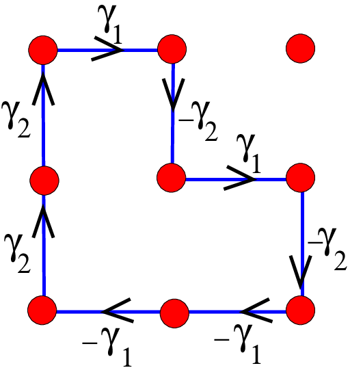
The basic idea of staggered fermions is to divide out this symmetry [157, 158, 159] by projecting out a single component of the fermion spinor on each site. Taking , one projector that accomplishes this is
| (12.387) |
where the are the integer coordinates of the respective lattice sites. This immediately reduces the doubling from a factor of sixteen to four. It is the various oscillating sign factors in this formula that give staggered fermions their name.
At this stage the naive axial symmetry remains. Indeed, the projector used above commutes with . This symmetry is allowed since four species, often called “tastes,” remain. Among them the symmetry is a taste non-singlet; under a chiral rotation, two rotate one way and two the other.
The next step taken by most of the groups using staggered fermions is the rooting trick. In the hope of reducing the multiplicity down from four, the determinant is replaced with its fourth root, . With several physical flavors this trick is applied separately to each. In simple perturbation theory this is correct since each fermion loop gets multiplied by one quarter, cancelling the extra factor from the four “tastes.”
At this point one should be extremely uneasy: the exact chiral symmetry is waving a huge red flag. Symmetries of the determinant survive rooting, and thus the exact axial symmetry for the massless theory remains. For the unrooted theory this was a flavored chiral symmetry. But, having reduced the theory to one flavor, how can there be a flavored symmetry without multiple flavors? We will now show why this rooting trick fails non-perturbatively when applied to the staggered quark operator.
12.5 The rooting issue
In previous sections we have seen that the chiral symmetry with fermion flavors has a rather complicated dependence on . With only one flavor there is no chiral symmetry at all, while in general if the fermions are massless, there are Goldstone bosons. We have also seen a qualitative difference in the mass dependence between an even and an odd number of species. Physics does not behave smoothly in the number of flavors and this raises issues for fermion formulations that inherently have multiple flavors, such as staggered fermions.
Starting with four flavors, the basic question is whether one can adjust down to one using the formal expression
| (12.388) |
This has been proposed and is widely used as a method for eliminating the extra species appearing with staggered fermion simulations.
At this point it is important to emphasize that asking about the viability of Eq. (12.388) is a vacuous question outside the context of a regulator. Field theory has divergences that need to be controlled, and, as we have seen above, the appearance of anomalies requires care. In particular, the regulated theory must explicitly break all anomalous symmetries in a way that survives in the continuum limit.
So we must apply Eq. (12.388) before removing the regulator. This is generally expected to be okay as long as the regulator breaks any anomalous symmetries appropriately on each of the four factors. For example, we expect rooting to be valid for four copies of the overlap operator. This satisfies a modified chiral symmetry where the gauge winding appears in the gauge dependent matrix through .
Section 10 showed that in the continuum with degenerate flavors there is a symmetry in mass parameter space corresponding to taking . Suppose we try to force the symmetry in the regulated theory before we root. This is easily accomplished by considering the determinant
| (12.389) |
This maintains the above symmetry through a permutation of the four flavors. This modification of the determinant still gives a valid formulation of the four flavor theory at vanishing because the imposed phases cancel. But expressed in this way, we start with four one-flavor theories each with a different value of . Were we to root this form, we would be averaging over four inequivalent theories. This is not expected to be correct, much as we would not expect rooting two different masses to give a theory of the average mass; i.e.
| (12.390) |
So we have presented both a correct and an incorrect way to root a four flavor theory down to one. What is the situation with staggered fermions, the primary place where rooting has been applied? The problem is that the kinetic term of the staggered action maintains one exact chiral symmetry even at finite lattice spacing. Without rooting this is flavor non-singlet amongst the “tastes.” As discussed earlier, there are two tastes of each chirality. But, because of this exact symmetry, which contains a subgroup, rooting to reduce the theory to one flavor is similar to the second case above and is not expected to be valid. In particular, rooting does not remove the discrete symmetry in the mass parameter, a symmetry which must not be present in the one flavor theory. Thus, just as in the above example, the tastes are not equivalent and rooting averages inequivalent theories.
The conclusion is that rooted staggered fermions are not QCD. So, what is expected to go wrong? The unbroken symmetry will give rise to extra minima in the effective potential as a function of and . In particular, for one flavor QCD one will get an effective potential with minima along the lines of Fig. 15 instead of the desired structure of Fig. 17. Forcing the extra minima would most likely drive the mass down from its physical value. This shift should be rather large, of order . This is testable, but being dominated by disconnected diagrams, may be rather difficult to verify in practice. In addition, if we vary the quark masses, the extra minima will result in phase transitions occurring whenever any single quark mass passes through zero. The previous discussion of the one flavor theory and the two flavor theory with non-degenerate quarks both show that this is unphysical; no structure is expected when only a single mass passes through zero.
This problem is admittedly subtle. Formula (12.388) seems
intuitively obvious and does work if the individual factors take care
of the possible anomalies, as with four copies of the overlap
operator. 1010
10
A few still hide behind this wall so frail,
So blind to chiral twists that made it fail.
It is also correct perturbatively, since the rooting factor
reduces any fermion loop by the correct amount. However, the basic
structure built up in earlier sections makes it indisputable that the
dependence of QCD on the parameter Theta is real. With the staggered
action, the distinct tastes are not equivalent due to their different
behavior under chiral rotations. It is this inequivalence that is at
the heart of the failure of rooting for this particular action.
Despite these problems, several lattice collaborations continue to pursue staggered fermions using the rooting trick [160, 161, 162]. The justification is partly because the simulations are slightly faster than using Wilson fermions, and partly because the exact chiral symmetry simplifies operator mixing. The success of a variety of calculations which are not strongly dependent on the anomaly shows the approach, while technically incorrect, is often a good approximation. On the other hand, if one’s goal is to test QCD as the theory of the strong interactions or to estimate QCD corrections to standard model processes [163], then one must be extremely wary of any discrepancies found using this method.
13 Other issues
13.1 Quantum fluctuations and topology
We have seen how zero modes of the Dirac operator are closely tied to the anomaly. And we have seen that for smooth classical fields, configurations that give zero modes for the classical Dirac operator do indeed exist. However, when getting into more detail with defining a lattice Dirac operator, we found subtle issues about which operator to use. And way back in Section 2 we saw that typical fields in path integrals are non-differentiable. This leads to the question of uniqueness for the winding number of a given gauge configuration. Indeed, is something like the topological susceptibility of the vacuum a true physical observable?
In [164] a definition of topological charge was constructed using the naive fermion operator as a regulator for the trace of as in the earlier derivation of the index theorem. This operator does not generally give an integer value for a typical gauge configuration in simulations. However, it does reduce to such after a cooling procedure is used to remove short distance fluctuations. The results of such are shown in Fig. 33. On the other hand, the gauge field space in lattice gauge theory is simply connected. Empirically with enough cooling, any gauge configuration appears to eventually decay to a state of zero action, gauge equivalent to the vacuum.

Since configurations appear to cool ultimately to trivial winding, using a cooling algorithm to define topology requires an arbitrary selection for cooling time. Modifying the Wilson action can prevent the winding decay. For example, forbidding the lattice action on any given plaquette from becoming larger than a small enough number can prevent instanton decay [165]. Such an “admissibility” condition, however, violates reflection positivity [98] and arbitrarily selects a special instanton size where the action is minimum.
Cooling time is not the only issue here. While attaining an integer winding requires cooling, note in Fig. 33 that the initial cooling stages seem quite chaotic. This raises the question of whether the discrete stages reached after some cooling might depend rather sensitively on the cooling algorithm. Figure 34 shows the evolution of a single lattice with three different relaxation algorithms. One algorithm consists of sweeping over the lattice using checkerboard ordering and replacing each link with the group element that minimizes the action associated with the given link. This is done by projecting the sum of staples that interact with the link onto the group. For the second approach, an under-relaxed algorithm adds the old link to the sum of the neighborhood staples before projecting onto the new group element. Finally, an over-relaxed approach subtracts the old element from the staple sum. The resulting windings not only depend on cooling time, but also on the specific algorithm chosen.

In an extensive analysis, Ref. [166] has compared a variety of filtering methods to expose topological structures in gauge configurations. All schemes have some ambiguities, but when the topological structures are clear, the various approaches when carefully tuned give similar results. Nevertheless the question remains of whether there is a rigorous and unambiguous definition of topology that applies to all typical configurations arising in a simulation. Luscher has discussed using a differential flow with the Wilson gauge action to accomplish the cooling [167]. This corresponds to the limit of maximal under-relaxation. This approach still allows the above topology collapse unless prevented by something like the admissibility condition or the selection of an arbitrary flow time. In addition, if one wishes to determine the topological charge of a configuration obtained in some large scale dynamical simulation, it is unclear why one should take the particular choice of the Wilson gauge action for the cooling procedure.
The high sensitivity to the cooling algorithm on rough gauge configurations suggests that there may be an inherent ambiguity in defining the topological charge of typical gauge configurations and consequently a small ambiguity in the definition of topological susceptibility. It also raises the question of how smooth is a given definition of topological charge as the gauge fields vary; how much correlation is there between nearby gauge configurations? Although such issues are quite old [168], they continue to be of considerable interest [169, 170, 171].
As topological charge is suppressed by light dynamical quarks, this is connected to the question discussed earlier of whether the concept of a single massless quark is well defined [31]. Dynamical quarks are expected to suppress topological structures, and the chiral limit with multiple massless quarks should give zero topological susceptibility with a chiral fermion operator, such as the overlap. However, with only a single light quark, the lack of chiral symmetry indicates that there is no physical singularity in the continuum theory as this mass passes through zero. Any scheme dependent ambiguity in defining the quark mass would then carry through to the topological susceptibility.
One might argue that the overlap operator solves this problem by defining the winding number as the number of zero eigenvalues of this quantity. Indeed, it has been shown [172, 171] that this definition gives a finite result in the continuum limit. As one is using the fermion operator only as a probe of the gluon fields, this definition can be reformulated directly in terms of the underlying Wilson operator [173]. While the result may have a finite continuum limit, the earlier discussion showed that the overlap operator is not unique. In particular it depends on the initial Dirac operator being projected onto the overlap circle. For the conventional Wilson kernel, there is a dependence on the parameter commonly referred to as the domain-wall height. Whether there is an ambiguity in the index defined this way depends on the density of real eigenvalues of the kernel in the vicinity of the point from which the projection is taken. Numerical evidence [148] suggests that this density decreases with lattice spacing, but it is unclear if this decrease is rapid enough to give a unique susceptibility in the continuum limit. The admissibility condition also successfully eliminates this ambiguity; however, as mentioned earlier, this condition is inconsistent with reflection positivity.
Whether topological susceptibility is well defined or not seems to have no particular phenomenological consequences. Indeed, this is not a quantity directly measured in any scattering experiment. It is only defined in the context of a technical definition in a particular non-perturbative simulation. Different valid schemes for regulating the theory might well come up with different values; it is only physical quantities such as hadronic masses that must match between approaches. The famous Witten-Veneziano relation [174, 175] does connect topological susceptibility of the pure gauge theory with the eta prime mass in the large number of colors limit. This mass, of course, remains well defined in the physical case of three colors, but the finite corrections to topology can depend delicately on gauge field fluctuations, which are the concern here.
13.2 The standard model
Throughout the above we have concentrated on the strong interactions. It is only for this sector of the standard model that perturbation theory fails so spectacularly. But the weak and electromagnetic interactions are crucial parts of the full standard model (gravitation is ignored here since it has even more serious unsolved problems). And for these interactions it is also true that the perturbative expansion does not converge. Because the underlying couplings are so small, this does not appear to be of any practical importance; however, conceptually it is quite desirable to have a lattice formulation for these interactions as well. From a purist point of view, the continuum limit of a lattice theory defines a continuum field theory. Thus without a lattice description of the other interactions it is unclear whether we can say they are well founded field theories.
In this context we note that the general picture of the standard model has changed dramatically over the years. Originally it was the successes of quantum electrodynamics that made it the model relativistic field theory. Before QCD, the strong interactions were a mystery. But now we see that because of asymptotic freedom, QCD on its own is likely to be a well defined and self contained theory. It is the electroweak theory, where both the electric charge and the Higgs couplings are not asymptotically free, for which we lack a non-perturbative formulation. Indeed, a speculative topic such as the possibility of emergent gravity may be intimately tied to these issues with the weaker forces.
For the electromagnetic interactions, a lattice formulation at first seems straightforward, involving the introduction of an additional gauge field for the photons. Unlike the strong interaction case, however, for electrodynamics we do not have asymptotic freedom to tell us how to take the continuum limit. And the physical coupling seems to be an unnaturally small number. Perhaps electrodynamics on its own does not actually exist as a field theory, much as believed for the scalar theory. But photons and electrons are essential components to the world around us. One interesting possibility is that electromagnetism is actually only a part of a higher level theory, perhaps in some unification with the strong interactions.
With the weak interactions we hit a more serious snag in that they are known to violate parity. The bosons appear to interact only with left handed fermions. As such we need to couple the fermions in a chiral manner, and it is not known how to do this in any non-perturbative scheme. The problem here is closely tied to the anomaly and the fact that not all currents can be simultaneously conserved. Indeed, when applied to the weak interactions, the ’t Hooft vertex gives rise to effective interactions that do not conserve baryon number. Any complete non-perturbative formulation must allow for such processes [176]. Some attempts to include such in a domain wall formulation have been presented [133, 177], but these generally involve heavy additional states such as “mirror” fermions [178]. While potentially viable, such approaches so far lack the theoretical elegance of the original Wilson lattice gauge theory. Indeed, it is the problem of chiral gauge theories that encourages studies of chiral symmetry from all possible angles.
Perhaps a lattice formulation more intimately tied to unification ideas could help here. The group looks quite interesting in this context [94]. Here a single generation of fermions fits nicely into a single 16 dimensional representation of this group. And in this picture anomalies are automatically cancelled. This would seem to indicate that there should be no obvious requirement for doublers as an obstacle to a lattice construction. However, the usual Wilson approach seems to require a term that is not a singlet under this group. This could be overcome with some added Higgs-like scalar fields, but then we get closer to the above mentioned models with the doublers playing the role of mirror fermions.
13.3 Where is the parity violation?
The standard model of elementary particle interactions is based on the product of three gauge groups, . Here the represents the strong interactions of quarks and gluons, the corresponds to electromagnetism, and the gives rise to the weak interactions. We ignore here the technical details of electroweak mixing. The full model is, of course, parity violating, as necessary to describe observed helicities in beta decay. This violation is normally considered to lie in the of the weak interactions, with both the and being parity conserving. We will show here that this is actually a convention, adopted primarily because the weak interactions are small compared to the others. We show below that reassigning degrees of freedom allows a reinterpretation where the gauge interaction is vector-like. Since the full model is parity violating, this process shifts the parity violation into the strong, electromagnetic, and Higgs interactions. The resulting theory pairs the left handed electron with a right handed anti-quark to form a Dirac fermion. With a vector-like weak interaction, the chiral issues which complicate lattice formulations now move to the other gauge groups. Requiring gauge invariance for the re-expressed electromagnetism then clarifies the mechanism behind one proposal for a lattice regularization of the standard model [179, 180].
For simplicity we consider here only the first generation, which involves four left handed doublets. These correspond to the neutrino/electron lepton pair plus three colors for the up/down quarks
| (13.391) |
Here the superscripts from the set represent the internal index of the strong interactions, and the subscript indicates left-handed helicities.
If we ignore the strong and electromagnetic interactions, leaving only the weak , each of these four doublets is equivalent and independent. We now arbitrarily pick two of them and do a charge conjugation operation, thus switching to their antiparticles
| (13.392) |
In four dimensions anti-fermions have the opposite helicity; so, we label these new doublets with representing right handedness.
With two left and two right handed doublets, we can combine them into two Dirac doublets
| (13.393) |
Formally in terms of the underlying fields, the construction takes
| (13.394) | |||
| (13.395) |
From the conventional point of view, these fields have rather peculiar quantum numbers. For example, the left and right parts have different electric charges. Electromagnetism now violates parity. The left and right parts also have different strong quantum numbers; the strong interactions violate parity as well. Finally, the components have different masses; parity is violated in the Higgs mechanism.
The different helicities of these fields also have variant baryon number. This is directly related to the known baryon violating processes through weak “instantons” and axial anomalies[21]. When a topologically non-trivial weak field is present, the axial anomaly arises from a level flow out of the Dirac sea [70]. This generates a spin flip in the fields, i.e. . Because of the peculiar particle identification, this process does not conserve charge, with . This would be a disaster for electromagnetism were it not for the fact that simultaneously the other Dirac doublet also flips with a compensating . This is anomaly cancellation, with the total . Only when both doublets are considered together is the symmetry restored. In this anomalous process baryon number is violated, with . This is the famous “ ‘t Hooft vertex” [21] discussed earlier in the context of the strong interactions.
13.4 A lattice model
The above discussion on twisting the gauge groups has been in the continuum. Now we turn to the lattice and show how this picture leads to a possible lattice model for the strong interactions, albeit with an unusual added coupling that renders the treatment quite difficult to make rigorous [179, 180]. Whether this model is viable remains undecided, but it does incorporate many of the required features.
For this we use the domain wall approach for the fermions [116, 134]. As discussed earlier, in this picture, our four dimensional world is a “4-brane” embedded in 5-dimensions. The complete lattice is a five dimensional box with open boundaries, and the parameters are chosen so the physical quarks and leptons appear as surface zero modes. The elegance of this scheme lies in the natural chirality of these modes as the size of the extra dimension grows. With a finite fifth dimension one doubling remains, coming from interfaces appearing as surface/anti-surface pairs. It is natural to couple a four dimensional gauge field equally to both surfaces, giving rise to a vector-like theory.
We now insert the above pairing into this five dimensional scheme. In particular, consider the left handed electron as a zero mode on one wall and the right handed anti-green-up-quark as the partner zero mode on the other wall, as sketched in Fig. 35. This provides a lattice regularization for the of the weak interactions.

However, since these two particles have different electric charge, must be broken in the interior of the extra dimension. We now proceed in analogy to the “waveguide” picture[181] and restrict this charge violation to to one layer at some interior position . Using Wilson fermions, the hopping term from to
| (13.396) |
is a operator. At this layer, electric charge is not conserved. This is unacceptable and needs to be fixed.
To restore the symmetry one must transfer the charge from to the compensating doublet . For this we replace the sum of hoppings with a product on the offending layer
| (13.397) |
This introduces an electrically neutral four-fermi operator. Note that it is baryon violating, involving a “lepto-quark/diquark” exchange, as sketched in Fig. 36. One might think of the operator as representing a “filter” at through which only charge compensating pairs of fermions can pass.

In five dimensions there is no chiral symmetry. Even for the free theory, combinations like have non-vanishing vacuum expectation values. We use such as a “tadpole,” with generating an effective hopping for and vice versa.
Actually the above four fermion operator is not quite sufficient for all chiral anomalies, which can also involve right handed singlet fermions. To correct this we need explicitly include the right handed sector, adding similar four fermion couplings (also electrically neutral). The main difference is that this sector does not couple to the weak bosons.
Having fixed the of electromagnetism, we restore the strong with an anti-symmetrization of the quark color indices in the new operator, . Note that similar left-right inter-sector couplings are needed to correctly obtain the effects of topologically non-trivial strong gauge fields.
An alternative view of this picture folds the lattice about the interior of the fifth dimension, placing all light modes on one wall and having the multi-fermion operator on the other. This is the model of Ref. [179], with the additional inter-sector couplings correcting a technical error [182].
Unfortunately the scheme is still not completely rigorous. In particular, the non-trivial four-fermion coupling represents a new defect and we need to show that this does not give rise to unwanted extra zero modes. Note, however, that the five dimensional mass is the same on both sides of defect; thus there are no topological reasons for such.
A second worry is that the four fermion coupling might induce an unwanted spontaneous symmetry breaking of one of the gauge symmetries. We need to remain in a strongly coupled paramagnetic phase without spontaneous symmetry breaking. Ref. [179] showed that strongly coupled zero modes do preserve the desired symmetries, but the analysis ignored contributions from heavy modes in the fifth dimension.
Assuming all works as desired, the model raises several other interesting questions. As formulated, we needed a right handed neutrino to provide all quarks with partners. Is there some variation that avoids this particle, which decouples from all gauge fields in the continuum limit? Another question concerns possible numerical simulations; is the effective action positive? Finally, we have used the details of the usual standard model, leaving open the question of whether this model is somehow special. Can we always find an appropriate multi-fermion coupling to eliminate undesired modes in other chiral theories where anomalies are properly canceled?
14 Final remarks
We have seen how many features of QCD are influenced by non-perturbative physics. This is particularly important to various aspects of chiral symmetry breaking. Taken as a whole, these fit together into a rather elegant and coherent picture. In particular, chiral symmetry is broken in three rather different ways. We have concentrated on the interplay of these mechanisms.
The primary and most important effect is the dynamical symmetry breaking that leads to the pions being light pseudo-Goldstone bosons. Their dynamics represents the most important physics for QCD at low energies. The popular and useful chiral expansion is a natural expansion in the momenta and masses of these particles.
In addition to the basic dynamical breaking is the anomaly, which eliminates the flavor-singlet axial symmetry of the classical theory. Thus the meson is not a Goldstone boson and acquires a mass of order . Understanding this breaking requires non-perturbative physics associated with the zero modes of the Dirac operator.
Finally, we have the explicit symmetry breaking from the quark masses. This is responsible for the pseudo-scalar mesons not being exactly massless. Using the freedom to redefine fields using chiral rotations, the number of independent mass parameters is where is the number fermion species under consideration. This includes the possibility of CP violation coming from the interplay of the mass term with the anomaly.
Throughout we have used only a few widely accepted assumptions, such as the existence of QCD as a field theory and standard ideas about chiral symmetry. Thus it is perhaps somewhat surprising that several of the conclusions remain controversial. The first of these is that chiral symmetry is lost in a theory with only one light quark. The resulting additive non-perturbative renormalization of the mass precludes using a massless up quark to solve the strong CP problem. Tied to this is the issue of whether topological susceptibility is well defined when non-differentiable fields dominate the path integral. Finally, probably the most bitter controversies revolve about the symmetries inherent in the staggered formulation and how these invalidate the use of rooting to remove unwanted degeneracies.
As simple as the overall picture is, it requires understanding effects that go well beyond perturbation theory. We need aspects of the Dirac spectrum that rely on gauge fields of non-trivial topology. Such appear already in the classical theory, although their true importance only appears in the context of the anomaly. Including this physics properly in a lattice formulation is a rich and sometimes controversial topic of active research.
The author is grateful to Ivan Horvath for suggesting this article. He is also indebted to Ivan as well as to Stefano Capitani and Nobuyoshi Ohta for finding numerous typos in the original version. The Alexander von Humboldt Foundation provided valuable support for visits to the University of Mainz where a portion of this research was carried out. This manuscript has been authored by employees of Brookhaven Science Associates, LLC under Contract No. DE-AC02-98CH10886 with the U.S. Department of Energy. The publisher by accepting the manuscript for publication acknowledges that the United States Government retains a non-exclusive, paid-up, irrevocable, world-wide license to publish or reproduce the published form of this manuscript, or allow others to do so, for United States Government purposes.
References
- [1] Murray Gell-Mann. A schematic model of baryons and mesons. Phys. Lett., 8:214–215, 1964.
- [2] Sanjib R. Mishra and Frank Sciulli. Deep inelastic lepton - nucleon scattering. Ann. Rev. Nucl. Part. Sci., 39:259–310, 1989.
- [3] P. D. B. Collins. An introduction to Regge theory and high-energy physics. Cambridge, 1977.
- [4] W. Meissner and R. Ochsenfeld. Ein neuer effekt bei eintritt der supraleitfähigkeit. Naturwissenschaften, 21:787–788, 1933.
- [5] A.A. Abrikosov. On the Magnetic properties of superconductors of the second group. Sov.Phys.JETP, 5:1174–1182, 1957.
- [6] H.F. Hess, R.B. Robinson, R.C. Dynes, J.M. Valles, and J.V. Waszczak. Scanning-Tunneling-Microscope Observation of the Abrikosov Flux Lattice and the Density of States near and inside a Fluxoid. Phys.Rev.Lett., 62:214–216, 1989.
- [7] A. Chodos, R. L. Jaffe, K. Johnson, Charles B. Thorn, and V. F. Weisskopf. A new extended model of hadrons. Phys. Rev., D9:3471–3495, 1974.
- [8] Chen-Ning Yang and Robert L. Mills. Conservation of Isotopic Spin and Isotopic Gauge Invariance. Phys.Rev., 96:191–195, 1954.
- [9] Kenneth G. Wilson. Confinement of quarks. Phys. Rev., D10:2445–2459, 1974.
- [10] Kenneth G. Wilson. Quarks and strings on a lattice. Erice Lectures 1975, 1977. New Phenomena In Subnuclear Physics. Part A. Proceedings of the First Half of the 1975 International School of Subnuclear Physics, Erice, Sicily, July 11 - August 1, 1975, ed. A. Zichichi, Plenum Press, New York, 1977, p. 69, CLNS-321.
- [11] F.J. Dyson. Divergence of perturbation theory in quantum electrodynamics. Phys.Rev., 85:631–632, 1952.
- [12] L.D. Landau and I.Ya. Pomeranchuk. On Point interactions in quantum electrodynamics. Dokl.Akad.Nauk Ser.Fiz., 102:489, 1955. Also published in Collected Papers of L.D. Landua. Edited by D. Ter Haar. Pergamon Press, 1965. pp. 654-658.
- [13] S. Mandelstam. Soliton Operators for the Quantized Sine-Gordon Equation. Phys.Rev., D11:3026, 1975.
- [14] Sidney R. Coleman. Classical Lumps and their Quantum Descendents. Subnucl.Ser., 13:297, 1977.
- [15] Julian S. Schwinger. Gauge Invariance and Mass. 2. Phys.Rev., 128:2425–2429, 1962.
- [16] Sidney R. Coleman. The Quantum Sine-Gordon Equation as the Massive Thirring Model. Phys.Rev., D11:2088, 1975.
- [17] Walter E. Thirring. A Soluble relativistic field theory? Annals Phys., 3:91–112, 1958.
- [18] C. Itzykson and J.M. Drouffe. Statistical field theory. Vol. 1: From Brownian motion to renormalization and lattice gauge theory. Cambridge, 1989.
- [19] Michael Creutz. Hidden symmetries in two dimensional field theory. Annals Phys., 321:2782–2792, 2006.
- [20] Roger F. Dashen. Some features of chiral symmetry breaking. Phys.Rev., D3:1879–1889, 1971.
- [21] Gerard ’t Hooft. Computation of the quantum effects due to a four-dimensional pseudoparticle. Phys.Rev., D14:3432–3450, 1976.
- [22] Edward Witten. Large N chiral dynamics. Annals Phys., 128:363, 1980.
- [23] C. Rosenzweig, J. Schechter, and C.G. Trahern. Is the effective lagrangian for QCD a Sigma model? Phys.Rev., D21:3388, 1980.
- [24] Richard L. Arnowitt and Pran Nath. Effective Lagrangians with U(1) axial anomaly. 1. Nucl.Phys., B209:234, 1982.
- [25] Pran Nath and Richard L. Arnowitt. Effective Lagrangians with axial anomaly. 2. Nucl.Phys., B209:251, 1982.
- [26] Ken Kawarabayashi and Nobuyoshi Ohta. The problem of eta in the large N limit: effective Lagrangian approach. Nucl.Phys., B175:477, 1980.
- [27] Ken Kawarabayashi and Nobuyoshi Ohta. On the partial conservation of the U(1) current. Prog.Theor.Phys., 66:1789, 1981.
- [28] Nobuyoshi Ohta. Vacuum structure and chiral charge quantization in the large N limit. Prog.Theor.Phys., 66:1408, 1981.
- [29] Daniel Boer and Jorn K. Boomsma. Spontaneous CP-violation in the strong interaction at theta = pi. Phys.Rev., D78:054027, 2008.
- [30] Michael Creutz. Quark masses and chiral symmetry. Phys. Rev., D52:2951–2959, 1995.
- [31] Michael Creutz. Ambiguities in the up quark mass. Phys. Rev. Lett., 92:162003, 2004.
- [32] Michael Creutz. Comments on staggered fermions / Panel discussion. PoS, CONFINEMENT8:016, 2008.
- [33] Tom Banks and A. Zaks. On the phase structure of vector-like gauge theories with massless fermions. Nucl.Phys., B196:189, 1982.
- [34] Michael Creutz. Gauge Fixing, the Transfer Matrix, and Confinement on a Lattice. Phys. Rev., D15:1128, 1977.
- [35] R.P. Feynman. Space-time approach to nonrelativistic quantum mechanics. Rev.Mod.Phys., 20:367–387, 1948.
- [36] Richard P. Feynman and A. R. Hibbs. Quantum mechanics and path integrals. McGraw Hill, 1965.
- [37] M. Creutz and B. Freedman. A statistical approach to quantum mechanics. Ann. Phys., 132:427, 1981.
- [38] Michael Creutz. Evaluating Grassmann integrals. Phys. Rev. Lett., 81:3555–3558, 1998.
- [39] Michael Creutz. Transfer matrices and lattice fermions at finite density. Found. Phys., 30:487–492, 2000.
- [40] M. Creutz. Quarks, gluons, and lattices. Cambridge, Uk: Univ. Pr. ( 1983) 169 P. ( Cambridge Monographs On Mathematical Physics).
- [41] Christof Gattringer and Christian B. Lang. Quantum chromodynamics on the lattice. Springer Lect.Notes Phys., 788:1–211, 2010.
- [42] I. Montvay and G. Munster. Quantum fields on a lattice. Cambridge, UK: Univ. Pr., 1994.
- [43] Thomas DeGrand and Carleton E. Detar. Lattice methods for quantum chromodynamics. World Scientific, 2006.
- [44] H.J. Rothe. Lattice gauge theories: an introduction. World Sci.Lect.Notes Phys., 74:1–605, 2005.
- [45] S. Elitzur. Impossibility of spontaneously breaking local symmetries. Phys.Rev., D12:3978–3982, 1975.
- [46] L.D. Faddeev and V.N. Popov. Feynman Diagrams for the Yang-Mills Field. Phys.Lett., B25:29–30, 1967.
- [47] I.M. Singer. Some remarks on the Gribov ambiguity. Commun.Math.Phys., 60:7–12, 1978.
- [48] M. Creutz. Monte Carlo Study of Quantized SU(2) Gauge Theory. Phys. Rev., D21:2308–2315, 1980.
- [49] Michael Creutz, Laurence Jacobs, and Claudio Rebbi. Monte Carlo Study of Abelian Lattice Gauge Theories. Phys. Rev., D20:1915, 1979.
- [50] N. Metropolis, A.W. Rosenbluth, M.N. Rosenbluth, A.H. Teller, and E. Teller. Equation of state calculations by fast computing machines. J.Chem.Phys., 21:1087–1092, 1953.
- [51] Neal Madras and Alan D. Sokal. The Pivot algorithm: a highly efficient Monte Carlo method for selfavoiding walk. J.Statist.Phys., 50:109–186, 1988.
- [52] D.H. Weingarten and D.N. Petcher. Monte Carlo integration for lattice gauge theories with fermions. Phys.Lett., B99:333, 1981.
- [53] F. Fucito, E. Marinari, G. Parisi, and C. Rebbi. A proposal for Monte Carlo simulations of fermionic Systems. Nucl.Phys., B180:369, 1981.
- [54] D.J. Scalapino and R.L. Sugar. A method for performing Monte Carlo calculations for systems with fermions. Phys.Rev.Lett., 46:519, 1981.
- [55] S. Duane, A.D. Kennedy, B.J. Pendleton, and D. Roweth. Hybrid Monte Carlo. Phys.Lett., B195:216–222, 1987.
- [56] M. Creutz. Global Monte Carlo algorithms for many-fermion systems. Phys. Rev., D38:1228–1238, 1988.
- [57] H.David Politzer. Reliable perturbative results for strong interactions? Phys.Rev.Lett., 30:1346–1349, 1973.
- [58] D.J. Gross and Frank Wilczek. Ultraviolet behavior of nonabelian gauge theories. Phys.Rev.Lett., 30:1343–1346, 1973.
- [59] D.J. Gross and Frank Wilczek. Asymptotically free gauge theories. 1. Phys.Rev., D8:3633–3652, 1973.
- [60] William E. Caswell. Asymptotic behavior of nonabelian gauge theories to two loop order. Phys.Rev.Lett., 33:244, 1974.
- [61] D.R.T. Jones. Two loop diagrams in Yang-Mills theory. Nucl.Phys., B75:531, 1974.
- [62] Sidney R. Coleman and Erick J. Weinberg. Radiative corrections as the origin of spontaneous symmetry breaking. Phys.Rev., D7:1888–1910, 1973.
- [63] J.A.M. Vermaseren, S.A. Larin, and T. van Ritbergen. The four loop quark mass anomalous dimension and the invariant quark mass. Phys.Lett., B405:327–333, 1997.
- [64] Konstantin G. Chetyrkin, Mikolaj Misiak, and Manfred Munz. Beta functions and anomalous dimensions up to three loops. Nucl.Phys., B518:473–494, 1998.
- [65] Anna Hasenfratz and Peter Hasenfratz. The connection between the Lambda parameters of lattice and continuum QCD. Phys.Lett., B93:165, 1980.
- [66] Anna Hasenfratz and Peter Hasenfratz. The scales of Euclidean and Hamiltonian lattice QCD. Nucl.Phys., B193:210, 1981.
- [67] Roger F. Dashen and David J. Gross. The relationship between lattice and continuum definitions of the gauge theory coupling. Phys.Rev., D23:2340, 1981.
- [68] K.G. Wilson and John B. Kogut. The Renormalization group and the epsilon expansion. Phys.Rept., 12:75–200, 1974.
- [69] R. Rajaraman. Solitons and instantons. An introduction to solitons and instantons in quantum field theory. North-holland, 1982.
- [70] Jan Ambjorn, J. Greensite, and C. Peterson. The axial anomaly and the lattice dirac sea. Nucl.Phys., B221:381, 1983.
- [71] Ettore Vicari and Haralambos Panagopoulos. Theta dependence of gauge theories in the presence of a topological term. Phys.Rept., 470:93–150, 2009.
- [72] Jeffrey Goldstone, Abdus Salam, and Steven Weinberg. Broken Symmetries. Phys.Rev., 127:965–970, 1962.
- [73] Julian S. Schwinger. Field theory commutators. Phys.Rev.Lett., 3:296–297, 1959.
- [74] Michael Creutz. Anomalies and chiral symmetry in QCD. Annals Phys., 324:1573–1584, 2009.
- [75] J. D. Bjorken. Inequality for backward electron-nucleon and muon-nucleon scattering at high momentum transfer. Phys. Rev., 163:1767–1769, 1967.
- [76] J. D. Bjorken. Applications of the chiral algebra of current densities. Phys. Rev., 148:1467–1478, 1966.
- [77] David B. Kaplan and Aneesh V. Manohar. Current Mass Ratios of the Light Quarks. Phys.Rev.Lett., 56:2004, 1986.
- [78] Steven Weinberg. The Problem of Mass. Trans.New York Acad.Sci., 38:185–201, 1977.
- [79] H. Leutwyler. The Ratios of the light quark masses. Phys.Lett., B378:313–318, 1996.
- [80] Michael Creutz. Spontaneous violation of CP symmetry in the strong interactions. Phys. Rev. Lett., 92:201601, 2004.
- [81] Stephen L. Adler. Axial vector vertex in spinor electrodynamics. Phys.Rev., 177:2426–2438, 1969.
- [82] Stephen L. Adler and William A. Bardeen. Absence of higher order corrections in the anomalous axial vector divergence equation. Phys.Rev., 182:1517–1536, 1969.
- [83] J.S. Bell and R. Jackiw. A PCAC puzzle: pi0 to gamma gamma in the sigma model. Nuovo Cim., A60:47–61, 1969.
- [84] Kazuo Fujikawa. Path integral measure for gauge invariant fermion theories. Phys.Rev.Lett., 42:1195, 1979.
- [85] Sidney R. Coleman. The uses of instantons. Subnucl.Ser., 15:805, 1979.
- [86] Paul H. Ginsparg and Kenneth G. Wilson. A remnant of chiral symmetry on the lattice. Phys.Rev., D25:2649, 1982.
- [87] Herbert Neuberger. Exactly massless quarks on the lattice. Phys.Lett., B417:141–144, 1998.
- [88] Tom Banks and A. Casher. Chiral symmetry breaking in confining theories. Nucl.Phys., B169:103, 1980.
- [89] Edward Witten. Constraints on supersymmetry breaking. Nucl.Phys., B202:253, 1982.
- [90] Edward Corrigan and Pierre Ramond. A note on the quark content of large color groups. Phys.Lett., B87:73, 1979.
- [91] A. Armoni, M. Shifman, and G. Veneziano. SUSY relics in one flavor QCD from a new 1/N expansion. Phys.Rev.Lett., 91:191601, 2003.
- [92] F. Sannino and M. Shifman. Effective Lagrangians for orientifold theories. Phys.Rev., D69:125004, 2004.
- [93] Mithat Unsal and Laurence G. Yaffe. (In)validity of large N orientifold equivalence. Phys.Rev., D74:105019, 2006.
- [94] Howard Georgi and Dimitri V. Nanopoulos. Ordinary predictions from grand principles: T quark mass in O(10). Nucl.Phys., B155:52, 1979.
- [95] Cumrun Vafa and Edward Witten. Parity conservation in QCD. Phys.Rev.Lett., 53:535, 1984.
- [96] Michael Creutz. One flavor QCD. Annals Phys., 322:1518–1540, 2007.
- [97] Michael Creutz. The ’t Hooft vertex revisited. Annals Phys., 323:2349–2365, 2008.
- [98] Michael Creutz. Positivity and topology in lattice gauge theory. Phys. Rev., D70:091501, 2004.
- [99] Michael Creutz. Quark mass dependence of two-flavor QCD. Phys. Rev., D83:016005, 2011.
- [100] Howard Georgi and Ian N. McArthur. Instantons and the Quark Mass. unpublished (HUTP-81/A011), 1981.
- [101] Tom Banks, Yosef Nir, and Nathan Seiberg. Missing (up) mass, accidental anomalous symmetries, and the strong CP problem. unpublished (hep-ph/9403203), 1994.
- [102] Michael Creutz. CP symmetry and the strong interactions. unpublished (hep-th/0303254), 2003.
- [103] Roberto Frezzotti, Pietro Antonio Grassi, Stefan Sint, and Peter Weisz. Lattice QCD with a chirally twisted mass term. JHEP, 0108:058, 2001.
- [104] Ph. Boucaud et al. Dynamical twisted mass fermions with light quarks. Phys.Lett., B650:304–311, 2007.
- [105] Varouzhan Baluni. CP Violating Effects in QCD. Phys.Rev., D19:2227–2230, 1979.
- [106] Michael Creutz. Isospin breaking and the chiral condensate. PoS, LAT2005:119, 2006.
- [107] Sinya Aoki. New Phase Structure for Lattice QCD with Wilson fermions. Phys.Rev., D30:2653, 1984.
- [108] Holger Bech Nielsen and M. Ninomiya. Absence of neutrinos on a lattice. 1. proof by homotopy theory. Nucl.Phys., B185:20, 1981.
- [109] Michael Creutz. Effective potentials, thermodynamics, and twisted mass quarks. Phys. Rev., D76:054501, 2007.
- [110] Michael Creutz. Wilson fermions at finite temperature. 1996. RHIC Summer Study ’96: Theory workshop on relativistic heavy ion collisions, D. Kahana and Y. Pang, eds., pp. 49-54 (NTIS, 1997); hep-lat/9608024.
- [111] Stephen R. Sharpe and Jr Singleton, Robert L. Spontaneous flavor and parity breaking with Wilson fermions. Phys.Rev., D58:074501, 1998.
- [112] P.H. Damgaard, K. Splittorff, and J.J.M. Verbaarschot. Microscopic Spectrum of the Wilson Dirac Operator. Phys.Rev.Lett., 105:162002, 2010.
- [113] R. Frezzotti and G.C. Rossi. Chirally improving Wilson fermions. 1. O(a) improvement. JHEP, 0408:007, 2004.
- [114] Gernot Munster, Christian Schmidt, and Enno E. Scholz. Chiral perturbation theory for twisted mass QCD. Nucl.Phys.Proc.Suppl., 140:320–322, 2005.
- [115] Rajamani Narayanan and Herbert Neuberger. A Construction of lattice chiral gauge theories. Nucl.Phys., B443:305–385, 1995.
- [116] David B. Kaplan. A method for simulating chiral fermions on the lattice. Phys. Lett., B288:342–347, 1992.
- [117] Vadim Furman and Yigal Shamir. Axial symmetries in lattice QCD with Kaplan fermions. Nucl.Phys., B439:54–78, 1995.
- [118] Michael Creutz. The evil that is rooting. Phys. Lett., B649:230–234, 2007.
- [119] Michael Creutz. Four-dimensional graphene and chiral fermions. JHEP, 04:017, 2008.
- [120] Tatsuhiro Misumi, Michael Creutz, and Taro Kimura. Classification and Generalization of Minimal-doubling actions. PoS, LATTICE2010:260, 2010.
- [121] Luuk H. Karsten. Lattice fermions in euclidean space-time. Phys.Lett., B104:315, 1981.
- [122] Frank Wilczek. On lattice fermions. Phys.Rev.Lett., 59:2397, 1987.
- [123] Artan Borici. Creutz fermions on an orthogonal lattice. Phys.Rev., D78:074504, 2008.
- [124] Paulo F. Bedaque, Michael I. Buchoff, Brian C. Tiburzi, and Andre Walker-Loud. Search for fermion actions on hyperdiamond lattices. Phys.Rev., D78:017502, 2008.
- [125] Taro Kimura and Tatsuhiro Misumi. Lattice fermions based on higher-dimensional hyperdiamond lattices. Prog.Theor.Phys., 123:63–78, 2010.
- [126] Michael Creutz and Tatsuhiro Misumi. Classification of Minimally Doubled Fermions. Phys. Rev., D82:074502, 2010.
- [127] Michael Creutz. Why rooting fails. PoS, LAT2007:007, 2007.
- [128] Michael Creutz. Anomalies and discrete chiral symmetries. PoS, QCD-TNT09:008, 2009.
- [129] Stefano Capitani, Michael Creutz, Johannes Weber, and Hartmut Wittig. Renormalization of minimally doubled fermions. JHEP, 09:027, 2010.
- [130] Brian C. Tiburzi. Chiral lattice fermions, minimal doubling, and the axial anomaly. Phys.Rev., D82:034511, 2010.
- [131] Rajamani Narayanan and Herbert Neuberger. Chiral determinant as an overlap of two vacua. Nucl. Phys., B412:574–606, 1994.
- [132] Karl Jansen. Domain wall fermions and chiral gauge theories. Phys. Rept., 273:1–54, 1996.
- [133] Michael Creutz and Ivan Horvath. Surface states and chiral symmetry on the lattice. Phys. Rev., D50:2297–2308, 1994.
- [134] Yigal Shamir. Chiral fermions from lattice boundaries. Nucl. Phys., B406:90–106, 1993.
- [135] Rajamani Narayanan and Herbert Neuberger. Infinitely many regulator fields for chiral fermions. Phys. Lett., B302:62–69, 1993.
- [136] Herbert Neuberger. A practical implementation of the overlap Dirac operator. Phys.Rev.Lett., 81:4060–4062, 1998.
- [137] Herbert Neuberger. More about exactly massless quarks on the lattice. Phys.Lett., B427:353–355, 1998.
- [138] Ting-Wai Chiu and Sergei V. Zenkin. On solutions of the Ginsparg-Wilson relation. Phys.Rev., D59:074501, 1999.
- [139] Shailesh Chandrasekharan. Lattice QCD with Ginsparg-Wilson fermions. Phys.Rev., D60:074503, 1999.
- [140] Peter Hasenfratz, Victor Laliena, and Ferenc Niedermayer. The index theorem in QCD with a finite cutoff. Phys.Lett., B427:125–131, 1998.
- [141] Peter Hasenfratz. Lattice QCD without tuning, mixing and current renormalization. Nucl.Phys., B525:401–409, 1998.
- [142] Michael Creutz. Transiting topological sectors with the overlap. Nucl. Phys. Proc. Suppl., 119:837–839, 2003.
- [143] Martin Luscher. Exact chiral symmetry on the lattice and the Ginsparg-Wilson relation. Phys.Lett., B428:342–345, 1998.
- [144] H. Neuberger. Overlap. Chin.J.Phys., 38:533–542, 2000.
- [145] Pilar Hernandez, Karl Jansen, and Martin Luscher. Locality properties of Neuberger’s lattice Dirac operator. Nucl.Phys., B552:363–378, 1999.
- [146] Ivan Horvath. Ginsparg-Wilson relation and ultralocality. Phys.Rev.Lett., 81:4063–4066, 1998.
- [147] Ivan Horvath. Ginsparg-Wilson-Luscher symmetry and ultralocality. Phys.Rev., D60:034510, 1999.
- [148] Robert G. Edwards, Urs M. Heller, and Rajamani Narayanan. A study of chiral symmetry in quenched QCD using the overlap Dirac operator. Phys.Rev., D59:094510, 1999.
- [149] Artan Borici. Lanczos approach to the inverse square root of a large and sparse matrix. J.Comput.Phys., 162:123–131, 2000.
- [150] S.J. Dong, F.X. Lee, K.F. Liu, and J.B. Zhang. Chiral symmetry, quark mass, and scaling of the overlap fermions. Phys.Rev.Lett., 85:5051–5054, 2000.
- [151] Christof Gattringer. A New approach to Ginsparg-Wilson fermions. Phys.Rev., D63:114501, 2001.
- [152] Martin Luscher. Lattice regularization of chiral gauge theories to all orders of perturbation theory. JHEP, 0006:028, 2000.
- [153] Yoshio Kikukawa and Atsushi Yamada. Weak coupling expansion of massless QCD with a Ginsparg-Wilson fermion and axial U(1) anomaly. Phys.Lett., B448:265–274, 1999.
- [154] Gerard ’t Hooft. Naturalness, chiral symmetry, and spontaneous chiral symmetry breaking. NATO Adv.Study Inst.Ser.B Phys., 59:135, 1980.
- [155] Robert G. Edwards, Urs M. Heller, and Rajamani Narayanan. Evidence for fractional topological charge in SU(2) pure Yang-Mills theory. Phys.Lett., B438:96–98, 1998.
- [156] Luuk H. Karsten and Jan Smit. Lattice fermions: species doubling, chiral invariance, and the triangle anomaly. Nucl.Phys., B183:103, 1981.
- [157] John B. Kogut and Leonard Susskind. Hamiltonian formulation of Wilson’s lattice gauge theories. Phys.Rev., D11:395, 1975.
- [158] Leonard Susskind. Lattice fermions. Phys.Rev., D16:3031–3039, 1977.
- [159] H.S. Sharatchandra, H.J. Thun, and P. Weisz. Susskind fermions on a Euclidean lattice. Nucl.Phys., B192:205, 1981.
- [160] Y. Aoki, Z. Fodor, S.D. Katz, and K.K. Szabo. The QCD transition temperature: Results with physical masses in the continuum limit. Phys.Lett., B643:46–54, 2006.
- [161] M. Cheng, N.H. Christ, S. Datta, J. van der Heide, C. Jung, et al. The QCD equation of state with almost physical quark masses. Phys.Rev., D77:014511, 2008.
- [162] A. Bazavov, D. Toussaint, C. Bernard, J. Laiho, C. DeTar, et al. Nonperturbative QCD simulations with 2+1 flavors of improved staggered quarks. Rev.Mod.Phys., 82:1349–1417, 2010.
- [163] E. Lunghi and Amarjit Soni. Possible evidence for the breakdown of the CKM-paradigm of CP-violation. Phys.Lett., B697:323–328, 2011.
- [164] Michael Creutz. Anomalies, gauge field topology, and the lattice. Annals Phys., 326:911–925, 2011.
- [165] M. Luscher. Topology of Lattice Gauge Fields. Commun.Math.Phys., 85:39, 1982.
- [166] Falk Bruckmann, Christof Gattringer, Ernst-Michael Ilgenfritz, Michael Muller-Preussker, Andreas Schafer, et al. Quantitative comparison of filtering methods in lattice QCD. Eur.Phys.J., A33:333–338, 2007.
- [167] Martin Luscher. Properties and uses of the Wilson flow in lattice QCD. JHEP, 1008:071, 2010.
- [168] M. Teper. Instantons in the quantized su(2) vacuum: A lattice monte carlo investigation. Phys.Lett., B162:357, 1985.
- [169] Falk Bruckmann, Florian Gruber, Karl Jansen, Marina Marinkovic, Carsten Urbach, et al. Comparing topological charge definitions using topology fixing actions. Eur.Phys.J., A43:303–311, 2010.
- [170] Peter J. Moran, Derek B. Leinweber, and Jianbo Zhang. Wilson mass dependence of the overlap topological charge density. 2010.
- [171] Martin Luscher. Topological effects in QCD and the problem of short distance singularities. Phys.Lett., B593:296–301, 2004.
- [172] Leonardo Giusti, G.C. Rossi, and M. Testa. Topological susceptibility in full QCD with Ginsparg-Wilson fermions. Phys.Lett., B587:157–166, 2004.
- [173] Martin Luscher and Filippo Palombi. Universality of the topological susceptibility in the SU(3) gauge theory. JHEP, 1009:110, 2010.
- [174] Edward Witten. Current algebra theorems for the goldstone boson. Nucl.Phys., B156:269, 1979.
- [175] G. Veneziano. without instantons. Nucl.Phys., B159:213–224, 1979.
- [176] Estia Eichten and John Preskill. Chiral gauge theories on the lattice. Nucl. Phys., B268:179, 1986.
- [177] Erich Poppitz and Yanwen Shang. Chiral lattice gauge theories via mirror-fermion decoupling: a mission (im)possible? Int.J.Mod.Phys., A25:2761–2813, 2010.
- [178] I. Montvay. A chiral SU(2)-L x SU(2)-R gauge model on the lattice. Phys. Lett., B199:89, 1987.
- [179] Michael Creutz, Michel Tytgat, Claudio Rebbi, and She-Sheng Xue. Lattice formulation of the standard model. Phys. Lett., B402:341–345, 1997.
- [180] Michael Creutz. Is the doubler of the electron an antiquark? Nucl. Phys. Proc. Suppl., 63:599–601, 1998.
- [181] Maarten F.L. Golterman, Karl Jansen, Donald N. Petcher, and Jeroen C. Vink. Investigation of the domain wall fermion approach to chiral gauge theories on the lattice. Phys.Rev., D49:1606–1620, 1994.
- [182] Herbert Neuberger. Comments on ’Lattice formulation of the standard model’ by Creutz, et al. Phys.Lett., B413:387–390, 1997.