The Conformal Sector of F-theory GUTs
Abstract
D3-brane probes of exceptional Yukawa points in F-theory GUTs are natural hidden sectors for particle phenomenology. We find that coupling the probe to the MSSM yields a new class of conformal fixed points with computable infrared R-charges. Quite surprisingly, we find that the MSSM only weakly mixes with the strongly coupled sector in the sense that the MSSM fields pick up small exactly computable anomalous dimensions. Additionally, we find that although the states of the probe sector transform as complete GUT multiplets, their coupling to Standard Model fields leads to a calculable threshold correction to the running of the visible sector gauge couplings which improves precision unification. We also briefly consider scenarios in which SUSY is broken in the hidden sector. This leads to a gauge mediated spectrum for the gauginos and first two superpartner generations, with additional contributions to the third generation superpartners and Higgs sector.
1 Introduction
F-theory provides a promising starting point for connecting string theory with particle phenomenology. In particular, Grand Unified Theories (GUTs) can be elegantly realized in this setup [1, 2, 3, 4] (see [5, 6] for reviews). Such scenarios feature higher dimensional GUT theories where the GUT group is localized on a seven-brane, and matter is trapped at the intersection of the GUT brane with additional flavor seven-branes. Interactions are localized at common intersections of the matter fields. The F-theory approach to particle physics is promising because while it is flexible enough to accommodate the basic features of realistic particle phenomenology, it is also rigid enough to impose non-trivial constraints on potential scenarios of physics beyond the Standard Model (SM).
One example of a such a constraint is that generating a large top quark mass requires the existence of exceptional (e.g. E-type) symmetry enhancement points in the geometry [1, 3]. Another example is that in geometrically minimal realizations of flavor hierarchies, both the CKM matrix and the mass matrices are in relatively close accord with observation [7, 8, 9, 10]. Certain supersymmetry (SUSY) breaking scenarios such as a “PQ deformation” of minimal gauge mediation can also be accommodated [11] in which the messenger fields localize on curves of the geometry. Combining this with other geometric conditions imposes constraints missing from purely low energy considerations; for example, in many models the representation content of the messengers is fixed by the available ways to unfold a singularity [12]. This is quite economical and constitutes a self-contained package. Nevertheless, given the existence of an entire landscape of possible closed string vacua, it is important to investigate possible well-motivated extensions of this framework.
A robust feature of this setup is that the possible ways to extend such GUT models by additional seven-brane intersections are rather limited. Aside from seven-branes, the main ingredients generically present in compactifications of F-theory are probe D3-branes. Such D3-branes fill 3+1 noncompact spacetime dimensions and sit at points of the internal geometry. Their presence in a globally complete compactification is often required in order to cancel tadpoles. Moreover, they are also locally attracted to the E-type Yukawa points of the visible sector [13]. It is therefore natural to ask what type of extra sectors are realized on such probe theories. At a generic internal point of the geometry, this extra sector is not terribly interesting. For example, a single D3-brane realizes Super Yang-Mills theory. In this theory, the vevs of the three chiral fields control the local position of the D3-brane in the three complex-dimensional internal geometry.
However, there is a distinguished point in F-theory phenomenology where intersecting seven-branes realize an exceptional symmetry. In geometrically minimal constructions, a single point of is responsible for generating all of the relevant visible sector Yukawa couplings [10, 12]. Since the D3-brane is attracted to such Yukawa points (see [14, 9, 13]), it is natural to ask what happens if D3-branes reside at (or very near) such a point. It was with this motivation in mind that these theories were proposed as possible quasi-hidden sectors for F-theory GUTs in [13] which were further studied in [15, 16].
The dominant couplings between the probe and Standard Model (SM) degrees of freedom have been studied in [13, 17]. Some of the states of the probe are charged under and therefore communicate via gauge interactions with the visible sector. Another source of probe/MSSM couplings is via F-terms. These F-terms primarily couple the probe to the Higgs fields and third generation of matter fields. This is because in the flavor hierarchy scenario of [7, 10, 12], these are the modes with maximum overlap with the Yukawa point, which is also the location of the D3-brane.
In the limit where one neglects the effects of the Standard Model fields, it was found in [15] that such probe theories realize a new class of strongly interacting superconformal field theories (SCFTs). These theories are defined by starting from the Minahan-Nemeschansky theories with flavor symmetry [18, 19], and adding a set of field-dependent mass deformations in the factor of . The choice of mass deformations is dictated by the local configuration of intersecting seven-branes. Remarkably, the configurations which lead to new fixed points are precisely those which are of most relevance for phenomenology.
With an eye towards potential model building applications, in this paper we take the next step in this analysis by coupling the probe to a dynamical visible sector. In other words, at the GUT scale , we consider performing a further deformation of the theories studied in [15]. This deformation induces a flow to another class of interacting CFTs. Much as in [15], we can compute various details of the system such as the scaling dimension of chiral operators, as well as the running of the visible sector gauge couplings. Although the combined probe/MSSM system realizes an interacting conformal fixed point, there is a well-defined sense in which the mixing between the two sectors remains small. Indeed, we find that the scaling dimensions of the SM chiral fields remains rather close to their free field values, with anomalous dimensions typically in the range of .
Since the CFT living on the D3-brane includes degrees of freedom charged under , these modes must develop a mass to have evaded detection thus far. This places a lower bound on the CFT breaking scale of order TeV. It is natural to ask how to break conformal invariance. A simple possibility is to have the D3-brane slightly displaced from the Yukawa point, since the displacement automatically introduces a scale and gives mass to these charged states of the probe sector.
Treating the SM gauge group as a weakly gauged flavor symmetry of the conformal fixed point, we calculate the contribution of the probe to the running of the SM gauge couplings. Introducing a characteristic scale associated with conformal symmetry breaking, we can view this computation as a threshold correction to the running of the MSSM gauge couplings which enters at energies . We find that although the states of the probe sector fill out full GUT multiplets, the additional charged degrees of freedom of the CFT improve precision unification of the MSSM (which for typical superpartner masses otherwise contains an order mismatch at two loop level) due to their breaking couplings to the Higgs sector (see also [20]). See figure 1 for a depiction of these effects.

It is also natural to ask what effect the D3-brane has on the visible sector at energies below . At this point there are two possibilities, depending on whether or not SUSY breaking takes place on the D3-brane hidden sector. If it does not, the story is rather simple, and the only remaining effects may include some light remnants which interact via kinetic mixing with the visible sector [13, 16].
If, however, SUSY breaking takes place on the D3-brane, the pattern of soft supersymmetry breaking terms in the visible sector may be strongly affected. Along these lines, the most natural thing to assume is that the D3-brane position mode which breaks conformal invariance also develops a SUSY breaking vev. Assuming this, the charged mediator states from the probe to the visible sector play the role of messenger fields in a minimal gauge mediation scenario, leading to a very predictive superpartner mass spectrum. The dominant coupling to the third generation and Higgs fields induces further corrections to the gauge mediated spectrum. These additional contributions can induce additional third generation/Higgs sector soft masses and large -terms, as well as and -terms.
The organization of this paper is as follows. In section 2 we review the basic features of the visible sector in F-theory GUTs, and the precise definition of the probe sectors we study in the remainder of this paper. In section 3 we study the infrared fixed points associated with coupling the MSSM to the probe. Using these results, in section 4 we demonstrate that for appropriate threshold scales, the presence of the probe can actually improve precision unification. We next turn in section 5 to the potential role of the probe as a sector for supersymmetry breaking and transmission to the visible sector. Section 6 contains our conclusions. A brief review of probes of T-Branes is given in Appendix A, and a collection of additional monodromy scenarios is collected in Appendix B.
2 Quasi-Hidden Sectors From F-theory
In this section we review the basic setup we shall be considering. The main idea is that the Standard Model is realized via a configuration of intersecting seven-branes in F-theory, and that D3-branes constitute an additional sector which can interact non-trivially with this system. Throughout, we shall work in terms of a limit where four-dimensional gravity has been decoupled, so that . This approximation is especially well-justified in systems where we focus on just the local intersections of non-compact seven-branes probed by a D3-brane which is pointlike in the internal directions. We now turn to a more precise characterization of the system we shall study.
2.1 Intersecting Seven-Branes and the Visible Sector
F-theory is a non-perturbative formulation of IIB string theory in which the axio-dilaton can attain order one values, which moreover can have non-trivial position dependence on the internal directions. Going to strong coupling provides a way to realize intersecting brane configurations with E-type symmetries. E-type symmetries are quite important in string-based GUT models, thus suggesting F-theory GUTs as a natural framework for string model building [1, 2, 3, 4]. The profile of the dilaton is, in minimal Weierstrass form, dictated by the equation:
| (2.1) |
Here, , and define three local complex coordinates for the threefold base of any F-theory compactification. The modular parameter of this elliptic curve is the axio-dilaton . The location of the intersecting seven-branes is then given by the discriminant
| (2.2) |
In such models, the visible sector is realized on a configuration of interecting seven-branes. The local intersections of such seven-branes can be modelled in terms of eight-dimensional Super Yang-Mills theory with gauge group . We denote by and two local complex coordinates parameterizing the internal worldvolume of the parent theory. The breaking pattern of then dictates the locations of localized matter, as well as the interactions between this matter [21, 1, 22, 17]. For the purposes of GUT model building, it is most convenient to work in terms of gauge theory. The particular choice of a breaking pattern in a local patch of the geometry is dictated by an adjoint-valued form which we denote by . This , along with the internal gauge fields of the seven-branes, satisfy a coupled system of F- and D-term equations. For example, to realize an F-theory GUT, one considers the breaking pattern:
| (2.3) |
where takes values in the adjoint of . This tilting of the seven-brane configuration occurs at an energy scale which we shall refer to as . The compactification of the seven-brane is assumed to occur at the GUT scale . Numerically, we have GeV and GeV [2].
The particular choice of dictates the phenomenology of the visible sector. A very convenient way to analyze supersymmetric configurations of intersecting seven-branes is in terms of “holomorphic gauge.” This choice amounts to analyzing just the F-term equations of motion for the system, and effectively complexifying the gauge group to . In an appropriate gauge, one can then locally present as a purely holomorphic expression in the local coordinates , of the parent theory worldvolume coordinates. In realistic F-theory GUT configurations, the actual seven-brane configuration corresponds to a “T-brane” [17]. Locally, this configuration is specified by the condition that at the origin, is nilpotent but non-zero. In holomorphic gauge, can then be decomposed into a direct sum of nilpotent Jordan blocks.
2.2 Review of Probe D3-Branes
So far, our discussion has focussed on the properties of the visible sector, e.g., the seven-branes of the system. An additional well-motivated sector to consider is one with D3-brane probes of such intersecting brane configurations. Away from the configuration of seven-brane intersections, the probe D3-brane is given by Super Yang-Mills theory with gauge group. The worldvolume gauge coupling is the IIB axio-dilaton . As the D3-brane moves closer to the configuration of intersecting seven-branes, additional modes will become light. This can lead to highly non-trivial interacting superconformal field theories.
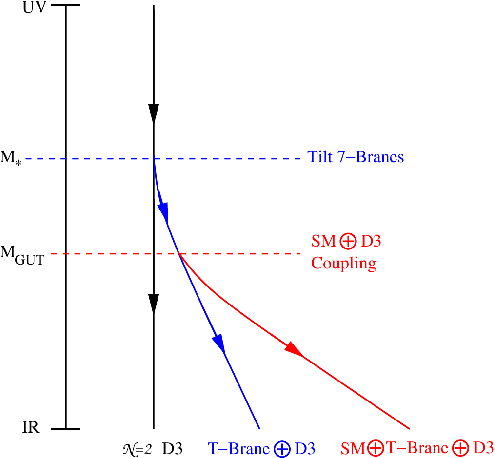
It is helpful to organize our discussion according to the energy scales of the probe system. See figure 2 for a depiction of the various energy scales and corresponding deformations of the probe/MSSM system. At high energies, when the seven-brane configuration is parallel, the probe realizes an theory. The effects of seven-brane tilting are then reflected in the probe theory as a combination of F- and D-term deformations, which are added at the scale . A further deformation appears at the GUT scale, because this is the scale at which the fields of the Standard Model become dynamical modes of the four-dimensional theory. One of the aims of this paper is to show that in the absence of other effects, these deformations lead to interacting fixed points for the combined probe/MSSM system.
Throughout this work, we will have occasion to refer to the various string states connecting the seven-branes and three-branes. We label the visible sector stack as a -brane, and the “flavor brane” as a -brane. The states in the worldvolume theory of the three-brane probe will come from the various types of or strings. We refer to states of the probe sector which are also charged under the SM gauge group as strings, and those strings which are neutral under as strings. There are also various types of strings as well, which are important for realizing the visible sector. Let us note that this is a slight abuse of terminology, because the actual modes will involve both weakly coupled strings, as well as strings and their junctions [23, 24, 25, 26].
The examples which have been most extensively studied in the literature correspond to worldvolume theories which retain supersymmetry. In this case, there is a single stack of parallel seven-branes with gauge group . This becomes a flavor symmetry of the probe theory. A remarkable feature of these probe theories is that the associated Seiberg-Witten curve is given by the same F-theory geometry [27, 28]. Examples of such probe theories include SYM with four flavors [28], Argyres-Douglas fixed points [29], and the Minahan-Nemeschansky theories with exceptional flavor symmetry [18, 19]. Although the first example is simply a D3-brane probing a seven-brane, the latter two possibilities are realized by D3-branes probing F-theory singularities of type and , and these involve intrinsically non-perturbative ingredients. This means that such theories are strongly coupled. The moduli space of the single D3-brane probe theory is given by a Higgs branch and a Coulomb branch. These are, respectively, parameterized by the vev of a dimension two operator in the adjoint of the flavor group , and the vev of a field which parameterizes motion normal to the seven-brane. In addition, there is a decoupled hypermultiplet parameterizing motion parallel to the seven-brane.
In the weakly coupled example given by a D3-brane probing a singularity, we have super Yang-Mills theory with gauge group and hypermultiplets . In this case, the operator is given by and has scaling dimension two. In a theory with exceptional flavor symmetries we lose any description of this operator in terms of elementary fields, although one can show there are still dimension two operators parameterizing the Higgs branch.
Tilting the seven-branes at a scale corresponds in the D3-brane theory to coupling the position modes and to the theory. This coupling breaks breaks part of the flavor symmetry. Although we find the breaking to be most useful for model building purposes, there is no a priori reason that we could not choose a different breaking pattern. This tilting gives a mass to some of the strings, and is reflected in the probe theory as a superpotential deformation:
| (2.4) |
where is valued in the adjoint of the global symmetry of the probe theory. Choices of for which will break half of the supersymmetries, leaving in the probe theory. Let us note that in most realistic T-brane configurations, since the constant part of is a non-zero nilpotent matrix.
As found in [15], superpotentials of the form (2.4) often lead to new strongly coupled SCFTs in the IR. If these SCFTs descend from theories with exceptional global symmetries, they will not have a known UV Lagrangian description. As emphasized in [15], this does not mean that such theories are totally inaccessible to study. Since we know the global symmetries and charges of various operators, we can still use -maximization [30] to compute the scaling dimensions of chiral primary operators. The resulting data provides a non-trivial consistency check that such SCFTs exist in the IR.
Compactifying the seven-brane theory leads to an additional deformation of the probe theory. As a first approximation, we work in the limit where the gauge theory of the Standard Model remains as a flavor symmetry of the D3-brane sector, but where the Standard Model fields localized on curves are dynamical. Let us note that this is a justified approximation in F-theory GUTs, because the gauge fields propagate over a four-dimensional worldvolume, while the matter fields can localize on compact two-dimensional subspaces.
At the level of F-terms, the effects of compactifying the matter curves of the system means that an additional deformation is added at the GUT scale:
| (2.5) |
for a Standard Model field in a representation of the Standard Model gauge group, and operators in the dual representation. Additionally, consists of the leading order cubic terms between the zero modes:
| (2.6) |
Here, are indices running over the generations of Standard Model fields. We neglect the contribution from the -term and other effects which are associated with supersymmetry breaking, as these are expected to be induced at far lower energy scales.
The precise form of the couplings depends on the details of the local profile of the matter fields, which is in turn determined by the choice of tilting parameter . We review the form of these couplings in Appendix A. See [17] for further discussion.
One qualitative feature of these couplings is that in models where all three generations localize on a single matter curve, the dominant coupling to the probe sector will be via those modes which have maximal overlap with the Yukawa point. Using the model of flavor physics developed in [7, 10, 8, 9], this maximal overlap means that the third generation (e.g. the heaviest modes) of the Standard Model will be the ones which dominantly couple to the probe sector. Since the Higgs up and Higgs down also naturally localize on distinct matter curves, they will also have order one profiles at the Yukawa point. Thus, the primary couplings are to the third generation, and the Higgs fields. There will be some coupling to the first and second generation matter fields, though these couplings are expected to be suppressed by powers of . In this paper we neglect such couplings, since they are a small correction to the basic features considered here. In this case, the superpotential deformation can be written as:
| (2.7) |
in the obvious notation.
Gauge field interactions constitute another source of interaction between the probe and the Standard Model. For example, since the probe contains states charged under the Standard Model gauge group, these modes will couple to the corresponding gauge fields, affecting the running of couplings. Additionally, kinetic mixing between the probe and Standard Model is generically expected [13]. All of these couplings lead to a very rich quasi-hidden sector. One of our aims in this paper will be to quantify some details of the mixed probe/MSSM system.
3 Fixed Points of the Coupled Probe/MSSM System
In the previous section we reviewed the basic setup for the system described by a strongly coupled D3-brane probing the Standard Model. In this section we consider a particular idealization where we do not include effects from breaking either the conformal symmetry or supersymmetry. Further, we work in the limit where the SM gauge group can be treated as a flavor symmetry so that it is only weakly gauged. However, we do allow the Standard Model fields lcoalized on curves to be dynamical. Geometrically, this corresponds to a limit where some of the matter curves are compact, while the full GUT seven-brane is non-compact.
Under these circumstances, we provide evidence that the coupled probe/MSSM systems will flow to non-trivial superconformal fixed points. The precise fixed point in question is controlled by the choice of UV deformation, which we summarize as:
| (3.1) |
This depends on the choice of , as well as the zero mode content on the matter curves. Perhaps surprisingly, we find that not only does the coupled probe/MSSM system admit such fixed points, but that the operators of the Standard Model develop only small anomalous dimensions. Due to the small shift in the scaling dimensions of Standard Model fields, there is a well-defined sense in which the Standard Model degrees of freedom retain their identity. This is important, because it means that once we include the effects of CFT breaking, the identity of the Standard Model states remains roughly the same as in the UV description in terms of intersecting seven-branes. The low amount of mixing is further corroborated by the computable effect of the probe on the running of the SM gauge couplings. Indeed, we find only a mild (but irrational) shift to the usual one-loop beta functions.
In much of this paper, we shall focus on the effects of a single probe D3-brane, though we shall also consider the case of two D3-branes as well. Indeed, adding a large number of D3-branes induces a much larger threshold correction to the running of the SM gauge couplings. This in turn can induce a Landau pole before the GUT scale. In the context of F-theory GUTs which admit a decoupling limit [2, 11, 31], there is actually a more stringent requirement that the zero mode content must preserve asymptotic freedom of . This limits the amount of additional matter which can be added below the GUT scale. To get a rough sense of the amount of allowed extra matter at low energies, we can consider the beta function associated with three generations of chiral matter, one vector-like pair of , and additional GUT multiplets in the . The resulting beta function is, in our sign conventions:
| (3.2) |
In other words, if we demand , we obtain the condition . In practice, we find that in most probe scenarios, this bound limits us to one or two probe D3-branes.
The rest of this section is organized as follows. By appealing to the symmetries of our non-Lagrangian probe theory we determine up to one unfixed parameter the general form of the infrared R-symmetry. Much as in [15], this parameter is then fixed by -maximization [30]. Determining the infrared R-symmetry allows us to compute the scaling dimensions of chiral primary operators such as the MSSM chiral superfields. We also show that in the limit where the Standard Model gauge group is treated as a weakly gauged flavor symmetry, we can also extract the change in the beta functions from the probe theory. After this, we present in detail a particular example of a probe theory. This is followed by a summary of various probe scenarios involving one, as well as two probe D3-branes.
3.1 Infrared R-Symmetry
In general, knowing the global symmetries of an SCFT is enough to figure out the R-charges (or equivalently the scaling dimensions) of all chiral primary operators. The procedure for doing this was first described in [30], in which it was discovered that the superconformal R-symmetry is the one that locally maximizes
| (3.3) |
where is a general linear combination of an R-symmetry and all anomaly-free global symmetries . Finding the unique local maximum of (3.3) then fixes all the coefficients .
Assuming the absence of accidental IR symmetries, we know the set of global symmetries of the SCFTs we study in this work. These are given by the symmetries of the original probe theory, and additional symmetries which act on the Standard Model. The various charges of the probe sector and Standard Model fields, in the case where we begin with an theory, are summarized below
| (3.4) |
Here, denotes the UV R-symmetry of the theory when treated in terms of a decoupled system and a weakly coupled set of free fields for the Standard Model degrees of freedom. In the context of an superconformal field theory, and combine to form an abelian subalgebra of the R-symmetry. The unusual charge of is a result of using the theory as our starting point. We have also indicated the rephasing symmetries for the decoupled hypermultiplet . On similar grounds, we have also included a set of rephasing symmetries for the various Standard Model fields. For each Standard Model field, there is a corresponding . We note that although such symmetries will be broken by the presence of cubic interaction terms in , such interaction terms do not affect the IR fixed point since they are irrelevant in the IR.11 1 In more precise terms, we note that the MSSM superpotential consists of terms cubic in Standard Model operators, since the -term is assumed to be generated at scales below the CFT breaking scale. Given a cubic coupling, the only way that this term can be maintained as a marginal coupling in the IR is if all Standard Model fields in the interaction term remain free fields. If this occurs, however, then these Standard Model modes are effectively decoupled from the probe anyway.
Finally, there is also a symmetry generator associated with the tilting of the seven-brane configuration. This generator is given as a linear combination of generators in the Cartan subalgebra of the parent group . The precise definition is as follows [15]. Given a nilpotent Jordan block decomposition of the constant part of :
| (3.5) |
each block has an associated spin representation of . Denote by the generator of this representation. The generator is then given as a sum of these generators:
| (3.6) |
In line (3.4) we have denoted the charge of an operator by , and that of a Standard Model field . Let us note that here, we are working with respect to a particular holomorphic gauge in which the SM field has a well-defined charge [17]. See Appendices A and B for further discussion on this point.
In terms of these symmetries, the infrared R-symmetry can be determined, much as in [15], to be a linear combination of the form:
| (3.7) |
Here the sum over extends over all MSSM chiral superfields which couple to the probe brane sector.
The coefficients are fixed by the condition that some of the deformations in are marginal in the infrared. For example, the coefficients and are:
| (3.8) |
where (resp. ) denotes the contribution from the deformation which is linear in (resp. ), and has the lowest charge. We refer to the coefficients appearing in the above as:
| (3.9) |
Similar considerations allow us to fix the coefficients. The basic condition is that if we demand that the operator is marginal in the infrared, then we must require . In holomorphic gauge, and have opposite charges [17]. This imposes the condition:
| (3.10) |
To summarize, we introduce a net given by the sum of all ’s which are not free fields in the infrared:
| (3.11) |
The infrared R-symmetry is then:
| (3.12) |
Thus, the infrared R-symmetry is determined up to a single parameter which is fixed by -maximization.
To perform -maximization, we need to evaluate the cubic and linear anomalies in . The computation is quite similar to the one presented in [15]. The main idea is that although it is difficult to compute the cubic and linear anomalies in the IR, since these symmetry currents can be seen in the UV, we can via anomaly matching determine the form of these expressions in the UV as well. In the UV, however, note that the degrees of freedom of the Standard Model and the probe sector have decoupled. Hence, the cubic and linear anomalies are given by:
| (3.13) | ||||
| (3.14) |
Here, refers to evaluating the corresponding anomaly by tracing over just the degrees of freedom given by the UV D3-brane probe theory. The second contribution refers to the trace over those Standard Model degrees of freedom which mix non-trivially with the probe in the infrared. The key point is that because these two systems are decoupled in the UV, we can evaluate these contributions separately.
Consider first the trace over the UV D3-brane degrees of freedom. In this UV theory, there are no states charged under . In other words, the evaluation of the cubic anomaly as a function of is identical to that already given in [15]. The resulting expressions are:
| (3.15) | ||||
| (3.16) | ||||
| (3.17) |
Here, is a group theory parameter which measures the size of the Jordan block structure associated with :
| (3.18) |
The central charges , and are the anomaly coefficients associated with the SCFT in the UV. For a probe with D3-branes, the resulting values are [32, 33]:
| (3.19) | ||||
| (3.20) | ||||
| (3.21) |
where is the number of coincident probe D3-branes and is the scaling dimension of the Coulomb branch parameter for the , , and Minahan-Nemeschansky theories, respectively. Here we have included the contribution from the decoupled hypermultiplet , which is why our expression is different from the one in [33]. In some cases such as where only couples to the configuration, there is an additional factor which must be subtracted.
The contribution from the MSSM degrees of freedom can also be evaluated in the UV:
| (3.22) | ||||
| (3.23) |
where is the dimension of the representation for . Putting this together, we can write the trial central charge as:
| (3.24) |
-maximization then implies that the local maximum of as a function of yields the value of corresponding to the infrared superconformal R-symmetry.
One consequence of this analysis is that we typically find that the Standard Model fields develop only small anomalous dimensions. This is important because it means that the Standard Model fields basically retain their identity, even in the infrared theory. As we show later, this also means that in more realistic situations, the actual suppression of the MSSM superpotential will not be that significant. Assuming flavor is generated at the GUT scale, this allows us to lower the CFT breaking scale below the GUT scale.22 2 Let us note that it is in principle possible to consider models of flavor physics where hierarchical mass patterns are generated by non-zero anomalous dimensions [34, 35]. This is also a logical possibility in the present class of models. Here, the idea would be that what is referred to as a “third generation field” at the GUT scale develops conformally suppressed Yukawas. Since what is referred as the “second generation field” at the GUT scale couples only weakly to the probe D3-brane, this mode would, at lower energies, become the effective third generation. Note that this leads to some suppression in the overall Yukawa matrices, unless additional fine-tuning is included. Though it would be interesting to study such possibilities further, in this work we mainly consider the most straightforward option that what is identified as the third generation at the GUT scale remains so at lower energies as well.
As a final remark, let us note that there is a further class of deformations one can consider adding to the CFT, given by allowing some of the Standard Model fields to develop non-zero vevs. For example, a non-zero Higgs vev can trigger CFT breaking for the D3-brane sector. In this case, one can see that the resulting theory does not flow to an interacting fixed point. This is analogous to what happens in SQCD when enough flavors get a mass to push the theory out of the conformal window. Indeed, returning to our discussion of the infrared R-symmetry in equation (3.12), we see that if we demand the deformation has R-charge in the infrared, then the parameter satisfies the condition where is the charge of . On the other hand, in all T-brane examples, localized matter fields have , so the ’s that they can pair with have . This means that , which is clearly problematic for an interacting fixed point. This is an indication that the theory is no longer conformal and instead develops a characteristic mass scale on the order of .
3.2 Beta Functions
Assuming that we do flow to an interacting CFT, we would like to establish certain properties about how it affects the visible sector. To this end, we now discuss how the probe sector affects the running of the visible sector gauge couplings. Under the assumption (soon to be verified in a variety of examples) that the Standard Model is only perturbed slightly by coupling to the CFT, we can compute at weak gauge coupling the effects of an additional threshold correction from the new states charged under the Standard Model gauge group. From the perspective of the CFT, this amounts to computing the two-point function for the flavor symmetry currents of . Let us denote these currents by for , , . Upon weakly gauging this current, the one loop beta function will then be given by :
| (3.25) |
Here, the “Tr” trace refers to the anomaly coefficient associated with one current and two global symmetry currents. In a weakly coupled setting, the trace would be over the elementary degrees of freedom of the theory. This formula comes from treating the CFT as matter interacting with the weakly gauged flavor symmetry33 3 For a detailed discussion, see [36]..
As a first warmup case, we can consider the contribution to the running of the coupling in the limit where there are no probe/MSSM F-term couplings. This corresponds to the case where only enters as a deformation of the probe theory. This limiting case has been studied in [15]. Letting denote the value of the parameter obtained by performing -maximization in this simplified case, the universal GUT contribution from the probe D3-brane is:
| (3.26) |
We shall encounter a similar contribution later for each Standard Model gauge group factor. However, to emphasize the fact that this is associated with a GUT scale threshold, we reserve the notation for equation (3.26).
We now compute the beta function for the Standard Model gauge group factors. Near the scale where the MSSM superpartners first enter the spectrum, the corresponding one-loop MSSM beta functions are, in our sign conventions:
| (3.27) |
In a step function approximation to the running, this is the value of the beta function until the additional states from the probe sector enter the spectrum. At this point, additional contributions will affect the running.
Turning the discussion around, we can proceed from high energies down to lower energies. There will then be the usual contribution from , as well as additional contributions induced by the presence of the probe sector. As indicated in equation (3.25), the one-loop beta function is given by an anomaly coefficient. In the IR, it is difficult to directly list all of the degrees of freedom, because the probe and Standard Model now interact non-trivially. Note, however, that because is an anomaly coefficient, we can use anomaly matching to compute it in the UV, where the Standard Model and probe sector degrees of freedom are decoupled. The key point for us is that is a linear combination of and flavor symmetries of the UV theory, and is a flavor symmetry present in both the UV and IR theories.
In terms of the UV degrees of freedom, we then have:
| (3.28) |
Using the form of the IR R-symmetry (3.12) and the charge assignments in (3.4), we find that the shifts in the beta functions
| (3.29) |
for a gauge group factor are given by:
| (3.30) | ||||
| (3.31) | ||||
| (3.32) | ||||
| (3.33) | ||||
| (3.34) |
Here, we are assuming that all modes have developed an anomalous dimension. The corresponding terms which are free fields are to be omitted from this expression. In all cases, the first line is the same for , and . In particular, such contributions will not distort gauge coupling unification. The additional contributions from the Higgs fields to each gauge group factor are different. We shall later comment on the effects of these shifts, and their (helpful) consequences for precision unification. Note also that these shifts are missing the contribution from in (3.12), since that effect is contained in and has been subtracted off. Finally, note that our normalization for the generator is chosen to agree with a canonical embedding in .
3.3 Example: Monodromy
To illustrate the main ideas discussed earlier, in this section we consider a simplified model based on a monodromy group which realizes a visible sector with the couplings and . These examples do not include a neutrino scenario as in [10, 12]. However, given the extra flexibility afforded by D3-branes, there may be novel ways to include neutrinos in such setups. Since they are among the simplest examples of T-brane configurations we consider these examples first.
The coarse-grained T-brane configuration we consider is defined by:
| (3.35) |
The characteristic polynomial for has Galois group , which is identified with the “monodromy group”. Higher order (irrelevant to the IR D3-brane theory) terms serve to fix the profile of localized matter in the geometry. As explained in Appendix A, such considerations are not so important for the considerations of this paper. The generator is given by:
| (3.36) |
In a singular branched gauge, we can describe this scenario as having a monodromy group which acts on the eigenvalues of by permuting and , while keeping the other fixed. In terms of the eigenvalues , we have that the visible sector modes fill out the following orbits under the monodromy group:
| (3.37) | ||||
| (3.38) | ||||
| (3.39) | ||||
| (3.40) |
The subscript on the fields indicates that in this simple example, we can interchange the roles of the and . We consider both possibilities in what follows, and refer to the monodromy scenarios as and .
Based on our general discussion of probe/MSSM couplings in Appendix A, we can determine the vector transforming in a representation of which dominantly couples to the D3-brane, as well as its corresponding charge:
|
||||||||||||||||||
-deformed Theory
To begin our analysis of the probe/MSSM fixed points, we first recall some properties of the CFT obtained in the limit in which all Standard Model fields are decoupled. In other words, we first study the theory obtained by the deformation
| (3.47) |
with given as in equation (3.35). The resulting infrared fixed point has basically been obtained in [15]. The parameters , . The value of has no physical meaning in this case, because remains decoupled in the infrared. Via -maximization, we can determine the critical value of which maximizes , which we denote by . Its value is .
We can also compute the infrared values of the central charges , and . To properly compare different theories, we also include the contributions to and from the UV decoupled modes as well as the decoupled Standard Model fields , , and . Finally, we also consider the contribution to the running of the coupling from just the D3-brane sector, given by :
|
|
(3.48) |
Given the values of these parameters, we can also determine the scaling dimensions of the operators which eventually will couple to the Standard Model fields. This is dictated by the charge assignments, and so will depend on the particular monodromy scenario we consider. In our case, we have operators with charge or . This leads to scaling dimensions:
| (3.49) | ||||
| (3.50) |
We can use this to determine which of our original deformations are relevant, or marginal in the IR of the -deformed theory:
| (3.51) |
Infrared Theory
Let us now compute the form of the infrared R-symmetry in the two monodromy scenarios. Again, we must evaluate the various cubic and linear anomalies. Here, we have:
| (3.52) | ||||
| (3.53) |
where in the above as in equation (3.10). Similarly, we can evaluate the anomaly linear in R-charge. We have:
| (3.54) | ||||
| (3.55) |
Performing -maximization in these two cases yields the same value (after rounding):
| (3.56) |
From this, we conclude that the IR dimensions of the Standard Model fields, and operators are:
| (3.57) |
Let us consider the suppression of the Yukawa couplings associated with the superpotential couplings . For the modes which have maximal coupling to the probe D3-brane sector, we have, at the CFT breaking scale:
| (3.58) |
For , this leads to , which is only a mild suppression. This is easily compensated for by a small enhancement of the Yukawa at the GUT scale.
We can also compute the values of the central charges and , and compare with their values in the original and -deformed theories. Here, the UV theory contains both the contributions to and from the probe D3-brane, as well as the decoupled Standard Model fields and the decoupled hypermultiplet . We find:
| (3.59) |
Note that in both scenarios, there is a decrease in the values of the central charges. The rather mild decrease provides further evidence that there is only weak mixing between the probe and Standard Model.
Let us now compute the contribution to the SM beta functions. Basically, this is dictated by the charge assignments of those visible sector fields which have developed a non-trivial scaling dimension in the IR theory. First consider the scenario. Here, we have:
| (3.60) | ||||
| (3.61) | ||||
| (3.62) |
Next consider the scenario. Here, we have:
| (3.63) | ||||
| (3.64) | ||||
| (3.65) |
which is a universal shift to the one-loop MSSM beta functions. Using the expression and plugging in the value of yields:
| (3.66) |
3.4 Summary of Fixed Points
Repeating a similar analysis as above for different monodromy choices, we can find the anomalous dimensions for CFT and MSSM fields. From the perspective of the CFT, the main thing we must specify is the charge of the various operators. Below we summarize the operators and their corresponding charges, as well as the group-theoretic parameters and entering into :
| (3.67) |
An “X” indicates the entry of the table has no meaning. See Appendix B for the definition of each monodromy scenario, and further explanation of how the charge assignments are fixed for the modes which dominantly couple to the probe D3-brane.
Given these values of the parameters, we can determine the form of the infrared R-symmetry. For each scenario, those Standard Model fields which have negative charge are those which are charged under . Hence, we can compute the cubic and linear anomalies, much as we did abstractly in the previous sections, as well as in the explicit monodromy scenarios described explicitly in the previous subsection. Since the computation is rather similar in all cases, we shall omit the details. Performing -maximization, we can then extract various properties of the IR theories. In all cases, the rather small shift in going from the critical value of of the intermediate -deformed theories, to the eventual value of in the coupled probe/MSSM fixed point means that just as in [15], there are no obvious unitarity bound violations. We now turn to the one and two D3-brane probe scenarios.
3.4.1 Scenarios with One D3-Brane
In this subsection we summarize the main computable properties of a single D3-brane probing a particular configuration of seven-brane monodromy. To this end, we list the IR scaling dimensions of the Higgs fields and third generation chiral matter fields, e.g. those which dominantly couple to the probe. We also include the scaling dimensions of the corresponding operators:
|
(3.68) |
In nearly all cases, we observe that there is only a small shift in the scaling dimension of the Standard Model fields.
Additionally, we list the central charges and for the various scenarios. To properly compare various theories, we include the contributions from , , , , and , even if these modes are decoupled in the IR. Along these lines, we have included in the contribution from the probe D3-brane, as well as the decoupled chiral multiplets. Similar considerations apply for , and :
|
(3.69) |
In the above collection of numbers, the parameters and refer to “intermediate” values of the central charges given by the IR theory with all couplings to the Standard Model switched off.
Finally, we also list the contributions to the beta functions for the various scenarios. Here, the parameter refers to the contribution to the running of in the limit where the F-term couplings to the Standard Model have been switched off, just as in equation (3.26).
| (3.70) |
Note that the values of the beta functions are all consistent with the requirement that remains asymptotically free. Further note that in passing from the -deformed theory to the coupled probe/MSSM system, there is only a small change in both the central charges, and the beta functions. This is consistent with the expectation that the probe and Standard Model only weakly mix.
3.4.2 Scenarios with Two D3-Branes
We can perform a similar analysis for the probe theories involving two D3-branes. Our conventions are the same as in the case of a single D3-brane. Basically, the only change is to the parameter entering into the central charges , and . The IR scaling dimensions are:
|
(3.71) |
We observe that these scaling dimensions are slightly larger than their single D3-brane counterparts. However, the overall size is still on the small side.
Next consider the central charges of the UV, intermediate, and IR theories:
|
(3.72) |
As expected, the central charge for the two D3-brane system is larger than that of the single D3-brane case. Note, however, that the decrease in going from the -deformed theory to the coupled probe/MSSM system is still small.
Finally, we can also compute the values of the beta functions for these scenarios:
|
(3.73) |
The values of the beta functions in most scenarios are significantly higher than their single D3-brane counterparts. This leads to accelerated running of the gauge couplings and typically a loss of asymptotic freedom for . Note, however, that in the “large monodromy group scenarios” such as the and the examples, the effect is somewhat milder. A similar analysis can be performed for more than two D3-branes. In all T-brane scenarios considered here, we lose asymptotic freedom for , so we do not entertain this possibility further.
4 Threshold Corrections and Unification
In the previous section we determined various properties of the fixed point associated with coupling the MSSM to a strongly coupled CFT, and rather surprisingly found that the effects on the Standard Model are mild. We have also seen that coupling to the probe sector influences the running of the gauge couplings, but in a way which is not universal. Indeed, though the probe sector states fill out complete GUT multiplets, their couplings to the Higgs sector explicitly break . In this section we discuss the consequences of such couplings for precision unification.
A compelling motivation for supersymmetric GUT theories is that at one loop order, the gauge couplings of the MSSM appear to unify at a scale of order GeV [37, 38, 39, 40, 41]. Beyond the one-loop approximation, however, various effects can potentially distort unification. These distortions arise both from low energy effects associated with two-loop contributions involving just the MSSM degrees of freedom, as well as effects closer to the GUT scale. Including only two-loop effects from the MSSM, it is well-known that for typical superpartner masses, if one runs the observed values of the gauge couplings to higher energy scales without including any other threshold corrections, the gauge coupling constants no longer unify. Defining as the energy scale at which , the value of is lower than , and differs from it by an order amount:
| (4.1) |
See [42] for a recent review of such issues.
The precise amount of mismatch depends on the details of the superpartner mass spectrum (see for example [43, 44]). It is equally well-known that various GUT scale threshold corrections from incomplete GUT multiplets can induce an appropriate shift which can eliminate this discrepancy (see for example [45, 46, 47, 48]). On the one hand, this provides a way to retain gauge coupling unification. However, this unification is achieved at the expense of including extra incomplete multiplets beyond the Higgs fields. Let us note that such multiplets certainly exist in higher dimensional theories such as F-theory GUTs, and are associated with the Kaluza-Klein spectrum of excitations for the Higgs doublets and triplets.
Gauge coupling unification in F-theory GUTs has been studied in for example [4, 49, 50, 51, 52, 53, 54]. In the specific context of F-theory GUTs, a common way to break the GUT group is through the introduction of hyperflux [2, 4]. This introduces a further distortion of gauge coupling unification, which is of the same order and sign as the “two-loop discrepancy” from purely MSSM effects [4, 49]. For appropriate values of the mass spectrum for the Higgs doublets and triplets, precision unification can be retained [4]. Though adding various thresholds from incomplete GUT multiplets provides a potential way to rectify precision unification, it is aesthetically displeasing that the least unified parts of a Grand Unified Theory would somehow be destined to play the role of ensuring gauge coupling unification.
In this section we show that the extra couplings between the probe sector fields and the MSSM matter fields induce a correction to the running of the gauge couplings which can counter these deleterious shifts to gauge coupling unification. Moreover, this is achieved by adding a vector-like sector with states which fill out complete GUT multiplets. The basic point, however, is that because of the coupling to the Higgs sector, a shift is induced in the running of the couplings.
At a qualitative level, the reason such couplings help with unification is due to the ways that various distortions of gauge coupling unification enter. To this end, it is helpful to recall that the numerator of the NSVZ beta function [55] for a gauge group is, in our sign conventions:
| (4.2) |
where and are the Dynkin indices for the adjoint and representation , respectively. Further, is the anomalous dimension associated with an elementary field , and the sum is over the various elementary degrees of freedom of the system.44 4 In a strongly coupled non-Lagrangian theory there are various subtleties associated with defining the elementary degrees of freedom. In this paper we have bypassed this point by appealing to anomaly matching considerations. The main point is that the anomalous dimensions of the system also affect the running of the visible sector couplings. Indeed, the two-loop distortion from MSSM effects comes from gauge interactions. This contribution can be counteracted by the effects of F-term couplings involving the Higgs fields. Such F-term couplings tend to increase the anomalous dimensions of fields, which in turn modifies the form of the beta function. As reviewed for example in [20], the top quark Yukawa is by itself not large enough to correct the two-loop discrepancy generated by gauge interaction effects. However, F-term couplings to additional sectors can lead to further shifts which can counteract the two-loop MSSM discrepancy [20].55 5 In [20] it was assumed that the Higgs fields couple to additional hidden sector fields through cubic terms involving two additional matter fields charged under the Standard Model gauge group. However, the qualitative effect is more general, and just requires the existence of extra Yukawa couplings to the Higgs fields. This is precisely the situation we are in.
Here, we use our analysis of beta functions performed in the previous section to estimate the size of threshold corrections to gauge coupling unification induced by the probe D3-brane. Because there are various contributions to the values of the GUT scale couplings, such as those induced by GUT scale thresholds, e.g. hyperflux contributions and Kalua-Klein Higgs doublets and triplets, as well as two-loop MSSM effects, we shall characterize all of these effects in terms of a finite shift to the GUT scale values of the inverse fine structure constants. From this perspective, precision unification is achieved when the contribution from the one loop MSSM beta function and the probe D3-brane threshold is:
| (4.3) |
Let us now turn to a more detailed discussion of threshold effects from the probe sector. At some threshold scale we assume that the additional CFT states enter. In a step function approximation, the running of the various gauge couplings are:
| (4.4) | ||||
| (4.5) | ||||
| (4.6) | ||||
| (4.7) | ||||
| (4.8) | ||||
| (4.9) |
where denotes the RG time of the evolution, is a reference value for the entry of the superparticles, and is the RG time of the threshold. Here, refers to the usual one-loop MSSM beta functions, and refers to the threshold correction induced from coupling to the probe D3-brane.
In the previous section we have seen that the beta function contributions are not universal. We find that this leads to a distortion of unification of the same size as two loop MSSM effects, but in the opposite direction. The contribution from such probe sectors therefore can actually help with precision unification.
To study the overall size of these effects, we now consider some representative values for the threshold scale . In principle, we should also include the effects of the precise mass scales for all superpartners. Rather than entangling this effect with the contribution from just the probe sector, we simply take GeV, with the gauge couplings at the first threshold scale to be:
| (4.10) |
We note that with these values, the one-loop running leads to a unified value of at a scale GeV.
We define the GUT scale to be the scale at which and unify, and we refer to this unified value as . We denote the percent mismatch between and by:
| (4.11) |
For a threshold scale GeV, this yields the following numerical values for the various monodromy scenarios:
| (4.12) |
From this, we see that in the one case where the beta functions are the same, we retain one-loop unification, while in those cases with a small shift, there is an improved agreement with precision unification. Of course, the value of quoted here does not include other TeV and GUT scale thresholds, so this should really be taken as an order of magnitude estimate.
It is also of interest to compute the size of GUT distorting effects when the threshold scale is pushed down to GeV, which is close to the maximal value allowed by present bounds. This is an interesting possibility to see the largest possible distortion of gauge coupling unification in the presence of such a probe sector. In this case, we obtain:
| (4.13) |
As in the higher threshold case, the value of should really only be viewed as an order of magnitude estimate since here we are neglecting various TeV and GUT scale thresholds. In this case, the effects of the probe D3-brane sometimes induce a significant “overshoot” in the value of versus in the direction opposite to that expected from the two-loop MSSM effects. It is interesting to note that even when we push the scale of CFT breaking as low as GeV, the and monodromy scenarios induce only an order distortion in gauge coupling unification, while for the scenario, the amount of distortion is on the order of .
Of course, to perform a more complete analysis of precision unification, we should work to two loop order in the MSSM gauge couplings, include the corresponding threshold corrections, and include all GUT scale threshold corrections as well. This would involve a more detailed analysis beyond the scope of the present paper. Nevertheless, the qualitative effect, as well as its overall size, is clear: The presence of the probe D3-brane provides all the necessary ingredients to improve precision unification.
5 Supersymmetry Breaking
In this section we briefly consider the possibility that the hidden sector can serve as the origin of supersymmetry breaking. In particular we argue that it is natural in this setup to obtain a deformation of gauge-mediated supersymmetry breaking. As discussed earlier, the breaking of the CFT is naturally implemented by moving the D3-brane off the -brane. This displacement corresponds to giving a vev to the operator of the probe theory. We will also argue that this procedure provides a natural mechanism for breaking supersymmetry. Once the D3-brane moves off the -brane, the strings which are charged under the SM gauge group will serve as messengers in a gauge mediated scenario, with the additional novelty that the effective “number” of messenger fields is generically irrational but computable. In addition, as already noted, the geometric profile of matter fields in the internal directions of the compactification singles out the Higgs fields and third generation as the dominant sources of coupling between the probe and Standard Model. This leads to additional supersymmetry breaking effects for the third generation and Higgs sectors, which can induce potentially significant contributions to the , -terms, and soft masses.
The organization of the rest of this section is as follows. First, we explain why it is natural to expect supersymmetry breaking to occur in the probe brane setup. Next, we discuss the resulting contributions from gauge mediated supersymmetry breaking, and after this, the expected deformations to the Higgs fields and third generation fields. Finally, we discuss how various considerations from combining the probe and Standard Model sectors suggest natural ranges of energy scales for the messenger scale of the model.
5.1 CFT and SUSY Breaking on the D3-Brane
In this subsection we discuss a geometrically natural way to implement both conformal symmetry breaking and supersymmetry breaking on a probe D3-brane. The basic scenario is as follows. We imagine that in the vicinity of the configuration of intersecting seven-branes which realizes the Standard Model, there is nearby a D3-brane. The position of this D3-brane in the geometry is stabilized by various fluxes [14, 9, 56]. The general form of the flux-induced superpotential will be a power series in the modes :
| (5.1) |
The precise form of will not concern us here. This deformation persists even in the limit of non-compact seven-branes, because it can be stated as a deformation of the topological B-model, independent of Kähler data [9]. Even so, the actual size of the deformation will depend on such data since is more accurately thought of as a section of a bundle. Once this extra data is fixed, we see that becomes quite dilute as we decompactify the seven-brane (see also [57]). It is also technically natural to treat as a small perturbation to the system. This is because breaks additional flavor symmetries of the probe sector. In what follows, we shall therefore ignore the effects of in determining the IR behavior of our probe theory. Let us note that the presence of will induce a further deformation of the conformal sector. In [15] it was found that terms linear in and do not lead to an interacting CFT in the infrared. See Appendix B of [16] for a discussion of the fixed points obtained from terms quadratic in the .
Thinking of as a small perturbation, the presence of terms in will tend to attract the D3-brane close to the Yukawa point. Indeed, the fact that such terms are irrelevant deformations of the CFT means that there will be a supersymmetric vacuum located at , the origin of the Coulomb branch. For generic enough , however, we can expect additional vacua close to the Yukawa point. Indeed, when generic mass deformations for the theory are switched on, for any point along the Coulomb branch of moduli space there exists a suitable choice of such that a metastable vacuum at that prescribed value can be found [58, 59]. In our context with vacua, it is natural to expect that a similar situation occurs.
When develops a non-zero vev, the D3-brane moves out on the Coulomb branch, and conformal symmetry is also broken. Let us denote by the energy scale at which conformal symmetry is broken. Heuristically, we identify . We can therefore promote the effects of the vev to a spurion chiral superfield , which has scalar vev . Phrased in this way, we can also include the effects of supersymmetry breaking in terms of the vev:
| (5.2) |
Because specifies the scale of conformal symmetry breaking, it follows that below this energy scale, the dynamics of the probe theory is described by a theory with particle-like excitations. Note, however, that since , this will be a strongly coupled theory. This characteristic energy scale specifies the masses of some of the particle-like excitations. For example, the mediator strings, namely states charged under the Standard Model gauge group will have mass :
| (5.3) |
An interesting feature of probes with seven-brane monodromy is that some of the GUT singlets of the probe sector will have masses far below , given instead by [16]:
| (5.4) |
for set by the details of seven-brane monodromy.66 6 For example, in weakly coupled models such as the probe theory , with the value set by the details of seven-brane monodromy. Similar considerations are expected to hold in general [16]. Of course, the exact spectrum will also depend on various D-terms and possible supersymmetry breaking effects.
5.2 Gauge Mediated Contributions
Introducing a source of supersymmetry breaking through the field produces a non-supersymmetric mass spectrum for the strings. The fact that these states are charged under the Standard Model gauge group means that the effects of supersymmetry breaking in the probe sector will be communicated via gauge interactions to the visible sector. In other words, there is a natural mode of SUSY breaking transmission via gauge mediation.
To illustrate the basic ideas, we imagine that develops a supersymmetry breaking vev:
| (5.5) |
We now show that in the limit , it is possible to extract the soft supersymmetry breaking contributions from gauge mediated supersymmetry breaking. Our discussion closely follows [60].
To this end, recall that we have computed the shift in the SM gauge coupling beta functions expected from coupling to the probe sector. Indeed, for
| (5.6) |
with , we have defined the contribution from the messenger sector to be given by a threshold contribution:
| (5.7) |
Let us now suppose that the strings pick up a supersymmetric mass . This is the messenger scale for our model. There is a Lagrangian F-term contribution of the form
| (5.8) |
If we now imagine that the mass spectrum is non-supersymmetric , we obtain a gaugino mass at the messenger scale:
| (5.9) |
Thus the effective number of messengers is, as expected, simply
| (5.10) |
The interesting point in our case is that this number will generically be irrational because of the CFT dynamics.
For the scalars there is the usual “two-loop” contribution from gauge mediation, where one of the loops stands in for the CFT dynamics. As with the gauginos, it is simple to read off the gauge mediated contribution from the running of the gauge coupling. At the messenger scale, this soft mass term is given by:
| (5.11) |
As before, this is what we expect as the contribution from messengers for each gauge group .
5.3 Deformation of Gauge Mediation
As noted before, there are additional couplings between the probe and the visible sector. Geometrically, the main effects are from those Standard Model fields which have maximal wavefunction profile at the point where the D3-brane sits. In the flavor physics scenario of [7, 10, 9], this means there is a dominant coupling to the third generation and the Higgs fields.
Indeed, at the GUT scale, the Standard Model and probe become coupled via the F-term deformation:
| (5.12) |
We can view the ’s, which are operators in the CFT, as roughly being made of composites of messenger fields charged under the MSSM gauge group, whose beta function contributions we have already discussed. Integrating these modes out below the scale will induce higher dimension operators involving MSSM singlet operators from the D3-brane sector coupled to the MSSM fields. In particular we generate an F-term
| (5.13) |
where is an MSSM neutral operator of the D3 brane theory charged under the Peccei-Quinn symmetry. Here, we implicitly view this as a higher dimension operator with suppression scale set by the mass scale of the heavy messenger states, which is . This term can provide a mechanism for generating and terms if picks up a vev. One can imagine that the strings also communicate supersymmetry breaking to the hidden sector via gauge mediated effects involving the of the probe theory. In particular, various radiative corrections could naturally induce the analogue of “electroweak symmetry breaking” in the hidden sector. Viewing as a composite of and modes, the basic idea is that these strings can then condense with supersymmetry breaking vevs which also break the PQ symmetry, thus inducing and terms. We are currently studying the dynamics associated with such a scenario [61].
D-term corrections will also be generated. Some such corrections are already present from gauge mediated contributions. Indeed, in minimal gauge mediation, the soft scalar masses can be computed by tracking the dependence of wave-function renormalization factors on a supersymmetry breaking spurion [60, 62]. The presence of the F-term couplings introduce additional messenger/matter couplings, involving mainly the third generation and Higgs fields. These introduce additional contributions to the soft masses and -terms. Let us note that because the dominant coupling is to the third generation, we do not expect such contributions to induce large flavor changing neutral currents in the first two generations. As one can see from this discussion, there is a rich set of possibilities for potential soft supersymmetry breaking patterns motivated by D3-brane considerations.
5.4 Comments on the CFT Breaking/Messenger Scale
Up to this point, we have treated the CFT breaking scale (which is the messenger scale) as an undetermined parameter. There are two considerations which allow us to narrow down the values of this parameter. First, we observe that if we go all the way to the infrared fixed point, then the Standard Model Yukawa couplings involving the “third generation” are all irrelevant. In this case, it would be more appropriate to view the mode identified at the GUT scale as a “second generation” up type quark as an effectively “third generation” field with a tuned top quark Yukawa. We do not entertain this possibility here.
Keeping the CFT breaking scale as low as possible is appealing in the gauge mediated framework, because the CFT breaking and supersymmetry breaking scales can then be roughly the same. To see how low we can push the CFT breaking scale, let us consider the amount of suppression expected for the top quark Yukawa coupling in running from the GUT scale down to the CFT breaking scale. To illustrate the main idea, suppose that the dimension of the term is of order , which is numerically similar to the values obtained in many of the scenarios. In this case, demanding that the Yukawa coupling is sufficiently large imposes the constraint:
| (5.14) |
where here, we allow an order fine-tuning in the GUT scale value of the Yukawa. This leads to a lower bound on the CFT breaking scale, of order:
| (5.15) |
While this is close to the TeV scale, it is clearly above it. The precise lower bound depends on the amount of tuning of the Yukawas at the GUT scale, and the particular probe scenario in question. In other words, considerations from the visible sector, in particular that flavor physics be generated correctly at the GUT scale, disfavors TeV scale values for the hidden sector.
Confining our attention to the most conservative possibility where flavor is generated at the GUT scale, retaining sufficiently large Yukawas then suggests increasing the CFT breaking scale to an intermediate value, of order GeV. This is also in the range which is most helpful for precision unification in most of the scenarios we have considered. Additionally, this is the range of values which are most natural for D3-brane induced baryon and dark matter genesis scenarios [16]. In this regime, there is also a natural hierarchy between the mass scale of the messenger particles, and the mass scale of the GUT singlets [16]. This fits nicely with the fact that if the -term is generated at lower energy scales, it should involve the dynamics of light degrees of freedom below the CFT breaking scale.
Let us note that especially in the single D3-brane probe theory, the amount of suppression to the Yukawas is quite mild. In this case, the dimension of the operator is , while that of the has dimension of order . Since the bottom quark is significantly lighter than the top quark, one could also contemplate a moderate to low scenario in which the bottom quark is instead identified with the GUT scale “second generation” mode. Indeed, in the flavor scenario of [7], the ratio of the second and third generation masses at the GUT scale is only of order . This might allow significantly lower CFT breaking scales for the scenario, which in principle could be accessible at the LHC. Note that the amount of distortion to unification in the scenario is also smaller than in the other cases, and begins to counteract two-loop MSSM effects when the CFT breaking scale is quite low. Of course, this would also require us to revisit various assumptions about flavor physics. Though a full study of such a scenario is beyond the scope of the present work, this is perhaps the most phenomenologically exciting possibility.
6 Conclusions
E-type Yukawa points are required in order to generate a top quark mass in F-theory GUTs. D3-brane probes of such E-points are then a very well-motivated extension of the Standard Model. In this paper we have studied the effects of the Standard Model on such a probe sector, and conversely, the effects of the probe on the Standard Model. We have presented evidence for the existence of a strongly interacting conformal fixed point for this system, and moreover, have shown that various properties of this system, such as the infrared R-symmetry, the scaling dimensions of operators, and the effects of the probe on the running of the gauge coupling constants are all computable. This analysis reveals some remarkable features, notably:
- •
Such fixed points exist.
- •
The MSSM fields develop small anomalous dimensions, and thus maintain their identity in the IR.
- •
The presence of the probe sector states coming in complete GUT multiplets can help with precision unification.
We have also seen that the D3-brane can serve as a natural source of supersymmetry breaking in which the gauginos and first two generations have a spectrum similar to gauge mediated supersymmetry breaking, with additional deformations of the third generation and Higgs sectors. In the remainder of this section we discuss various future directions.
In this paper we have mainly focused on the regime of energy scales between the CFT breaking scale and the GUT scale. Below this scale, various fields will develop vevs, and they will affect the low energy phenomenology. Some studies of metastable vacua for theories with underlying supersymmetry have been considered in the literature. It would clearly be of interest to extend this analysis to the types of systems studied here. Along these lines, it is also natural to consider how supersymmetry breaking on the D3-brane would influence the visible sector. We have seen that the probe D3-brane system leads to a pattern of supersymmetry breaking terms which mainly deforms the third generation and Higgs fields away from what is expected in minimal gauge mediation. Determining the full range of possibilities, and the associated phenomenology would clearly be of interest.
We have also seen that in spite of appearances, qualitative as well as quantitative features of the probe/MSSM couplings can be extracted from this scenario. In particular, we have studied the running of the gauge couplings, and the consequences for gauge coupling unification. After moving onto the Coulomb branch, the probe D3-brane contributes another gauge group factor, which is strongly coupled at the CFT breaking scale. In particular, the value of the holomorphic gauge coupling near an or point. At lower scales, this is expected to be broken. It would be interesting to see whether an exact computation of the running down to the breaking scale could also be performed. It would also be of interest to determine the exact type of kinetic mixing expected between the abelian factor of the Standard Model and this gauge group factor.
Another feature of the probe sector is that it contains operators with the same gauge quantum numbers as the usual MSSM Higgs fields. Most of the usual headaches with electroweak symmetry breaking and its naturalness stem from the vector-like nature of the Higgs fields. Though somewhat removed from the considerations of the present paper, an intriguing possibility is that the operators of the probe sector could effectively function as Higgs fields. This can be interpreted as dissolving the D3-brane into a finite size instanton in the visible sector seven-brane.
Acknowledgements
We thank N. Arkani-Hamed, C. Córdova, D. Green, Z. Komargodski, P. Langacker, D. Poland, and S.-J. Rey for helpful discussions. JJH and BW thank the Harvard high energy theory group for generous hospitality during part of this work. CV thanks the CTP at MIT for hospitality during his sabbatical leave. The work of JJH is supported by NSF grant PHY-0969448. The work of CV is supported by NSF grant PHY-0244821. The work of BW is supported by the US Department of Energy under grant DE-FG02-95ER40899.
Appendix A Probing T-Branes
In this Appendix we briefly review how to analyze the matter content of T-brane configurations, and how this matter couples to probe D3-branes. Our discussion follows that given in [17]. For further discussion on the computation of localized zero modes in T-brane configurations and the associated Yukawa couplings, see [17, 63, 64].
We begin by discussing the visible sector matter fields in holomorphic gauge. The basic idea is that the matter fields of the visible sector are organized according to the decomposition of the adjoint of into irreducible representations of :
| (A.1) | ||||
| (A.2) |
The zero mode content is specified by a holomorphic cohomology theory which involves acting by on appropriate representations of . In holomorphic gauge, a matter field which descends from the representation is given by an expression of the form:
| (A.3) |
for holomorphic and . The space of ’s modulo holomorphic gauge transformations, e.g. contributions of the form , define the zero mode content of the theory.
To illustrate the action of , we introduce a basis of vectors which span the of . We can also introduce a basis for the of given by . The action of on is specified in terms of its action on the fundamental representation:
| (A.4) |
For example, consider a monodromy scenario with:
| (A.5) |
and linear expressions in the coordinates and subject to the constraint . To work out the zero mode content, we let act on a five-component vector :
| (A.6) |
One can now specify a gauge for which the top component of the zero mode vector vanishes. This leaves us with four localized zero modes at , , and .
One way to crudely characterize such localized modes is in terms of the action of a “monodromy group” [65, 10, 66]. In mathematical terms, this is the Galois group associated with the characteristic polynomial for . Here, the basic idea is that we go to a singular gauge where is diagonal, and its eigenvalues have branch cuts. The monodromy group corresponds to a permutation group acting on these five letters. The orbits of the monodromy group then define the zero modes of the intersecting brane configuration. This is a convenient characterization, because Yukawa couplings correspond to combinations of the zero modes which are invariant under , with assignments which sum to zero. We caution, however, that the choice of must be sufficiently generic for this analysis to apply. The more precise way to proceed is in terms of the T-brane configuration, where the Yukawa couplings are determined by a residue computation in a gauge in which no branch cuts are present. We refer to [17] (see also [63, 64]) for further discussion.
A useful first approximation for determining which components of a localized zero mode can be gauged to zero is as follows. Denote by the vector space associated with the of and the vector space associated with the of . The vector spaces and admit a grading in terms of the generator , associated with the diagonal defined by the nilpotent . We can therefore write:
| (A.7) | ||||
| (A.8) |
The key point for us is that is a direct sum of nilpotent Jordan blocks. In other words, acting by on an element of or tends to increase the charge. Given our presentation of the zero modes, we can see that the lowest charge vectors are those which do not have an image under the action of . In other words, we cannot gauge away the lowest charge component of the orbit. Finally, let us note that a full characterization of localized zero modes requires specifying the position dependence of .
Let us now turn to the couplings between probe D3-branes and T-branes [17]. As observed in [15, 17], most of the details of drop out in the infrared of the probe theory. This is because in the deformation , most of the terms correspond to irrelevant operator deformations. This means that for the purposes of specifying the resulting probe theory, a “coarse-grained” T-brane configuration will suffice [17]. The actual localized zero mode content will of course depend on these higher order terms.
The dominant coupling of the localized zero modes to the probe D3-brane is determined as follows. First, we go to a gauge where we eliminate most of the components of the localized -mode. In this gauge, we can isolate the coupling of the probe to the visible sector mode. In most cases, there will be a single weight which survives, and as we have already mentioned, this component of the zero mode will have lowest possible charge. The operator which couples to has conjugate quantum numbers under . In other words, if a particular component of for has charge , then the corresponding operator from the D3-brane has charge . We refer to [17] for further discussion on this point. Having presented a general discussion, we now turn to several examples.
Appendix B Example Scenarios
In this Appendix we define the coarse-grained T-brane configurations considered in the main body of the paper, and study the resulting IR fixed points of the probe theories. Here, our aim is to include only the basic features of a viable visible sector. To this end, we only require the existence of matter curves for the , , and as well as the interaction terms and . Additionally, based on flavor considerations in the visible sector, we assume that all three generations of a particular representation are realized on the same curve, and that the Yukawas and matter fields all descend from a local enhancement to .
The detailed features of the intersection are controlled by a choice of holomorphic valued in the factor of . For the purposes of specifying the infrared behavior of the probe theory, it is actually enough to expand to linear order in the , since higher order terms are irrelevant deformations in the probe theory. For this reason we shall only write out those parts of which survive as relevant and marginal deformations of the probe theory. This defines a “coarse-grained” T-brane configuration [17]. Other than the requirement that an appropriate Yukawa can be formed, we will not need to specify the exact profile of matter localization. In what follows, we focus on the probe theory defined by a single D3-brane. Additional properties of the single D3-brane probe theory, as well as the case of probes by two D3-branes are summarized in section 3.4.
B.1 Monodromy
In this section we consider an example of a coarse-grained T-brane configuration studied in [15, 17] given by:
| (B.1) |
The characteristic polynomial for has Galois group . The generator in this case is:
| (B.2) |
Working out the matter curve assignments for the various localized modes, we consider a coarse-grained T-brane configuration compatible with the monodromy scenario considered in [12]. In a singular branched gauge where has been diagonalized, the first factor permutes the eigenvalues and , and the second permutes the eigenvalues and . We have that the visible sector modes fill out the following orbits under the action of the monodromy group:
| (B.3) | ||||
| (B.4) | ||||
| (B.5) | ||||
| (B.6) |
The charge assignments for the modes which couple to the probe D3-brane are:
| (B.7) |
The group theory parameters entering are fixed to be , and . In this scenario, all modes except develop a non-zero anomalous dimension. Performing -maximization, we find , and the IR scaling dimensions of the operators are:
| (B.8) |
In other words, the Standard Model chiral matter picks up a small anomalous dimension, and the Higgs down picks up a slightly larger anomalous dimension.
Finally, let us consider the suppression of the Yukawa couplings for the modes which have maximal coupling to the probe D3-brane sector:
| (B.9) |
For , this leads to , .
B.2 Monodromy
In this section we consider an example based on monodromy given by the coarse-grained T-brane configuration:
| (B.10) |
The characteristic polynomial for has Galois group . Including higher order terms in , this choice leads to a Dirac neutrino scenario of the type considered in [10, 12]. In the limit where the Standard Model fields are non-dynamical, the resulting IR fixed point was studied in [15]. The generator is:
| (B.11) |
Let us now list the various orbits under the action of the monodromy group, with conventions as in [10]. Since we require the to transform non-trivially, we can go to a singular “branched gauge” and fix the orbits of the various modes to be:
| (B.12) | ||||
| (B.13) | ||||
| (B.14) | ||||
| (B.15) |
The charges and vector assignments for the visible sector modes are:
| (B.16) |
Performing -maximization in this case, we note that the group theoretic parameters entering into are now given as , , . The resulting value of and the IR scaling dimensions are:
| (B.17) |
Let us consider the suppression of the Yukawa couplings associated with the superpotential couplings . For the modes which have maximal coupling to the probe D3-brane sector, we have:
| (B.18) |
For , this leads to .
B.3 Monodromy
Let us now consider an example in which the monodromy group is as large as possible, while still retaining three distinct matter curves. We consider the coarse-grained T-brane configuration:
| (B.19) |
The characteristic polynomial for has Galois group . The generator is given by:
| (B.20) |
For concreteness, we focus on the two monodromy scenarios considered in [12]. The analysis of the zero mode content for this scenario contains a few subtleties, and it is more helpful to proceed directly to the explicit vector transforming under which cannot be gauged away:
|
The reason for two entries in and is that in a sufficiently coarse grained T-brane configuration, one or the other of these modes, but not both, can be gauged away. This subtlety is not particularly important for us here, because the charge assignments for both vectors are the same.
In this case, the group theoretic parameters entering into are , , . Additionally, the Standard Model fields which couple via a UV relevant operator are those fields with negative charge. Performing -maximization, we find the IR scaling dimensions:
|
(B.27) |
Note that in both cases, there is very little shift to the scaling dimensions of the operators.
We can also see that there is only a mild change in the Yukawa couplings. Consider the scenario. For the modes which have maximal coupling to the probe D3-brane sector, we have:
| (B.28) |
For , this leads to and .
References
- [1] C. Beasley, J. J. Heckman, and C. Vafa, “GUTs and Exceptional Branes in F-theory – I,” JHEP 01 (2009) 058, arXiv:0802.3391 [hep-th].
- [2] C. Beasley, J. J. Heckman, and C. Vafa, “GUTs and Exceptional Branes in F-theory – II: Experimental Predictions,” JHEP 01 (2009) 059, arXiv:0806.0102 [hep-th].
- [3] R. Donagi and M. Wijnholt, “Model Building with F-Theory,” arXiv:0802.2969 [hep-th].
- [4] R. Donagi and M. Wijnholt, “Breaking GUT Groups in F-Theory,” arXiv:0808.2223 [hep-th].
- [5] J. J. Heckman, “Particle Physics Implications of F-theory,” Ann. Rev. Nuc. Part. Sci. 60 (2010) 237, arXiv:1001.0577 [hep-th].
- [6] T. Weigand, “Lectures on F-theory compactifications and model building,” Class. Quant. Grav. 27 (2010) 214004, arXiv:1009.3497 [hep-th].
- [7] J. J. Heckman and C. Vafa, “Flavor Hierarchy From F-theory,” Nucl. Phys. B837 (2010) 137–151, arXiv:0811.2417 [hep-th].
- [8] J. J. Heckman and C. Vafa, “CP Violation and F-theory GUTs,” Phys. Lett. B694 (2011) 482–484, arXiv:0904.3101 [hep-th].
- [9] S. Cecotti, M. C. N. Cheng, J. J. Heckman, and C. Vafa, “Yukawa Couplings in F-theory and Non-Commutative Geometry,” arXiv:0910.0477 [hep-th].
- [10] V. Bouchard, J. J. Heckman, J. Seo, and C. Vafa, “F-theory and Neutrinos: Kaluza-Klein Dilution of Flavor Hierarchy,” JHEP 01 (2010) 061, arXiv:0904.1419 [hep-ph].
- [11] J. J. Heckman and C. Vafa, “F-theory, GUTs, and the Weak Scale,” JHEP 09 (2009) 079, arXiv:0809.1098 [hep-th].
- [12] J. J. Heckman, A. Tavanfar, and C. Vafa, “The Point of in F-theory GUTs,” JHEP 08 (2010) 040, arXiv:0906.0581 [hep-th].
- [13] J. J. Heckman and C. Vafa, “An Exceptional Sector for F-theory GUTs,” Phys. Rev. D83 (2011) 026006, arXiv:1006.5459 [hep-th].
- [14] L. Martucci, “D-branes on general backgrounds: Superpotentials and D-terms,” JHEP 06 (2006) 033, arXiv:hep-th/0602129.
- [15] J. J. Heckman, Y. Tachikawa, C. Vafa, and B. Wecht, “ SCFTs from Brane Monodromy,” JHEP 11 (2010) 132, arXiv:1009.0017 [hep-th].
- [16] J. J. Heckman and S.-J. Rey, “Baryon and Dark Matter Genesis from Strongly Coupled Strings,” arXiv:1102.5346 [hep-th].
- [17] S. Cecotti, C. Córdova, J. J. Heckman, and C. Vafa, “T-Branes and Monodromy,” arXiv:1010.5780 [hep-th].
- [18] J. A. Minahan and D. Nemeschansky, “An superconformal fixed point with global symmetry,” Nucl. Phys. B482 (1996) 142–152, arXiv:hep-th/9608047.
- [19] J. A. Minahan and D. Nemeschansky, “Superconformal fixed points with global symmetry,” Nucl. Phys. B489 (1997) 24–46, arXiv:hep-th/9610076.
- [20] I. Donkin and A. Hebecker, “Precision Gauge Unification from Extra Yukawa Couplings,” JHEP 09 (2010) 044, arXiv:1007.3990 [hep-ph].
- [21] S. H. Katz and C. Vafa, “Matter from geometry,” Nucl. Phys. B497 (1997) 146–154, arXiv:hep-th/9606086.
- [22] R. Donagi and M. Wijnholt, “Higgs Bundles and UV Completion in F-Theory,” arXiv:0904.1218 [hep-th].
- [23] M. R. Gaberdiel and B. Zwiebach, “Exceptional groups from open strings,” Nucl. Phys. B518 (1998) 151–172, arXiv:hep-th/9709013.
- [24] M. R. Gaberdiel, T. Hauer, and B. Zwiebach, “Open string-string junction transitions,” Nucl. Phys. B525 (1998) 117–145, arXiv:hep-th/9801205.
- [25] O. DeWolfe and B. Zwiebach, “String junctions for arbitrary Lie algebra representations,” Nucl. Phys. B541 (1999) 509–565, arXiv:hep-th/9804210.
- [26] O. DeWolfe, T. Hauer, A. Iqbal, and B. Zwiebach, “Constraints On The BPS Spectrum of , Theories With A-D-E Flavor Symmetry,” Nucl. Phys. B534 (1998) 261–274, arXiv:hep-th/9805220.
- [27] A. Sen, “F-theory and Orientifolds,” Nucl. Phys. B475 (1996) 562–578, arXiv:hep-th/9605150.
- [28] T. Banks, M. R. Douglas, and N. Seiberg, “Probing F-theory with branes,” Phys. Lett. B387 (1996) 278–281, arXiv:hep-th/9605199.
- [29] P. C. Argyres and M. R. Douglas, “New phenomena in supersymmetric gauge theory,” Nucl. Phys. B448 (1995) 93–126, arXiv:hep-th/9505062.
- [30] K. A. Intriligator and B. Wecht, “The exact superconformal R-symmetry maximizes ,” Nucl. Phys. B667 (2003) 183–200, arXiv:hep-th/0304128.
- [31] J. J. Heckman and H. Verlinde, “Evidence for F(uzz) Theory,” JHEP 01 (2011) 044, arXiv:1005.3033 [hep-th].
- [32] Y.-K. E. Cheung, O. J. Ganor, and M. Krogh, “Correlators of the Global Symmetry Currents of 4D and 6D Superconformal Theories,” Nucl. Phys. B523 (1998) 171–192, arXiv:hep-th/9710053.
- [33] O. Aharony and Y. Tachikawa, “A holographic computation of the central charges of , SCFTs,” JHEP 01 (2008) 037, arXiv:0711.4532 [hep-th].
- [34] A. E. Nelson and M. J. Strassler, “Suppressing Flavor Anarchy,” JHEP 09 (2000) 030, arXiv:hep-ph/0006251.
- [35] A. E. Nelson and M. J. Strassler, “Exact Results for Supersymmetric Renormalization and the Supersymmetric Flavor Problem,” JHEP 07 (2002) 021, arXiv:hep-ph/0104051.
- [36] F. Benini, Y. Tachikawa, and B. Wecht, “Sicilian gauge theories and dualities,” JHEP 01 (2010) 088, arXiv:0909.1327 [hep-th].
- [37] S. Dimopoulos, S. Raby, and F. Wilczek, “Supersymmetry and the Scale of Unification,” Phys. Rev. D24 (1981) 1681–1683.
- [38] S. Dimopoulos and H. Georgi, “Softly Broken Supersymmetry and ,” Nucl. Phys. B193 (1981) 150.
- [39] L. E. Ibanez and G. G. Ross, “Low-Energy Predictions in Supersymmetric Grand Unified Theories,” Phys. Lett. B105 (1981) 439.
- [40] M. B. Einhorn and D. R. T. Jones, “The Weak Mixing Angle and Unification Mass in Supersymmetric ,” Nucl. Phys. B196 (1982) 475.
- [41] W. J. Marciano and G. Senjanovic, “Predictions of Supersymmetric Grand Unified Theories,” Phys. Rev. D25 (1982) 3092.
- [42] S. Raby, “Grand Unified Theories,” arXiv:hep-ph/0608183.
- [43] P. Langacker and N. Polonsky, “The Strong coupling, unification, and recent data,” Phys. Rev. D52 (1995) 3081–3086, arXiv:hep-ph/9503214.
- [44] S. Raby, M. Ratz, and K. Schmidt-Hoberg, “Precision gauge unification in the MSSM,” Phys. Lett. B687 (2010) 342–348, arXiv:0911.4249 [hep-ph].
- [45] L. E. Ibanez, D. Lust, and G. G. Ross, “Gauge Coupling Running in Minimal Superstring Unification,” Phys. Lett. B272 (1991) 251–260, arXiv:hep-th/9109053.
- [46] L. E. Ibanez and D. Lust, “Duality Anomaly Cancellation, Minimal String Unification and the Effective Low-Energy Lagrangian of 4-D Strings,” Nucl. Phys. B382 (1992) 305–364, arXiv:hep-th/9202046.
- [47] H. P. Nilles and S. Stieberger, “How to Reach the Correct and in String Theory,” Phys. Lett. B367 (1996) 126–133, arXiv:hep-th/9510009.
- [48] L. J. Hall and Y. Nomura, “Gauge Unification in Higher Dimensions,” Phys. Rev. D64 (2001) 055003, arXiv:hep-ph/0103125.
- [49] R. Blumenhagen, “Gauge Coupling Unification in F-Theory Grand Unified Theories,” Phys. Rev. Lett. 102 (2009) 071601, arXiv:0812.0248 [hep-th].
- [50] J. P. Conlon and E. Palti, “On Gauge Threshold Corrections for Local IIB/F-theory GUTs,” Phys. Rev. D80 (2009) 106004, arXiv:0907.1362 [hep-th].
- [51] J. Marsano, N. Saulina, and S. Schafer-Nameki, “Compact F-theory GUTs with ,” JHEP 04 (2010) 095, arXiv:0912.0272 [hep-th].
- [52] G. K. Leontaris and N. D. Tracas, “Gauge coupling flux thresholds, exotic matter and the unification scale in F- GUT,” Eur. Phys. J. C67 (2010) 489–498, arXiv:0912.1557 [hep-ph].
- [53] T. Li, D. V. Nanopoulos, and J. W. Walker, “Elements of F-ast Proton Decay,” Nucl. Phys. B846 (2011) 43–99, arXiv:1003.2570 [hep-ph].
- [54] G. K. Leontaris, N. D. Tracas, and G. Tsamis, “Unification, KK-thresholds and the top Yukawa coupling in F-theory GUTs,” arXiv:1102.5244 [hep-ph].
- [55] V. A. Novikov, M. A. Shifman, A. I. Vainshtein, and V. I. Zakharov, “Exact Gell-Mann-Low Function of Supersymmetric Yang-Mills Theories from Instanton Calculus,” Nucl. Phys. B229 (1983) 381.
- [56] D. Baumann, A. Dymarsky, S. Kachru, I. R. Klebanov, and L. McAllister, “D3-brane Potentials from Fluxes in AdS/CFT,” JHEP 06 (2010) 072, arXiv:1001.5028 [hep-th].
- [57] F. Marchesano and L. Martucci, “Non-perturbative effects on seven-brane Yukawa couplings,” Phys.Rev.Lett. 104 (2010) 231601, arXiv:0910.5496 [hep-th].
- [58] H. Ooguri, Y. Ookouchi, and C.-S. Park, “Metastable Vacua in Perturbed Seiberg-Witten Theories,” Adv. Theor. Math. Phys. 12 (2008) 405–427, arXiv:0704.3613 [hep-th].
- [59] R. Auzzi and E. Rabinovici, “On metastable vacua in perturbed theories,” JHEP 08 (2010) 044, arXiv:1006.0637 [hep-th].
- [60] G. F. Giudice and R. Rattazzi, “Extracting Supersymmetry-Breaking Effects from Wave- Function Renormalization,” Nucl. Phys. B511 (1998) 25–44, arXiv:hep-ph/9706540.
- [61] J. J. Heckman, C. Vafa, and B. Wecht, “Work in Progress,”.
- [62] N. Arkani-Hamed, G. F. Giudice, M. A. Luty, and R. Rattazzi, “Supersymmetry-Breaking Loops from Analytic Continuation into Superspace,” Phys. Rev. D58 (1998) 115005, arXiv:hep-ph/9803290.
- [63] C.-C. Chiou, A. E. Faraggi, R. Tatar, and W. Walters, “T-branes and Yukawa Couplings,” arXiv:1101.2455 [hep-th].
- [64] C. Córdova, “Exceptional Yukawa Couplings,” to appear .
- [65] H. Hayashi, T. Kawano, R. Tatar, and T. Watari, “Codimension-3 Singularities and Yukawa Couplings in F-theory,” Nucl. Phys. B823 (2009) 47–115, arXiv:0901.4941 [hep-th].
- [66] J. Marsano, N. Saulina, and S. Schäfer-Nameki, “Monodromies, Fluxes, and Compact Three-Generation F-theory GUTs,” JHEP 08 (2009) 046, arXiv:0906.4672 [hep-th].