Optimal Power Cost Management Using Stored Energy in Data Centers
Abstract
Since the electricity bill of a data center constitutes a significant portion of its overall operational costs, reducing this has become important. We investigate cost reduction opportunities that arise by the use of uninterrupted power supply (UPS) units as energy storage devices. This represents a deviation from the usual use of these devices as mere transitional fail-over mechanisms between utility and captive sources such as diesel generators. We consider the problem of opportunistically using these devices to reduce the time average electric utility bill in a data center. Using the technique of Lyapunov optimization, we develop an online control algorithm that can optimally exploit these devices to minimize the time average cost. This algorithm operates without any knowledge of the statistics of the workload or electricity cost processes, making it attractive in the presence of workload and pricing uncertainties. An interesting feature of our algorithm is that its deviation from optimality reduces as the storage capacity is increased. Our work opens up a new area in data center power management.
I Introduction
Data centers spend a significant portion of their overall operational costs towards their electricity bills. As an example, one recent case study suggests that a large 15MW data center (on the more energy-efficient end) might spend about $1M on its monthly electricity bill. In general, a data center spends between 30-50% of its operational expenses towards power. A large body of research addresses these expenses by reducing the energy consumption of these data centers. This includes designing/employing hardware with better power/performance trade-offs [1, 2, 3], software techniques for power-aware scheduling [4], workload migration, resource consolidation [5], among others. Power prices exhibit variations along time, space (geography), and even across utility providers. As an example, consider Fig. 1 that shows the average hourly spot market prices for the Los Angeles Zone LA1 obtained from CAISO [6]. These correspond to the week of 01/01/2005-01/07/2005 and denote the average price of 1 MW-Hour of electricity. Consequently, minimization of energy consumption need not coincide with that of the electricity bill.

Given the diversity within power price and availability, attention has recently turned towards demand response (DR) within data centers. DR within a data center (or a set of related data centers) attempts to optimize the electricity bill by adapting its needs to the temporal, spatial, and cross-utility diversity exhibited by power price. The key idea behind these techniques is to preferentially shift power draw (i) to times and places or (ii) from utilities offering cheaper prices. Typically some constraints in the form of performance requirements for the workload (e.g., response times offered to the clients of a Web-based application) limit the cost reduction benefits that can result from such DR. Whereas existing DR techniques have relied on various forms of workload scheduling/shifting, a complementary knob to facilitate such movement of power needs is offered by energy storage devices, typically uninterrupted power supply (UPS) units, residing in data centers.
A data center deploys captive power sources, typically diesel generators (DG), that it uses for keeping itself powered up when the utility experiences an outage. The UPS units serve as a bridging mechanism to facilitate this transition from utility to DG: upon a utility failure, the data center is kept powered by the UPS unit using energy stored within its batteries, before the DG can start up and provide power. Whereas this transition takes only 10-20 seconds, UPS units have enough battery capacity to keep the entire data center powered at its maximum power needs for anywhere between 5-30 minutes. Tapping into the energy reserves of the UPS unit can allow a data center to improve its electricity bill. Intuitively, the data center would store energy within the UPS unit when prices are low and use this to augment the draw from the utility when prices are high.
In this paper, we consider the problem of developing an online control policy to exploit the UPS unit along with the presence of delay-tolerance within the workload to optimize the data center’s electricity bill. This is a challenging problem because data centers experience time-varying workloads and power prices with possibly unknown statistics. Even when statistics can be approximated (say by learning using past observations), traditional approaches to construct optimal control policies involve the use of Markov Decision Theory and Dynamic Programming [7]. It is well known that these techniques suffer from the “curse of dimensionality” where the complexity of computing the optimal strategy grows with the system size. Furthermore, such solutions result in hard-to-implement systems, where significant re-computation might be needed when statistics change.
In this work, we make use of a different approach that can overcome the challenges associated with dynamic programming. This approach is based on the recently developed technique of Lyapunov optimization [8][9] that enables the design of online control algorithms for such time-varying systems. These algorithms operate without requiring any knowledge of the system statistics and are easy to implement. We design such an algorithm for optimally exploiting the UPS unit and delay-tolerance of workloads to minimize the time average cost. We show that our algorithm can get within of the optimal solution where the maximum value of is limited by battery capacity. We note that, for the same parameters, a dynamic programming based approach (if it can be solved) will yield a better result than our algorithm. However, this gap reduces as the battery capacity is increased. Our algorithm is thus most useful when such scaling is practical.
II Related Work
One recent body of work proposes online algorithms for using UPS units for cost reduction via shaving workload “peaks” that correspond to higher energy prices [10, 11]. This work is highly complementary to ours in that it offers a worst-case competitive ratio analysis while our approach looks at the average case performance. Whereas a variety of work has looked at workload shifting for power cost reduction [2] or other reasons such as performance and availability [5], our work differs both due to its usage of energy storage as well as the cost optimality guarantees offered by our technique. Some research has considered consumers with access to multiple utility providers, each with a different carbon profile, power price and availability and looked at optimizing cost subject to performance and/or carbon emissions constraints [12]. Another line of work has looked at cost reduction opportunities offered by geographical variations within utility prices for data centers where portions of workloads could be serviced from one of several locations [12, 13]. Finally, [14] considers the use of rechargeable batteries for maximizing system utility in a wireless network. While all of this research is highly complementary to our work, there are three key differences: (i) our investigation of energy storage as an enabler of cost reduction, (ii) our use of the technique of Lyapunov optimization which allows us to offer a provably cost optimal solution, and (iii) combining energy storage with delay-tolerance within workloads.
III Basic Model
We consider a time-slotted model. In the basic model, we assume that in every slot, the total power demand generated by the data center in that slot must be met in the current slot itself (using a combination of power drawn from the utility and the battery). Thus, any buffering of the workload generated by the data center is not allowed. We will relax this constraint later in Sec. VI when we allow buffering of some of the workload while providing worst case delay guarantees. In the following, we use the terms UPS and battery interchangeably.

III-A Workload Model
Let be total workload (in units of power) generated in slot . Let be the total power drawn from the grid in slot out of which is used to recharge the battery. Also, let be the total power discharged from the battery in slot . Then in the basic model, the following constraint must be satisfied in every slot (Fig. 2):
| (1) |
Every slot, a control algorithm observes and makes decisions about how much power to draw from the grid in that slot, i.e., , and how much to recharge and discharge the battery, i.e., and . Note that by (1), having chosen and completely determines .
Assumptions on the statistics of : The workload process is assumed to vary randomly taking values from a set of non-negative values and is not influenced by past control decisions. The set is assumed to be finite, with potentially arbitrarily large size. The underlying probability distribution or statistical characterization of is not necessarily known. We only assume that its maximum value is finite, i.e., for all . Note that unlike existing work in this domain, we do not make assumptions such as Poisson arrivals or exponential service times.
For simplicity, in the basic model we assume that evolves according to an i.i.d. process noting that the algorithm developed for this case can be applied without any modifications to non i.i.d. scenarios as well. The analysis and performance guarantees for the non i.i.d. case can be obtained using the delayed Lyapunov drift and slot drift techniques developed in [8][9].
III-B Battery Model
Ideally, we would like to incorporate the following idiosyncrasies of battery operation into our model. First, batteries become unreliable as they are charged/discharged, with higher depth-of-discharge (DoD) - percentage of maximum charge removed during a discharge cycle - causing faster degradation in their reliability. This dependence between the useful lifetime of a battery and how it is discharged/charged is expressed via battery lifetime charts [15]. For example, with lead-acid batteries that are commonly used in UPS units, 20% DoD yields cycles [16]. Second, batteries have conversion loss whereby a portion of the energy stored in them is lost when discharging them (e.g., about 10-15% for lead-acid batteries). Furthermore, certain regions of battery operation (high rate of discharge) are more inefficient than others. Finally, the storage itself maybe “leaky”, so that the stored energy decreases over time, even in the absence of any discharging.
For simplicity, in the basic model we will assume that there is no power loss either in recharging or discharging the batteries, noting that this can be easily generalized to the case where a fraction of is lost. We will also assume that the batteries are not leaky, so that the stored energy level decreases only when they are discharged. This is a reasonable assumption when the time scale over which the loss takes place is much larger than that of interest to us. To model the effect of repeated recharging and discharging on the battery’s lifetime, we assume that with each recharge and discharge operation, a fixed cost (in dollars) of and respectively is incurred. The choice of these parameters would affect the trade-off between the cost of the battery itself and the cost reduction benefits it offers. For example, suppose a new battery costs dollars and it can sustain discharge/charge cycles (ignoring DoD for now). Then setting would amount to expecting the battery to “pay for itself” by augmenting the utility times over its lifetime.
In any slot, we assume that one can either recharge or discharge the battery or do neither, but not both. This means that for all , we have:
| (2) |
Let denote the battery energy level in slot . Then, the dynamics of can be expressed as:
| (3) |
The battery is assumed to have a finite capacity so that for all . Further, for the purpose of reliability, it may be required to ensure that a minimum energy level is maintained at all times. For example, this could represent the amount of energy required to support the data center operations until a secondary power source (such as DG) is activated in the event of a grid outage. Recall that the UPS unit is integral to the availability of power supply to the data center upon utility outage. Indiscriminate discharging of UPS can leave the data center in situations where it is unable to safely fail-over to DG upon a utility outage. Therefore, discharging the UPS must be done carefully so that it still possesses enough charge so reliably carry out its role as a transition device between utility and DG. Thus, the following condition must be met in every slot under any feasible control algorithm:
| (4) |
The effectiveness of the online control algorithm we present in Sec. V will depend on the magnitude of the difference . In most practical scenarios of interest, this value is expected to be at least moderately large: recent work suggests that storing energy to last about a minute is sufficient to offer reliable data center operation [17], while can vary between 5-20 minutes (or even higher) due to reasons such as UPS units being available only in certain sizes and the need to keep room for future IT growth. Furthermore, the UPS units are sized based on the maximum provisioned capacity of the data center, which is itself often substantially (up to twice [18]) higher than the maximum actual power demand.
The initial charge level in the battery is given by and satisfies . Finally, we assume that the maximum amounts by which we can recharge or discharge the battery in any slot are bounded. Thus, we have :
| (5) |
We will assume that while noting that in practice, is much larger than . Note that any feasible control decision on must ensure that both of the constraints (4) and (5) are satisfied. This is equivalent to the following:
| (6) | ||||
| (7) |
III-C Cost Model
The cost per unit of power drawn from the grid in slot is denoted by . In general, it can depend on both , the total amount of power drawn in slot , and an auxiliary state variable , that captures parameters such as time of day, identity of the utility provider, etc. For example, the per unit cost may be higher during business hours, etc. Similarly, for any fixed , it may be the case that increases with so that per unit cost of electricity increases as more power is drawn. This may be because the utility provider wants to discourage heavier loading on the grid. Thus, we assume that is a function of both and and we denote this as:
| (8) |
For notational convenience, we will use to denote the per unit cost in the rest of the paper noting that the dependence of on and is implicit.
The auxiliary state process is assumed to evolve independently of the decisions taken by any control policy. For simplicity, we assume that every slot it takes values from a finite but arbitrarily large set in an i.i.d. fashion according to a potentially unknown distribution. This can again be generalized to non i.i.d. Markov modulated scenarios using the techniques developed in [8][9]. For each , the unit cost is assumed to be a non-decreasing function of . Note that it is not necessarily convex or strictly monotonic or continuous. This is quite general and can be used to model a variety of scenarios. A special case is when is only a function of . The optimal control action for this case has a particularly simple form and we will highlight this in Sec. V-A1. The unit cost is assumed to be non-negative and finite for all .
We assume that the maximum amount of power that can be drawn from the grid in any slot is upper bounded by . Thus, we have for all :
| (9) |
Note that if we consider the original scenario where batteries are not used, then must be such that all workload can be satisfied. Therefore, .
Finally, let and denote the maximum and minimum per unit cost respectively over all . Also let be a constant such that for any where , the following holds for all :
| (10) |
For example, when does not depend on , then satisfies (10). This follows by noting that for all . Similarly, suppose does not depend on , but is continuous, convex, and increasing in . Then, it can be shown that satisfies (10) where denotes the derivative of evaluated at . In the following, we assume that such a finite exists for the given cost model. We further assume that . The case of corresponds to the degenerate case where the unit cost is fixed for all times and we do not consider it.
What is known in each slot?: We assume that the value of and the form of the function for that slot is known. For example, this may be obtained beforehand using pre-advertised prices by the utility provider. We assume that given an , is a deterministic function of and this holds for all . Similarly, the amount of incoming workload is known at the beginning of each slot.
Given this model, our goal is to design a control algorithm that minimizes the time average cost while meeting all the constraints. This is formalized in the next section.
IV Control Objective
Let and denote the control decisions made in slot by any feasible policy under the basic model as discussed in Sec. III. These must satisfy the constraints (1), (2), (6), (7), and (9) every slot. We define the following indicator variables that are functions of the control decisions regarding a recharge or discharge operation in slot :
Note that by (2), at most one of and can take the value . Then the total cost incurred in slot is given by . The time-average cost under this policy is given by:
| (11) |
where the expectation above is with respect to the potential randomness of the control policy. Assuming for the time being that this limit exists, our goal is to design a control algorithm that minimizes this time average cost subject to the constraints described in the basic model. Mathematically, this can be stated as the following stochastic optimization problem:
The finite capacity and underflow constraints (6), (7) make this a particularly challenging problem to solve even if the statistical descriptions of the workload and unit cost process are known. For example, the traditional approach based on Dynamic Programming [7] would have to compute the optimal control action for all possible combinations of the battery charge level and the system state . Instead, we take an alternate approach based on the technique of Lyapunov optimization, taking the finite size queues constraint explicitly into account.
Note that a solution to the problem P1 is a control policy that determines the sequence of feasible control decisions , , , to be used. Let denote the value of the objective in problem P1 under an optimal control policy. Define the time-average rate of recharge and discharge under any policy as follows:
| (12) |
Now consider the following problem:
| (13) |
Let denote the value of the objective in problem P2 under an optimal control policy. By comparing P1 and P2, it can be shown that P2 is less constrained than P1. Specifically, any feasible solution to P1 would also satisfy P2. To see this, consider any policy that satisfies (6) and (7) for all . This ensures that constraints (4) and (5) are always met by this policy. Then summing equation (3) over all under this policy and taking expectation of both sides yields:
Since for all , dividing both sides by and taking limits as yields . Thus, this policy satisfies constraint (13) of P2. Therefore, any feasible solution to P1 also satisfies P2. This implies that the optimal value of P2 cannot exceed that of P1, so that .
Our approach to solving P1 will be based on this observation. We first note that it is easier to characterize the optimal solution to P2. This is because the dependence on has been removed. Specifically, it can be shown that the optimal solution to P2 can be achieved by a stationary, randomized control policy that chooses control actions every slot purely as a function (possibly randomized) of the current state and independent of the battery charge level . This fact is presented in the following lemma:
Lemma 1
(Optimal Stationary, Randomized Policy): If the workload process and auxiliary process are i.i.d. over slots, then there exists a stationary, randomized policy that takes control decisions every slot purely as a function (possibly randomized) of the current state while satisfying the constraints (1), (2), (5), (9) and providing the following guarantees:
| (14) | ||||
| (15) |
where the expectations above are with respect to the stationary distribution of and the randomized control decisions.
Proof:
It should be noted that while it is possible to characterize and potentially compute such a policy, it may not be feasible for the original problem P1 as it could violate the constraints (6) and (7). However, the existence of such a policy can be used to construct an approximately optimal policy that meets all the constraints of P1 using the technique of Lyapunov optimization [8][9]. This policy is dynamic and does not require knowledge of the statistical description of the workload and cost processes. We present this policy and derive its performance guarantees in the next section. This dynamic policy is approximately optimal where the approximation factor improves as the battery capacity increases. Also note that the distance from optimality for our policy is measured in terms of . However, since , in practice, the approximation factor is better than the analytical bounds.
V Optimal Control Algorithm
We now present an online control algorithm that approximately solves P1. This algorithm uses a control parameter that affects the distance from optimality as shown later. This algorithm also makes use of a “queueing” state variable to track the battery charge level and is defined as follows:
| (16) |
Recall that denotes the actual battery charge level in slot and evolves according to (3). It can be seen that is simply a shifted version of and its dynamics is given by:
| (17) |
Note that can be negative. We will show that this definition enables our algorithm to ensure that the constraint (4) is met.
We are now ready to state the dynamic control algorithm. Let and denote the system state in slot . Then the dynamic algorithm chooses control action as the solution to the following optimization problem:
The constraints above result in the following constraint on :
| (18) |
where
and .
Let denote the optimal solution to P3. Then, the dynamic algorithm chooses the recharge and discharge values as follows.
Note that if , then both and and all demand is met using power drawn from the grid. It can be seen from the above that the control decisions satisfy the constraints and . That the finite battery constraints and the constraints (6), (7) are also met will be shown in Sec. V-C.
After computing these quantities, the algorithm implements them and updates the queueing variable according to (17). This process is repeated every slot. Note that in solving P3, the control algorithm only makes use of the current system state values and does not require knowledge of the statistics of the workload or unit cost processes. Thus, it is myopic and greedy in nature. From P3, it is seen that the algorithm tries to recharge the battery when is negative and per unit cost is low. And it tries to discharge the battery when is positive. That this is sufficient to achieve optimality will be shown in Theorem 1. The queueing variable plays a crucial role as making decisions purely based on prices is not necessarily optimal.
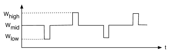
To get some intuition behind the working of this algorithm, consider the following simple example. Suppose can take three possible values from the set where . Similarly, can take three possible values in where and does not depend on . We assume that the workload process evolves in a frame-based periodic fashion. Specifically, in every odd numbered frame, for all except the last slot of the frame when . In every even numbered frame, for all except the last slot of the frame when . This is illustrated in Fig. 3. The process evolves similarly, such that when , when , and when .
In the following, we assume a frame size of slots with , , and units. Also, , , and dollars. Finally, , , , and we vary . In this example, intuitively, an optimal algorithm that knows the workload and unit cost process beforehand would recharge the battery as much as possible when and discharge it as much as possible when . In fact, it can be shown that the following strategy is feasible and achieves minimum average cost:
- •
If , then , , .
- •
If , then , , .
- •
If , then , , .
The time average cost resulting from this strategy can be easily calculated and is given by dollars/slot for all . Also, we note that the cost resulting from an algorithm that does not use the battery in this example is given by dollars/slot.
Now we simulate the dynamic algorithm for this example for different values of for slots ( frames). The value of is chosen to be (this choice will become clear in Sec. V-B when we relate to the battery capacity). Note that the number of slots for which a fully charged battery can sustain the data center at maximum load is .
| 20 | 30 | 40 | 50 | 75 | 100 | |
|---|---|---|---|---|---|---|
| 0 | 1.25 | 2.5 | 3.75 | 6.875 | 10.0 | |
| Avg. Cost | 94.0 | 92.5 | 91.1 | 88.5 | 88.0 | 87.0 |
In Table I, we show the time average cost achieved for different values of . It can be seen that as increases, the time average cost approaches the optimal value. (This behavior will be formalized in Theorem 1) This is remarkable given that the dynamic algorithm operates without any knowledge of the future workload and cost processes. To examine the behavior of the dynamic algorithm in more detail, we fix and look at the sample paths of the control decisions taken by the optimal offline algorithm and the dynamic algorithm during the first slots. This is shown in Figs. 4 and 5. It can be seen that initially, the dynamic tends to perform suboptimally. But eventually it learns to make close to optimal decisions.


It might be tempting to conclude from this example that an algorithm based on a price threshold is optimal. Specifically, such an algorithm makes a recharge vs. discharge decision depending on whether the current price is smaller or larger than a threshold. However, it is easy to construct examples where the dynamic algorithm outperforms such a threshold based algorithm. Specifically, suppose that the process takes values from the interval uniformly at random every slot. Also, suppose takes values from the set dollars uniformly at random every slot. We fix the other parameters as follows: , , , and . We then simulate a threshold based algorithm for different values of the threshold in the set and select the one that yields the smallest cost. This was found to be dollars/slot. We then simulate the dynamic algorithm for slots with and it yields an average cost of dollars/slot. We also note that the cost resulting from an algorithm that does not use the battery in this example is given by dollars/slot.
We now establish two properties of the structure of the optimal solution to P3 that will be useful in analyzing its performance later.
Lemma 2
The optimal solution to P3 has the following properties:
- 1.
If , then the optimal solution always chooses .
- 2.
If , then the optimal solution always chooses .
Proof:
See Appendix A. ∎
V-A Solving P3
In general, the complexity of solving P3 depends on the structure of the unit cost function . For many cases of practical interest, P3 is easy to solve and admits closed form solutions that can be implemented in real time. We consider two such cases here. Let denote the value of the objective in P3 when there is no recharge or discharge. Thus .
V-A1 does not depend on
Suppose that depends only on and not on . We can rewrite the expression in the objective of P3 as . Then, the optimal solution has the following simple threshold structure.
- 1.
If , then so that there is no recharge and we have the following two cases:
- (a)
If , then discharge as much as possible, so that we get , .
- (b)
Else, draw all power from the grid. This yields and .
- (a)
- 2.
Else if , then so that there is no discharge and we have the following two cases:
- (a)
If , then recharge as much as possible. This yields and .
- (b)
Else, draw all power from the grid. This yields and .
- (a)
We will show that this solution is feasible and does not violate the finite battery constraint in Sec. V-C.
V-A2 convex, increasing in
Next suppose for each , is convex and increasing in . For example, may have the form where for all . In this case, P3 becomes a standard convex optimization problem in a single variable and can be solved efficiently. The full solution is provided in Appendix E.
V-B Performance Theorem
We first define an upper bound on the maximum value that can take in our algorithm.
| (19) |
Then we have the following result.
Theorem 1
(Algorithm Performance) Suppose the initial battery charge level satisfies . Then implementing the algorithm above with any fixed parameter such that for all results in the following performance guarantees:
- 1.
The queue is deterministically upper and lower bounded for all as follows:
(20) - 2.
The actual battery level satisfies for all .
- 3.
All control decisions are feasible.
- 4.
If and are i.i.d. over slots, then the time-average cost under the dynamic algorithm is within of the optimal value:
(21) where is a constant given by and is the optimal solution to P1 under any feasible control algorithm (possibly with knowledge of future events).
Theorem 1 part shows that by choosing larger , the time-average cost under the dynamic algorithm can be pushed closer to the minimum possible value . However, limits how large can be chosen.
V-C Proof of Theorem 1
Here we prove Theorem 1.
Proof:
(Theorem 1 part ) We first show that (20) holds for . We have that
| (22) |
Using the definition (16), we have that . Using this in (22), we get:
This yields
Now suppose (20) holds for slot . We will show that it also holds for slot . First, suppose . Then, from Lemma 2, we have that . Thus, using (17), we have that . Next, suppose . Then, the maximum possible increase is so that . Now for all such that , we have that . This follows from the definition (19) and the fact that . Thus, we have .
Next, suppose . Then, from Lemma 2, we have that . Thus, using (17) we have that . Next, suppose . Then the maximum possible decrease is so that for this case as well. This shows that . Combining these two bounds proves (20). ∎
Proof:
(Theorem 1 parts and ) Part directly follows from (20) and (16). Using in the lower bound in (20), we have: , i.e., . Similarly, using in the upper bound in (20), we have: , i.e., .
Part now follows from part and the constraint on in P3. ∎
Proof:
(Theorem 1 part ) We make use of the technique of Lyapunov optimization to show (21). We start by defining a Lyapunov function as a scalar measure of congestion in the system. Specifically, we define the following Lyapunov function: . Define the conditional -slot Lyapunov drift as follows:
| (23) |
Using (17), can be bounded as follows (see Appendix B for details):
| (24) |
where . Following the Lyapunov optimization framework, we add to both sides of (24) the penalty term to get the following:
| (25) |
Using the relation , we can rewrite the above as:
| (26) |
Comparing this with P3, it can be seen that given any queue value , our control algorithm is designed to minimize the right hand side of (26) over all possible feasible control policies. This includes the optimal, stationary, randomized policy given in Lemma 1. Then, plugging the control decisions corresponding to the stationary, randomized policy, it can be shown that:
Taking the expectation of both sides and using the law of iterated expectations and summing over , we get:
Dividing both sides by and taking limit as yields:
where we have used the fact that is finite and that is non-negative. ∎
VI Extensions to Basic Model
In this section, we extend the basic model of Sec. III to the case where portions of the workload are delay-tolerant in the sense they can be postponed by a certain amount without affecting the utility the data center derives from executing them. We refer to such postponement as buffering the workload. Specifically, we assume that the total workload consists of both delay tolerant and delay intolerant components. Similar to the workload in the basic model, the delay intolerant workload cannot be buffered and must be served immediately. However, the delay tolerant component may be buffered and served later. As an example, data centers run virus scanning programs on most of their servers routinely (say once per day). As long as a virus scan is executed once a day, their purpose is served - it does not matter what time of the day is chosen for this. The ability to delay some of the workload gives more opportunities to reduce the average power cost in addition to using the battery. We assume that our data center has system mechanisms to implement such buffering of specified workloads.
In the following, we will denote the total workload generated in slot by . This consists of the delay tolerant and intolerant components denoted by and respectively, so that for all . Similar to the basic model, we use to denote the total power drawn from the grid, the total power used to recharge the battery and the total power discharged from the battery in slot , respectively. Thus, the total amount available to serve the workload is given by . Let denote the fraction of this that is used to serve the delay tolerant workload in slot . Then the amount used to serve the delay intolerant workload is . Note that the following constraint must be satisfied every slot:
| (27) |

We next define as the unfinished work for the delay tolerant workload in slot . The dynamics for can be expressed as:
| (28) |
For the delay intolerant workload, there are no such queues since all incoming workload must be served in the same slot. This means:
| (29) |
The block diagram for this extended model is shown in Fig. 6. Similar to the basic model, we assume that for , varies randomly in an i.i.d. fashion, taking values from a set of non-negative values. We assume that for all . We also assume that and for all . We further assume that . We use the same model for battery and unit cost as in Sec. III.
Our objective is to minimize the time-average cost subject to meeting all the constraints (such as finite battery size and (29)) and ensuring finite average delay for the delay tolerant workload. This can be stated as:
| Finite average delay for |
Similar to the basic model, we consider the following relaxed problem:
| (30) | ||||
| (31) |
where is the time average expected queue backlog for the delay tolerant workload and is defined as:
| (32) |
Let and denote the optimal value for problems P4 and P5 respectively. Since P5 is less constrained than P4, we have that . Similar to Lemma 1, the following holds:
Lemma 3
(Optimal Stationary, Randomized Policy): If the workload process and auxiliary process are i.i.d. over slots, then there exists a stationary, randomized policy that takes control decisions every slot purely as a function (possibly randomized) of the current state while satisfying the constraints (29), (2), (5), (9), (27) and providing the following guarantees:
| (33) | ||||
| (34) | ||||
| (35) |
where the expectations above are with respect to the stationary distribution of and the randomized control decisions.
Proof:
This result follows from the framework in [8, 9] and is omitted for brevity. ∎The condition (34) only guarantees queueing stability, not bounded worst case delay. We will now design a dynamic control algorithm that will yield bounded worst case delay while guaranteeing average cost that is within of .
VI-A Delay-Aware Queue
In order to provide worst case delay guarantees to the delay tolerant workload, we will make use of the technique of -persistent queue [19]. Specifically, we define a virtual queue as follows:
| (36) |
where is a parameter to be specified later, is an indicator variable that is if and else, and . The objective of this virtual queue is to enable the provision of worst-case delay guarantee on any buffered workload . Specifically, if any control algorithm ensures that and for all , then the worst case delay can be bounded. This is shown in the following:
Lemma 4
(Worst Case Delay) Suppose a control algorithm ensures that and for all , where and are some positive constants. Then the worst case delay for any delay tolerant workload is at most slots where:
| (37) |
Proof:
Consider a new arrival in any slot . We will show that this is served on or before time . We argue by contradiction. Suppose this workload is not served by . Then for all slots , it must be the case that (else would have been served before ). This implies that and using (36), we have:
Summing for all , we get:
Using the fact that and , we get:
| (38) |
Note that by (28), is part of the backlog . Since and since the service is FIFO, it will be served on or before time whenever at least units of power is used to serve the delay tolerant workload during the interval . Since we have assumed that is not served by , it must be the case that . Using this in (38), we have:
This implies that , that contradicts the definition of in (37). ∎
In Sec. VI-D, we will show that there are indeed constants such that the dynamic algorithm ensures that for all .
VI-B Optimal Control Algorithm
We now present an online control algorithm that approximately solves P4. Similar to the algorithm for the basic model, this algorithm also makes use of the following queueing state variable to track the battery charge level and is defined as follows:
| (39) |
where is a constant to be specified in (44). Recall that denotes the actual battery charge level in slot and evolves according to (3). It can be seen that is simply a shifted version of and its dynamics is given by:
| (40) |
We will show that this definition enables our algorithm to ensure that the constraint (4) is met. We are now ready to state the dynamic control algorithm. Let be the system state in slot . Define as the queue state that includes the workload queue as well as auxiliary queues. Then the dynamic algorithm chooses control decisions and as the solution to the following optimization problem:
where is a control parameter that affects the distance from optimality. Let and denote the optimal solution to P6. Then, the dynamic algorithm allocates power to service the delay intolerant workload and the remaining is used for the delay tolerant workload.
After computing these quantities, the algorithm implements them and updates the queueing variable according to (40). This process is repeated every slot. Note that in solving P6, the control algorithm only makes use of the current system state values and does not require knowledge of the statistics of the workload or unit cost processes.
We now establish two properties of the structure of the optimal solution to P6 that will be useful in analyzing its performance later.
Lemma 5
The optimal solution to P6 has the following properties:
- 1.
If , then the optimal solution always chooses .
- 2.
If (where is specified in (44)), then the optimal solution always chooses .
Proof:
See Appendix C. ∎
VI-C Solving P6
Similar to P3, the complexity of solving P6 depends on the structure of the unit cost function . For many cases of practical interest, P6 is easy to solve and admits closed form solutions that can be implemented in real time. We consider one such case here.
VI-C1 does not depend on
For notational convenience, let and .
Let denote the optimal value of the objective in P6 when there is no recharge or discharge. When does not depend on , this can be calculated as follows: If , then . Else, .
Next, let denote the optimal value of the objective in P6 when the option of recharge is chosen, so that . This can be calculated as follows:
- 1.
If , then .
- 2.
If , then .
- 3.
If , then .
- 4.
If , then we have two cases:
- (a)
If , then .
- (b)
If , then .
- (a)
Finally, let denote the optimal value of the objective in P6 when when the option of discharge is chosen, so that . This can be calculated as follows:
- 1.
If , then .
- 2.
If , then .
- 3.
If , then .
- 4.
If , then we have two cases:
- (a)
If , then .
- (b)
If , then .
- (a)
After computing , we pick the mode that yields the highest value of the objective and implement the corresponding solution.
VI-D Performance Theorem
We define an upper bound on the maximum value that can take in our algorithm for the extended model.
| (41) |
Then we have the following result.
Theorem 2
(Algorithm Performance) Suppose , and the initial battery charge level satisfies . Then implementing the algorithm above with any fixed parameter such that and a parameter such that for all results in the following performance guarantees:
- 1.
The queues and are deterministically upper bounded by and respectively for all where:
(42) (43) Further, the sum is also deterministically upper bounded by where
(44) - 2.
The queue is deterministically upper and lower bounded for all as follows:
(45) - 3.
The actual battery level satisfies for all .
- 4.
All control decisions are feasible.
- 5.
The worst case delay experienced by any delay tolerant request is given by:
(46) - 6.
If and are i.i.d. over slots, then the time-average cost under the dynamic algorithm is within of the optimal value:
(47) where is a constant given by and is the optimal solution to P4 under any feasible control algorithm (possibly with knowledge of future events).
Thus, by choosing larger , the time-average cost under the dynamic algorithm can be pushed closer to the minimum possible value . However, this increases the worst case delay bound yielding a utility-delay tradeoff. Also note that limits how large can be chosen.
Proof:
See Appendix D. ∎


VII Simulation-based Evaluation
We evaluate the performance of our control algorithms using both synthetic and real pricing data. To gain insights into the behavior of our algorithms and to compare with the optimal offline solution, we first consider the basic model and use a simple periodic unit cost and workload process as shown in Figs. 7 and 8. These values repeat every hours and the unit cost does not depend on . From Fig. 7, it can be seen that and . Further, we have that . We assume a slot size of minute so that the control decisions on are taken once every minute. We fix the parameters MW-slot, MW-slot, . We now simulate the basic control algorithm of Sec. V-A1 for different values of and with . For each , the simulation is performed for a duration of weeks.
In Fig. 9, we plot the average cost per hour under the dynamic algorithm for different values of battery size . It can be seen that the average cost reduces as is increased and converges to a fixed value for large , as suggested by Theorem 1. For this simple example, we can compute the minimum possible average cost per hour (over all battery sizes) and this is given by which is also the value to which the dynamic algorithm converges as is increased. Moreover, in this example, we can also compute the optimal offline cost for each value of . These also also plotted in Fig. 9. It can be seen that, for each , the dynamic algorithm performs quite close to the corresponding optimal value, even for smaller values of . Note that Theorem provides such guarantees only for sufficiently large values of . Finally, the average cost per hour when no battery is used is given by .

We next consider a six-month data set of average hourly spot market prices for the Los Angeles Zone LA1 obtained from CAISO [6]. These prices correspond to the period 01/01/200506/30/2005 and each value denotes the average price of 1 MW-Hour of electricity. A portion of this data corresponding to the first week of January is plotted in Fig. 1. We fix the slot size to 5 minutes so that control decisions on , etc. are taken once every 5 minutes. The unit cost obtained from the data set for each hour is assumed to be fixed for that hour. Furthermore, we assume that the unit cost does not depend on the total power drawn .
In our experiments, we assume that the data center receives workload in an i.i.d fashion. Specifically, every slot, takes values from the set [0.1,1.5] MW uniformly at random. We fix the parameters and to MW-slot, , and . Also, MW. We now simulate four algorithms on this setup for different values of . The length of time the battery can power the data center if the draw were starting from fully charged battery is given by slots, each of length minutes. We consider the following four control techniques: (A) “No battery, No WP,” which meets the demand in every slot using power from the grid and without postponing any workload, (B) “Battery, No WP,” which employs the algorithm in the basic model without postponing any workload, (C) “No Battery, WP,” which employs the extended model for WP but without any battery, and (D) “Complete,” the complete algorithm of the extended model with both battery and WP. For (C) and (D), we assume that during every slot, half of the total workload is delay-tolerant.
We simulate these algorithms to obtain the total cost over the month period for MW-slot. For (B), we use while for (C) and (D), we use with . Note that an increased battery capacity should have no effect on the performance under (C). In order to get a fair comparison with the other schemes, we assume that the worst case delay guarantee that case (C) must provide for the delay tolerant traffic is the same as that under (D).
Fig. 10 plots the total cost under these schemes over the month period. In Table II, we show the ratio of the total cost under schemes (B), (C), (D) to the total cost under (A) for these values of over the month period. It can be seen that (D) provides the most cost savings over the baseline case.

| 15 | 30 | 50 | |
|---|---|---|---|
| Battery, No WP | 95% | 92% | 89% |
| WP, No Battery | 96% | 92% | 88% |
| WP, Battery | 92% | 85% | 79% |
VIII Conclusions and Future Work
In this paper, we studied the problem of opportunistically using energy storage devices to reduce the time average electricity bill of a data center. Using the technique of Lyapunov optimization, we designed an online control algorithm that achieves close to optimal cost as the battery size is increased.
We would like to extend our current framework along several important directions including: (i) multiple utilities (or captive sources such as DG) with different price variations and availability properties (e.g., certain renewable sources of energy are not available at all times), (ii) tariffs where the utility bill depends on peak power draw in addition to the energy consumption, and (iii) devising online algorithms that offer solutions whose proximity to the optimal has a smaller dependence on battery capacity than currently. We also plan to explore implementation and feasibility related concerns such as: (i) what are appropriate trade-offs between investments in additional battery capacity and cost reductions that this offers? (ii) what is the extent of cost reduction benefits for realistic data center workloads? and (iii) does stored energy make sense as a cost optimization knob in other domains besides data centers? Our technique could be viewed as a design tool which, when parameterized well, can assist in determining suitable configuration parameters such as battery size, usage rules-of-thumb, time-scale at which decisions should be made, etc. Finally, we believe that our work opens up a whole set of interesting issues worth exploring in the area of consumer-end (not just data centers) demand response mechanisms for power cost optimization.
Acknowledgments
This work was supported in part by the NSF Career grant CCF-0747525.
References
- [1] S. Park, W. Jiang, Y. Zhou, and S. Adve, “Managing energy-performance tradeoffs for multithreaded applications on multiprocessor architectures,” in Proc. ACM SIGMETRICS, 2007.
- [2] Q. Zhu, F. David, C. Devaraj, Z. Li, Y. Zhou, and P. Cao, “Reducing energy consumption of disk storage using power-aware cache management,” in Proc. HPCA, 2004.
- [3] S. Gurumurthi, A. Sivasubramaniam, M. Kandemir, and H. Franke, “Drpm: Dynamic speed control for power management in server class disks,” in Proc. ISCA ’03, 2003.
- [4] A. R. Lebeck, X. Fan, H. Zeng, and C. Ellis, “Power aware page allocation,” SIGOPS Oper. Syst. Rev., vol. 34, pp. 105–116, Nov. 2000.
- [5] J. S. Chase, D. C. Anderson, P. N. Thakar, A. M. Vahdat, and R. P. Doyle, “Managing energy and server resources in hosting centers,” SIGOPS Oper. Syst. Rev., vol. 35, pp. 103–116, Oct. 2001.
- [6] California ISO Open Access Same-time Information System (OASIS) Hourly Average Energy Prices. http://oasisis.caiso.com.
- [7] D. P. Bertsekas, Dynamic Programming and Optimal Control, vols. 1 and 2. Athena Scientific, 2007.
- [8] L. Georgiadis, M. J. Neely, and L. Tassiulas, “Resource allocation and cross-layer control in wireless networks,” Found. and Trends in Networking, vol. 1, pp. 1–144, 2006.
- [9] M. J. Neely, Stochastic Network Optimization with Application to Communication and Queueing Systems. Morgan & Claypool, 2010.
- [10] A. Bar-Noy, M. P. Johnson, and O. Liu, “Peak shaving through resource buffering,” in Proc. WAOA, 2008.
- [11] A. Bar-Noy, Y. Feng, M. P. Johnson, and O. Liu, “When to reap and when to sow: Lowering peak usage with realistic batteries,” in Proc. 7th International Conference on Experimental Algorithms, 2008.
- [12] K. Le, R. Bianchini, M. Martonosi, and T. Nguyen, “Cost- and energy-aware load distribution across data centers,” in Workshop on Power-Aware Computing and Systems (HOTPOWER), 2009.
- [13] A. Qureshi, R. Weber, H. Balakrishnan, J. Guttag, and B. Maggs, “Cutting the electric bill for internet-scale systems,” in Proc. SIGCOMM, 2009.
- [14] M. Gatzianas, L. Georgiadis, and L. Tassiulas, “Control of wireless networks with rechargeable batteries,” IEEE Trans. Wireless. Comm., vol. 9, pp. 581–593, Feb. 2010.
- [15] D. Linden and T. B. Reddy, Handbook of Batteries. McGraw Hill Handbooks, 2002.
- [16] Lead-acid batteries: Lifetime vs. Depth of discharge. http://www.windsun.com/Batteries/Battery_FAQ.htm.
- [17] M. Marwah, P. Maciel, A. Shah, R. Sharma, T. Christian, V. Almeida, C. Araújo, E. Souza, G. Callou, B. Silva, S. Galdino, and J. Pires, “Quantifying the sustainability impact of data center availability,” SIGMETRICS Perform. Eval. Rev., vol. 37, pp. 64–68, March 2010.
- [18] U. Hoelzle and L. A. Barroso, The Datacenter as a Computer: An Introduction to the Design of Warehouse-Scale Machines. Morgan and Claypool Publishers, 2009.
- [19] M. J. Neely, A. S. Tehrani, and A. G. Dimakis, “Efficient algorithms for renewable energy allocation to delay tolerant consumers,” in Proc. IEEE SmartGridComm, 2010.
Appendix A -Proof of Lemma 2
We can rewrite the expression in the objective of P3 as . To show part , suppose when , so that we have , , , and . Then the value of the objective is given by:
where the last step follows by noting that when and that in non-negative and non-decreasing in . The last expression denotes the value of the objective when and all demand is met using power drawn from the grid and is smaller. This shows that when , then the optimal solution cannot choose .
Next, to show part , suppose when , so that we have , , and . Then the value of the objective is given by:
where in the last step, we used the property (10) together with the fact that . The last expression denotes the value of the objective when and all demand is met using power drawn from the grid and is smaller. This shows that when , then the optimal solution cannot choose .
Appendix B - Proof of Bound (24)
Squaring both sides of (17), dividing by , and rearranging yields:
Now note that under any feasible algorithm, at most one of and can be non-zero. Further, since for all , we have:
Taking conditional expectations of both sides given , we have: .
IX Proof of Lemma 5
Suppose and . Then, we have that . After rearranging, the value of the objective of P6 can be expressed as:
where we used the inequalities and . The first follows from the non-negative and non-decreasing property of in . The second follows by noting that . Now note that the right hand side denotes the value of the objective when power is drawn from the grid and the battery is not recharged or discharged. This is a feasible option since by choosing , we have that . This shows that when , is not optimal. This shows part .
Next, suppose and ,
.
Then, we have that
.
We consider two cases:
(1) : After rearranging, the value of the objective of P6 can be expressed as:
where we used the fact that and . Using the property (10), we have:
Using this in the inequality above, we have:
Note that the last term denotes the value of objective when power
is drawn from the grid and the battery is not recharged or
discharged. This is a feasible option since by choosing
, we have that
.
This shows that for this case, when , is not optimal.
(2) : The value of the objective of P6 is given by:
where we used the fact that since and (Theorem 2 part ), we have . The last term in the inequality above denotes the value of the objective when power is drawn from the grid and the battery is not recharged or discharged. To see that this is feasible, note that we need where must be . Since , this implies:
where we used the fact that . Now since , the last term above is , so that choosing and is a feasible option. This shows that for this case as well, is not optimal.
Appendix D - Proof of Theorem 2, parts 2-6
Here, we prove parts of Theorem 2.
Proof:
(Theorem 2 part ) We first show (42). Clearly, (42) holds for . Now suppose it holds for slot . We will show that it also holds for slot . First suppose . Then, by (28), the most that can increase in one slot is so that . Next, suppose . Now consider the terms involving in the objective of P6: . Since , using property (10), we have:
Thus, the optimal solution to problem P6 chooses . Now, let and denote the other control decisions by the optimal solution to P6. Then the amount of power remaining for the data center (after recharging or discharging the battery) is . Out of this, a fraction is used to serve the delay intolerant workload. Thus:
Using this, and the fact that , we have:
where we used the fact that . Thus, using (28), it can be seen that the amount of new arrivals to cannot exceed the total service and this yields .
(43) can be shown by similar arguments. Clearly, (43) holds for . Now suppose it holds for slot . We will show that it also holds for slot . First suppose . Then, by (36), the most that can increase in one slot is so that . Next, suppose . Then, by a similar argument as before, the optimal solution to problem P6 chooses Now, let and denote the other control decisions by the optimal solution to P6. Then the amount of power remaining for the data center is . Out of this, a fraction is used for the delay intolerant workload. Thus:
Using this, and the fact that , we have:
where we used the fact that and . Thus, using (36), it can be seen that the amount of new arrivals to cannot exceed the total service and this yields .
(44) can be shown by similar arguments and the proof is omitted for brevity. ∎
Proof:
(Theorem 2 part ) We first show that (45) holds for . Using the definition of from (39), we have that . Since , we have:
Next, we have that , so that:
Combining these two shows that .
Now suppose (45) holds for slot . We will show that it also holds for slot . First, suppose . Then, from Lemma 5, we have that . Thus, using (40) we have that . Next, suppose . Then, the maximum possible increase is so that . Now for all such that , we have that . This follows from the definition (41) and the fact that . Using this, we have for this case as well. This establishes that .
Next, suppose . Then, from Lemma 5, we have that . Thus, using (40) we have that . Next, suppose . Then, the maximum possible decrease is so that for this case as well. This shows that . Combining these two bounds proves (45). ∎
Proof:
(Theorem 2 parts and ) Part directly follows from (45) and (39). Using in the lower bound in (45), we have:
Similarly, using in the upper bound in (45), we have:
Part now follows from part and the constraint on in P6. ∎
Proof:
Proof:
(Theorem 2 part ) We use the following Lyapunov function: . Define the conditional -slot Lyapunov drift as follows:
| (48) |
Using (28), (36), (40), the drift + penalty term can be bounded as follows:
| (49) |
where . Comparing this with P6, it can be seen that given any queue value , our control algorithm is designed to minimize the right hand side of (49) over all possible feasible control policies. This includes the optimal, stationary, randomized policy given in Lemma 3. Using the same argument as before, we have the following:
Taking the expectation of both sides and using the law of iterated expectations and summing over , we get
Dividing both sides by and taking limit as yields:
where we used the fact that is finite and that is non-negative. ∎
Appendix E - Full Solution for Convex, Increasing
Let be the derivative of with respect to . Also, let denote the solution to the equation and . Then, the optimal solution can be obtained as follows:
- 1.
If , then and we have the following two cases:
- (a)
If , then , .
- (b)
Else, draw all power from the grid. This yields and .
- (a)
- 2.
If , then and we have the following two cases:
- (a)
If , then , .
- (b)
Else, draw all power from the grid. This yields and .
- (a)
- 3.
If , then and we have the following two cases:
- (a)
If , then , .
- (b)
Else, draw all power from the grid. This yields and .
- (a)
- 4.
If , then and we have the following two cases:
- (a)
If , then , .
- (b)
Else, draw all power from the grid. This yields and .
- (a)