10.1080/0001873YYxxxxxxxx \issn1460-6976 \issnp0001-8732 \jvol00 \jnum00 2011 \jmonthJune
The Bond-Algebraic Approach to Dualities
Abstract
An algebraic theory of dualities is developed based on the notion of bond algebras. It deals with classical and quantum dualities in a unified fashion explaining the precise connection between quantum dualities and the low temperature (strong-coupling)/high temperature (weak-coupling) dualities of classical statistical mechanics (or (Euclidean) path integrals). Its range of applications includes discrete lattice, continuum field, and gauge theories. Dualities are revealed to be local, structure-preserving mappings between model-specific bond algebras that can be implemented as unitary transformations, or partial isometries if gauge symmetries are involved. This characterization permits to search systematically for dualities and self-dualities in quantum models of arbitrary system size, dimensionality and complexity, and any classical model admitting a transfer matrix or operator representation. In particular, special dualities like exact dimensional reduction, emergent, and gauge-reducing dualities that solve gauge constraints can be easily understood in terms of mappings of bond algebras. As a new example, we show that the Higgs model is dual to the extended toric code model in any number of dimensions. Non-local transformations like dual variables and Jordan-Wigner dictionaries are algorithmically derived from the local mappings of bond algebras. This permits to establish a precise connection between quantum dual and classical disorder variables. Our bond-algebraic approach goes beyond the standard approach to classical dualities, and could help resolve the long standing problem of obtaining duality transformations for lattice non-Abelian models. As an illustration, we present new dualities in any spatial dimension for the quantum Heisenberg model. Finally, we discuss various applications including location of phase boundaries, spectral behavior and, notably, we show how bond-algebraic dualities help constrain and realize fermionization in an arbitrary number of spatial dimensions.
CONTENTS
1. Introduction: The power of dualities 2. Traditional approaches to dualities 2.1. Dualities in perspective: What is a duality? 2.2. The traditional approach to quantum dualities 3. Bond-algebraic approach to quantum dualities 3.1. Bond algebras and the concept of locality 3.2. Some mathematical aspects of bond algebras 3.3. Dualities as isomorphisms of bond algebras 3.4. Connection to the traditional approach: Determination of dual variables 3.5. Abelian versus non-Abelian dualities: the Heisenberg model 3.6. Exact dualities for finite systems 3.7. Dualities as unitary transformations 3.8. Dualities and quantum symmetries 3.9. Order and disorder variables for self-dual models 3.10. Emergent dualities 3.11. Elimination of gauge symmetries by bond-algebraic dualities 3.12. Unifying classical and quantum dualities 4. Quantum self-dualities by example: Lattice models 4.1. Self-dualities in the Potts, vector Potts, and clock models 4.2. Dualities in some limits and related approximations 4.3. The Xu-Moore model 5. Quantum dualities by example: Lattice models 5.1. XY/solid-on-solid models 5.2. Xu-Moore/planar orbital compass models 5.3. Two-dimensional gauge/vector Potts models 5.4. Two-dimensional compact QED and XY models 5.5. Toric code/ Higgs models 6. Bond-algebraic dualities in quantum field theory 6.1. One-dimensional free and externally coupled bosonic field, and the Kibble model 6.2. The Luttinger model 6.3. QED without sources, compact QED, and gauge theories 6.4. QED without vector potential 6.5. Abelian and Higgs, and Stückelberg models 6.6. The self-dual Stückelberg model 6.7. Field theory and dimensional reduction 7. Bond-algebraic approach to classical dualities 7.1. The classical Ising model in the Utiyama lattice 7.2. The classical vector Potts model 7.3. The classical eight-vertex model 7.4. Classical dualities in and dimensions 7.5. Dualities for continuum models of classical statistical mechanics 7.5 Classical disorder variables from quantum ones 8. Applications of dualities 8.1. Self-dualities and phase transitions 8.2. Correlation functions 8.3. Fermionization as a duality 8.4. Self-dualities and quantum integrability 8.5. Duality, topological quantum order, and dimensional reduction 9. Appendices Appendix A: Duality by Fourier transformation Appendix B: Conditions for spectral equivalence Appendix C: Lattice quantum field theory Appendix D: Bond-algebraic dualities in finite-size systems Appendix E: Classical Poisson dualities Appendix F: Exponential of operators in the Weyl group algebra
keywords
quantum and classical dualities; statistical mechanics; field theory; gauge theories; dimensional reduction; phase transitions; fermionization; bond algebras, operator algebras1 Introduction: The power of dualities
The term duality is pervasive in physics, mathematics and philosophy. In general, a duality connects and contrasts two aspects or realizations of a given entity. In this article we will be concerned only with dualities in physics. These are specific mathematical transformations that we will uncover as we proceed connecting seemingly unrelated physical phenomena.
Over time, dualities have appeared in various guises in nearly all disciplines of physics [1]. The electromagnetic (EM) duality of Maxwell’s equations in the absence of sources, noticed by Heaviside in 1884, is probably the oldest well-known duality in modern physics. Later, the wave-particle duality of quantum mechanics [2] became a fundamental tenet of the modern physical description of reality. This Fourier transform-based duality has since appeared in numerous arenas, including in recent years various branches of quantum statistical mechanics and field theory (see, for example, [3]), and it is likely to continue to play an ever increasing role. Kramers and Wannier introduced dualities in statistical mechanics in their foundational 1941 paper [4]. These authors discovered an elegant relation between the two-dimensional classical Ising model on a square lattice at high temperature, and the same model at low temperature (hence the origin of the name “self-duality” in this case), and used it to determine that model’s exact critical temperature some years before Onsager [5] published its exact solution. This first quantitative success was followed by other similar ones, and so dualities became a standard tool in statistical mechanics since they could also provide qualitative insight. The spectacular cross-fertilization between statistical mechanics and quantum field theory (QFT) of the 1970’s brought dualities to the attention of high energy theorists, and soon it became apparent that dualities in QFT combined features of the EM and statistical mechanics dualities while retaining their distinct capability to produce weakly-coupled representations of strongly-coupled problems.
Dualities can provide reliable qualitative or even exact quantitative information about systems that need not be exactly solvable, partly because they can put constraints on the phase boundaries and the exact location of some critical or multi-critical points. Thus (self-)dualities have been essential for investigating the phase diagrams of numerous models in statistical mechanics and field theory [6, 7]. This aspect encompasses some of the most spectacular applications of dualities, and constitutes the legacy of Kramers and Wannier. However, dualities can become even more potent when fused with other tools, such as perturbation theory. A case in point is the AdS-CFT correspondence, a topic that remains the focus of intense research efforts. Since its original formulation in high energy physics [8, 9, 10, 11], this conjecture of a duality between a weakly-coupled five-dimensional gravity theory (on an Anti de Sitter (AdS) background) and a strongly-coupled four-dimensional conformal field theory (CFT) has been generalized and exploited in other branches of physics. At present, the range of applications of the AdS-CFT correspondence includes problems as diverse as electronic transport properties [12], quantum critical dynamics [13], and the physics of strongly coupled quark-gluon plasmas [14]. The efforts to apply the AdS-CFT correspondence to other strongly-coupled models continue, but the problem of pushing it beyond a conjecture into a rigorous mathematical statement remains. We think that turning the AdS-CFT correspondence into a mathematically rigorous duality is essential to understanding its potential generalizations.
These examples (old and new) attest to the power of dualities and justifies the efforts of numerous researchers to exploit them to address hard problems by simple, elegant means. This article is a self-contained exposition of extensive original developments, including many new dualities and self-dual models, in the general bond-algebraic theory of dualities first introduced in Reference [15] (bond algebras have also been employed in the analysis and spectral resolution of exactly solvable models [16, 17], but this application is not discussed in this paper). In the context of some specific models, quantum dualities have been well understood for many years. Reference [15] introduced a coherent framework supporting a systematic study of both quantum and classical dualities on an equal footing, and providing a systematic way to compute dual (disorder) variables. The new, unified, theory that emerges is rigorous, easy to use, algorithmic, and of practical significance to theoretical studies and numerical simulations. It has the potential to provide invaluable insight into a myriad of pressing problems that are beyond perturbation theory. Our theory of dualities rests on a single key observation: The bonds or interactions of a Hamiltonian or transfer matrix are more relevant to a duality transformation than the elementary degrees of freedom. Those bonds, or interaction terms, are organized into a bond algebra. In contrast, symmetries or properties of the elementary degrees of freedom are largely irrelevant from a duality mapping perspective [16, 15]. Our bond-algebraic approach to dualities may shed light on problems like the characterization and classification of collective (topological) excitations of lattice models, and the AdS-CFT correspondence [18], when complemented with recent developments in the theory of dimensional reduction [19, 20].
Hamiltonians that meet basic physical requirements like causality are usually realized by adding together (or integrating with a given measure in QFT) simple local or quasi-local operators, like few-body interactions and kinetic energy single-body operators. These operators (or some simple function of them) constitute the bond operators, or bonds for short. Together they generate, in a sense to be specified in Section 3.1, an operator von Neumann algebra that we call a bond algebra. Bond algebras are model-specific algebras of interactions that can be radically different from the algebras that embody elementary degrees of freedom like bosons, fermions, or spins. Our new theory states that dualities are structure-preserving mappings (homomorphisms) of bond algebras, that are typically local in the bonds. This purely algebraic characterization is physically meaningful because homomorphism of bond algebras are always equivalent to a unitary transformation (or, if gauge symmetries are involved, to a partial isometry) connecting the Hilbert spaces on which the two models connected by a duality are defined. Thus quantum dualities are revealed as unitary transformations, and dual models must share identical spectra and level degeneracies; that is, provided gauge symmetries are not involved. The precise connection between gauge symmetries and dualities will be one of the central themes of this paper.
Remarkably, these ideas can be extended to include classical dualities [15], thus unifying the theory of classical and quantum dualities in a way that had been overlooked up to now. The key is to notice that many problems in classical statistical physics can be formulated in terms of a transfer matrix or operator. In this context, physical requirements like locality become manifest in the multiplicative structure of the transfer matrix or operator, that will be in general a product of local or quasi-local bonds. Once the bonds are identified, the theory of dualities proceeds as before. Thus, a duality mapping for the bond algebra of the transfer matrix realizes a dual transfer matrix that determines a dual representation of the partition function . But, since dualities are unitary transformations, it follows that . This is, in short, the bond-algebraic approach to classical dualities. In this way one can show, for instance, that the self-duality of the two-dimensional classical Ising model [4, 21], and the self-duality of the quantum Ising chain [22] are two manifestations of a symmetry possessed by one and the same bond algebra. But more importantly, we will illustrate in this paper that the bond-algebraic approach has the potential to extend classical dualities beyond its present boundaries, as set for example in the reviews [6, 7] (see Appendix A). We think that this strongly indicates that our technique can be relevant to solving the open problem of constructing dual representations of non-Abelian lattice models, although so far we have only some examples to support this claim.
Bond algebras are most efficient in revealing dualities because they are model (Hamiltonian/transfer matrix)-specific, and thus capture, in the form of a local mapping, the precise information that makes two operators dual. This is different from techniques based on essentially fixed mappings, like generalized Jordan-Wigner transformations [23]. These transformations are isomorphisms (that we call dictionaries) connecting operator algebras (i.e., languages), typically representing elementary degrees of freedom. Since these dictionaries are insensitive to the specific structure of physical models, they can easily spoil important physical characteristics, as illustrated by standard fermionization in more than one space dimension. However, it is important to underscore that a bond algebra is not uniquely determined by the Hamiltonian/transfer matrix that motivates its definition, but rather by the choice of bond decomposition of those operators. Since that choice is not unique, (i) any single Hamiltonian may produce many different bond algebras, and (ii) any one bond algebra may be related to many different Hamiltonians. This flexibility is essential for classification purposes and to the success of our technique. It enables us to explore a variety of bond algebras for one and the same Hamiltonian/transfer matrix to capture its full range of dual representations. Similarly, it allow us to apply one and the same duality mapping to different problems. The self-duality for the spin XY model in a transverse field of Section 3.10.2 provides an example of the first observation (i) above. In this case, the self-duality emerges on a special line in coupling space, and it takes a special choice of bonds to generate the bond algebra that makes this self-duality apparent. The second observation (ii) is illustrated by the new dualities of Section 3.5 for the quantum Heisenberg model in any number of space dimensions . These dualities for a non-Abelian model are based on dualities for the (Abelian!) -dimensional quantum Ising model and highlight some difficulties with the standard notion of non-Abelian dualities [6]. They point to the fact that the concepts of symmetry and duality are quite often inaccurately related. While symmetries of a theory represent isomorphisms leaving the Hamiltonian invariant, (self-)dualities do not preserve the form of the theory, but rather preserve its spectrum and level degeneracies.
The relevance of bonds over elementary degrees of freedom is further emphasized by the fact that dualities are local transformations in terms of bonds, while they are non-local when described in terms of elementary degrees of freedom. This follows because one can invert the relations between bonds and elementary degrees of freedom to obtain the latter as non-local functions of the bonds. Once this is done, one can compute the action of the duality mapping on the elementary degrees of freedom, to obtain their dual image. Since dualities are structure-preserving mappings, these dual elementary degrees of freedom are guaranteed to be equivalent to the original ones. This systematic derivation of (non-local in general) dual variables (elementary degrees of freedom) from more basic, local objects is extremely important, not only because it establishes a bridge between the bond-algebraic and the traditional approach to quantum dualities, but also because dual variables can have a fundamental physical meaning as (generalized) disorder variables [24, 22].
Starting with any specific bond algebra, one can proceed to look systematically for its alternative realizations that feature local representations of the bond generators. Any of these realizations defines a duality (realizations that feature non-local representations of the bond generators can appear, but would typically be discarded in practice). This simple premise can lead to surprising results, as we will see often in this paper. Exact dimensional reduction can appear as a duality, and, as illustrated by our new derivation of the Jordan-Wigner transformation, statistical transmutation can appear as a duality too. Symmetry transmutation is also not unusual as illustrated for example by our new derivation of the duality between the XY and solid-on-solid (SoS) models, obtained here for the first time without invoking the Villain approximation (symmetry transmutation here refers to the fact that the symmetry group of the XY model is not isomorphic, but rather the Pontryagin dual of the symmetry group of the SoS model). But perhaps what is most surprising about bond-algebraic dualities is their capability to dispose of gauge symmetries, as we explain next.
Gauge symmetries are constraints on the state Hilbert space, encoded in a large set of local operators that commute with the Hamiltonian, and with any other (measurable) observable. Since bonds are in general measurable, local observables, they generate a bond algebra of gauge-invariant operators. This has the remarkable consequence that bond algebras of gauge models can have dual representations on state spaces of lower dimensionality (a fact that should not be confused with an emergent duality as described in Section 3.10). We call these dualities gauge-reducing; they map the original gauge model to a model with less, or simply without gauge symmetries, and are represented by homomorphisms of bond algebras, rather than isomorphisms. Unlike ordinary dualities that are unitarily implementable, gauge-reducing dualities are implemented by partial isometries (one can think of a partial isometry as a rectangular unitary matrix, that either maps a state to zero or to an isometric (equal norm) state). But in spite of these mathematical twists, dualities are just as easy to detect in gauge theories as in any other model. That is because, while gauge symmetries do affect the algebra of elementary degrees of freedom, they do not affect the algebraic relations between bonds. Thus bond-algebraic dualities may provide in some instances a practical solution to the problem of eliminating gauge constraints. This paper describes in detail the mathematics and multiple applications of these ideas to models with Abelian gauge symmetries. Non-Abelian gauge symmetries abide by the same principles but are technically more involved, so we defer their complete treatment to future publications.
This article contains many new results and is organized as follows. Section 2.1 starts with a discussion of the different physical contexts in which dualities have been introduced, followed in Section 2.2 by a more detailed discussion of what was known about quantum dualities prior to the publication of Reference [15], the so-called standard approach. These discussions should help the reader put the subject of dualities, and some of the problems they address, in perspective. Section 3 contains all the important formal developments related to the bond-algebraic approach to dualities. Overall it is devoted to quantum dualities and their intimate connection to classical dualities, mainly discussing every major new idea and mathematical technique that is of relevance. We start by studying bond algebras in Sections 3.1 and 3.2. Our new definition of quantum dualities as mappings of bond algebras is presented in Section 3.3, and the next section explains how the standard approach described in Section 2.2 follows immediately from the bond-algebraic formalism (determination of dual variables). Section 3.5 discusses critically the notion of non-Abelian duality, in the light of new dualities for the quantum Heisenberg model, and Section 3.6 develops new boundary conditions that preserve duality properties in finite size systems. Section 3.7 expands, in more concrete terms, on the connection between bond algebra mappings and unitary transformations. The remaining sections are devoted to deriving and explaining the precise relations between self-dualities, standard quantum symmetries, Section 3.8, and disorder variables, Section 3.9, and the novel concept of emergent duality, Section 3.10. Disorder variables can be systematically determined from bond-algebraic dual mappings and they share an interesting relation with topological excitations. Section 3.11 explains how bond-algebraic dualities afford a practical way to eliminate gauge symmetries completely, and finally Section 3.12 explains how many classical dualities follow from bond-algebraic techniques.
The rest of the article is dedicated to unveil old and discover new dualities in a broad spectrum of problems of physical relevance. There are so many examples that in the following we only indicate a few of them. Sections 4 and 5 exemplify the many ideas ideas and techniques developed in Section 3 with self-dualities and dualities in quantum lattice models, of arbitrary spatial dimensions, mainly of interest in condensed matter physics. For example, Section 5.5 describes a new duality for the extended Kitaev toric code model in arbitrary space dimensions to a well known model of Hamiltonian lattice field theory, the Abelian Higgs model [86]. The application of bond-algebraic techniques to QFT is developed in Section 6. Sometimes we show results directly in the continuum but we want to stress the fact that the lattice Hamiltonian formalism is the most convenient approach for interacting field theories. We study in full detail compact and non-compact versions of quantum electrodynamics in various spatial dimensions and make an attempt to introduce a version of quantum electrodynamics without vector potential. In Section 6.5 we introduce a new family of self-dual models related to the Abelian Higgs model, we prove the quantum Stückelberg model to be self-dual in two-dimensions in Section 6.6, and Section 6.7 discusses self-dual field theories that display the phenomenon of dimensional reduction of prime interest in the theory of topological quantum order [20].
Section 7 presents several problems of classical statistical mechanics whose duality properties are uncovered by our bond-algebraic approach. Section 7.1 describes duality properties of the Ising model in the Utiyama lattice, while the vector Potts model in two dimensions is not only studied in great detail in Section 7.2 but also it is shown how to modify it to make it self-dual for arbitrary couplings and states. Building upon these ideas we introduce a new self-dual -state approximation to four-dimensional lattice electrodynamics in Section 7.4. Section 7.3 establishes a link between the eight-vertex model (in its Ashkin-Teller representation) and the quantum anisotropic Heisenberg model, based on duality mappings rather than integrability. The general connection between quantum and classical disorder variables is discussed in Section 7.6. Finally, Section 8 presents several important applications and consequences of dualities. Those include general properties of the spectrum of self-dual theories and the way to extract exact relevant information in presence of phase transitions, and most importantly a new way to look at fermionization in arbitrary spatial dimensions as a general duality mapping. In particular, we demonstrate how the Jordan-Wigner transformation is a consequence of bond algebraic duality mappings when these are applied to nearest-neighbor spinless fermion and spin systems on a chain. We further show, how no such duality can map all (real-space) nearest-neighbor spinless Fermi hopping terms to all spin exchange terms on general lattices (and viceversa) in spatial dimensions . That is, in general, no extension of the Jordan-Wigner transformation that connects all such individual local terms can appear in higher dimensions. We show, however, that notwithstanding it is possible to fermionize spin systems in dimensions (such as the quantum Ising model) via a gauge reducing duality. Thus we further extend and formalize, via the systematics of bond algebras, the scope of known systems that can be fermionized. In Section 8.5 we examine the connection between the phenomenon of dimensional reduction and duality in the context of topological quantum order systems [20]. We also indicate the most natural way to classify these systems in terms of so-called -dimensional gauge-like symmetries as opposed to using a particular measure of entanglement since no single measure can uniquely characterize a quantum state.
The appendices, a total of five, contain not only technical details omitted in the text for pedagogical reasons but also some relevant mathematical expressions not found in the literature, so we advice the reader to consider consulting them if he or she wants to get a deeper understanding of the subject.
2 Traditional approaches to dualities
This short section discusses dualities in physics from a historical perspective. Mainstream, traditional ideas about dualities in field theory, classical statistical mechanics and quantum mechanics are summarized and illustrated with key examples.
2.1 Dualities in perspective: What is a duality?
The first appearance of the term duality can be traced back to the early days of electromagnetism as a field theory. In 1884, Heaviside recast Maxwell’s equations in vector form [25], in the absence of sources,
| (1) | |||||
(in rationalized Heaviside-Lorentz units, and the speed of light ), and pointed out that the duality
| (2) |
maps solutions of these equations to other solutions. This notion of duality stresses symmetries of the equations of motion showing that different physical quantities are interchangeable.
Two of Maxwell’s equations can be solved by introducing a four-vector potential (), that is related to and through the antisymmetric field-strength tensor
| (3) |
Then the remaining Maxwell’s equations read ()
| (4) |
This formalism is essential for well know reasons, but the (self-)duality of Maxwell’s equations is not readily reflected by Equation (4), partly because the gauge transformation, with arbitrary scalar function ,
| (5) |
leaves the EM field unchanged but renders unobservable. This motivates one of this paper’s central theme: the interplay between dualities and gauge symmetries.
A second, seemingly very different, concept of duality was developed in the early 1940s in the context of classical statistical mechanics. It originated in the work of Kramers and Wannier [4] on the two-dimensional () Ising model on a square lattice, with partition function
| (6) |
Here stands for a classical spin degree of freedom located on the vertex (site) , , of a square lattice with unit vectors , see Figure 2. The exchange constant is , with temperature and Boltzmann’s constant. Kramers and Wannier noticed that satisfies a relation
| (7) |
that, since
| (8) |
connects the high-temperature (weak ) behavior of the Ising model to its low temperature (strong ) behavior ( is a known, analytic (non-singular) proportionality factor). It follows that every singularity of at coupling must be matched by another singularity at a corresponding dual coupling , so that if has only one phase transition (one singularity) at a critical coupling , it must be located at the self-dual point . Then from Equation (8)
| (9) |
which determines the exact critical temperature of the Ising model (in units of ).
This spectacular result drew considerable attention to duality transformations, and soon after the publication of Reference [4], Wannier [26] showed how to obtain duality relations of the form
| (10) |
for Ising models defined on nearly arbitrary planar lattices . These transformations where dubbed dualities [26] because stands for the lattice dual to (dual here is used in the sense of old algebraic topology, see for instance, Reference [27], Chapter IV, Section 6.) Dual lattices are defined in Appendix A. We see from Equation (10) that the Ising model on a square lattice is self-dual partly because so is the square lattice, while the Ising model on a triangular lattice is dual to that same model on a hexagonal lattice (and viceversa). This last duality is part of a simple approach to determining these models’ critical temperature [28].
Potts extended the duality transformation of Wannier to some of the models now known under his name in his 1952 paper [29]. It was Wegner, however, who uncovered the general structure underlying dualities, by showing in his 1973 paper [30] that duality transformations could be obtained for a wide class of models (including models in more than two dimensions) by considering the (group-theoretical) Fourier transform of individual Boltzmann weights. The 1975 paper [31] popularized Wegner’s approach to the point that it became the standard, traditional approach to classical dualities. This traditional approach is described thoroughly in the review articles by Savit [6] and Malyshev and Petrova [7], but it is also summarized in Appendix A (see Reference [21] for a pedagogical introduction).
The key fact that the notion of a Fourier transform exists for any group allows for application of the traditional approach to produce dual representations of any Abelian model displaying appropriate interactions, but it is impossible to take the same traditional approach to produce dual representations for lattice non-Abelian models (that is, models like Wilson’s non-Abelian lattice gauge theories). To construct dual representations of such models remains one of the most difficult open problems in the theory of dualities [6] (let us point out that Abelian and non-Abelian here does not refer to the symmetry group of the model of interest, but rather to the nature of that model’s degrees of freedom, see Section 3.5).
Yet a third concept of duality was developed for quantum many-body problems in the late 1970s, mainly in a series of papers [22, 32, 33, 34, 35] concerned with Hamiltonian lattice quantum field theory (LQFT). Starting with Reference [22], these papers settled a notion of quantum duality that we interpret and formalize as follows: two Hamiltonians
| (11) |
that feature coupling constants , , and elementary degrees of freedom labelled by some labels are dual if there exists an alternative representation of the algebra of the such that
| (12) |
That is, and are dual if they are equal up to an operator change of variables , together with a readjustment of couplings .
In summary, we have described notions of duality that arose in three different fields of physics. It is not clear a a priori that they are related beyond general, conceptual features, but we will show in this paper that there is a common mathematical background underlying all three of them.
2.2 The traditional approach to quantum dualities
As described near the end of the last section, quantum dualities have the following far reaching consequence: If Equation (12) holds, it must be that the energy spectra of the two dual Hamiltonians satisfy
| (13) |
This suggests that a quantum duality may be a unitary equivalence of the form
| (14) |
that would imply Equation (13) right away. Surprisingly, the definition of quantum dualities just introduced seems to be incompatible with Equation (14), as we will explain below.
Let us consider a specific, non-trivial example in detail, the quantum, one-dimensional () Ising model in a transverse field (or “quantum Ising chain” for short), specified by the Hamiltonian
| (15) |
features spins located at each site of a chain, represented by Pauli matrices . They constitute the elementary degrees of freedom that were denoted by near the end of last section. The goal is to show, along the lines of Equation (12) that is self-dual (that is, dual to itself). So we must find a new representation of the Pauli matrices and new values of the couplings so that . Since we know from the exact solution of [36] that its energy levels are symmetric in (so that ), we set and . We are left then with the problem of finding an appropriate dual representation of the Pauli matrices.
The equality
| (16) |
suggests setting up the relations,
| (17) |
As underscored by the question marks in Equation (17), we have to decide what and should be. The obvious choice leads to
| (18) |
On the other hand, if the new spin variables exist at all, they must satisfy . Thus,
| (19) |
But then we see from Equations (18) and (19) that commutes with . Let us set then and in Equation (17), so that
| (20) |
The solution to this set of equations is
| (21) |
and now , do satisfy the correct spin-1/2 algebra. This completes the proof in the traditional approach to quantum dualities that is self-dual [22].
Admitting that this example is a fair representation of an “average” quantum duality, we can infer that
- 1.
quantum dualities need not be strong-coupling/weak coupling relations;
- 2.
quantum dualities are “fundamentally” non-local,
- 3.
quantum dualities are not unitarily implementable.
The last statement follows from this simple observation. Suppose we could recast the self-duality of the Ising chain as a unitary equivalence . Then we would have that
| (22) |
but this cannot possibly be right, because and have different level degeneracies. This is not to say, however, that the traditional approach, based on operator changes of variables, goes successfully beyond unitary equivalence. Equation (16) implies that
| (23) |
If the are truly an alternative representation of the Pauli matrices, this equation cannot possibly be right either, for the same reasons as before.
3 Bond-algebraic approach to quantum dualities
This section is devoted to explaining our theory of quantum and classical dualities based on bond algebras, and it discusses every major new idea and mathematical technique that we introduce to the subject (some of them advanced in Reference [15]). We will argue that
- 1.
quantum and (a very large class of) classical dualities are unitary equivalences (or projective unitary equivalences if the duality eliminates gauge symmetries), and that
- 2.
the easiest way to search for dualities is to look for structure-preserving mappings between Hamiltonian-dependent bond algebras, Section 3.7.
Conceptually, (1) is more important than (2), yet mathematically it follows from (2), as basically does everything else in this paper.
3.1 Bond algebras and the concept of locality
It is a basic fact of physics that the Hamiltonian of a system determines its dynamics and thermodynamics (some important consequences of this statement are reviewed in Appendix B). Bond algebras [16] were devised to exploit a simplifying feature common to most Hamiltonians, and rooted in fundamental physical principles: Hamiltonians are sums of (possibly a huge number of) simple, local terms (local is used in a broad sense in this paper, either to indicate that interactions are local in space/space-time in the sense of field theory, or that they involve only a few degrees of freedom). Take for example the Hamiltonian for electrons of charge and mass in an external potential,
| (24) |
The elementary degrees of freedom , satisfy the Heisenberg relations
| (25) |
or commute otherwise (from now on, we set ). This is in no way specific to the problem at hand (understanding ), but is just a general fact. On the other hand, is the sum of individual operators
| (26) |
that we would like to consider altogether on an equal footing, and so we call them generically bonds. Taken individually bonds are still elementary to understand, but, in contrast to elementary degrees of freedom, they satisfy algebraic relations that are specific to the problem at hand. Also, there is an algebraic notion of connectivity for bonds that reflects locality, in the sense that if two bonds commute, they can only influence each other indirectly. Thus the algebraic relations between bonds strike a balance between general physical principles and model specificity suggesting that algebras of bonds (as opposed to algebras of elementary degrees of freedom) could potentially become important mathematical tools. This idea was pioneered in Reference [16], where algebras of bonds where exploited to solve exactly several quantum lattice models of interest in the context of topological quantum order. Let us introduce next the formal definition of a bond algebra.
Consider a Hamiltonian operator , written as a sum of bond operators
| (27) |
with c-number coupling constants . The index “” is completely general. It could stand for a particle index, or for a site, a link, or some other subregions of a lattice , or may denote a point in space or a Fourier mode, or may stand for any other suitable label one can think of.
Definition 3.1.
A bond algebra for the Hamiltonian with bond decomposition , is the von Neumann algebra generated by the bonds.
The basic mathematical aspects of this definition (including the definition of a von Neumann algebra) are discussed in the next section. The rest of this section is devoted to an informal discussion of bond algebras.
Intuitively speaking, is an algebra of operators generated by taking all possible finite, complex, linear combinations of powers and products of bonds, their Hermitian conjugates, and the identity operator ,
| (28) |
So by construction, if an operator then as well. This intuitive picture of bond algebras suffices to understand most of the rest of the paper.
It is important to understand that a bond algebra is not determined by a Hamiltonian , but rather by its bond decomposition . Any single Hamiltonian may produce many different bond algebras, since different decompositions
| (29) |
define different, equally valid sets of bonds that can potentially generate very different bond algebras. Conversely, any one bond algebra may be related to many different Hamiltonians. Consider for illustration the single site spin Hamiltonian
| (30) |
One can take and as generating bonds, or the single bond . Then we get two bond algebras that are clearly different,
| (31) |
since is commutative while is not. This flexibility of the concept of bond algebra turns out to be an essential advantage. Applications dictate what bond decomposition is best for any given problem.
The complexity of a bond algebra can vary, and a practical measure of that complexity is simply afforded by considering the Hilbert space on which the bond algebra acts on. Then one can recognize three increasingly difficult (in the number of resources) scenarios:
- 1.
, where each factor in the tensor product is finite dimensional;
- 2.
, where some or all factors are infinite dimensional;
- 3.
, where the index set is infinite, so that is an infinite tensor product [37]. For example, .
The first scenario (1) is elementary (bond algebras are then just matrix algebras), and (2) is moderately simple, but (3) is directly connected to the thermodynamic limit and/or the continuum limit of QFTs [38, 39], and it is the source of endless fascination and complications. In practice, problems in (3) must be regularized (turned into problems in (1) or (2)) before any progress can be made (see Appendix C on LQFT). But, as long as bonds are chosen to be local (specifically in the sense that they act non trivially only on a finite number of factors), bond algebras are perfectly well defined [37] even if the state space were as complicated an object as (3) above.
Let us notice next that the generators listed in Equation (28) need not be in general linearly independent. Then one can find a (potentially much) smaller basis for the bond algebra , and decompose products of bonds as
| (32) |
It is interesting to recognize that bond algebras must have a basis, because this shows that a kind of “reducibility hypothesis” [40, 24], or “operator product expansion” formula
| (33) |
holds. The c-numbers are structure constants for the bond algebra.
We can get a feeling for the physical meaning of the structure constants by taking the expectation value of Equation (33) (vacuum expectation value, or thermal average, etc.),
| (34) |
This shows that bond algebras afford a partial realization of the idea of algebras of fluctuating variables (see [40, 24], and references therein). From a different perspective, the structure constants can be seen as generalized constants of motion. In the Heisenberg picture, the basis of the bond algebra evolves as
| (35) |
where , and is the time-ordering symbol. Then,
| (36) |
with the same structure constants as in Equation (33) at time .
3.2 Some mathematical aspects of bond algebras
By definition, bond algebras are von Neumann algebras of operators. In this section we spell out the meaning and far reaching consequences of this requirement. We start by recalling the definition of a von Neumann algebra [41, 42]. Let be a Hilbert space (the space of quantum states), and let denote the algebra of bounded operators on (an operator is bounded if there is some number such that , for every vector ). If is an arbitrary subset, its commutant is the subalgebra defined by
| (37) |
Definition 3.2.
A subalgebra is a von Neumann algebra if it satisfies three algebraic conditions [42]:
- •
It contains the identity operator, .
- •
It is closed under Hermitian conjugation, if , then as well.
- •
It is equal to its bycommutant, .
Since von Neumann algebras are algebras of bounded operators, the sense in which a bond decomposition generates a (von Neumann) bond algebra varies according to whether the bonds are bounded operators or not. If the bonds are all bounded operators, the bond algebra they generate is simply the smallest von Neumann algebra that contains every bond. If the bonds are not all bounded operators, this notion needs to be refined. An operator (not necessarily bounded) is affiliated to a von Neumann algebra if it commutes with every unitary operator . Every operator that is affiliated and bounded belongs to . This notion is useful for the following reason. Suppose is unbounded and affiliated to , and suppose also that admits an spectral decomposition, so that we can construct operators that are functions of in the usual way. Then one can show [41] that every bounded is an operator in , , even though itself is not. So we define: If the set of bonds generators includes unbounded operators, then the bond algebra they generate is the smallest von Neumann algebra such that every bond is affiliated to (such an algebra always exists [43]). In summary, whatever the nature of the bonds may be, their bond algebra is a convenient (since it contains only bounded operators) yet faithful representative of the structure of the interactions that are embodied in the bonds.
A mapping of von Neumann algebras is an homomorphism if
| (38) | |||||
If is also one-to-one and onto, then it is called an isomorphism. As mentioned before, one of the main goals of this paper is to establish a connection between dualities and unitary transformations. The following theorem [42] then explains to a great extent our insistence in embedding bonds in a von Neumann algebra.
Theorem 3.3.
Let be von Neumann algebras of operators on the Hilbert spaces , for . If is an isomorphism, then there exists
- •
a Hilbert space , and
- •
a unitary transformation such that
| (39) |
where stands for the identity operator on . In this paper we will often be able to take , so that Equation (39) simplifies to . Then we say that is unitarily implementable.
3.3 Dualities as isomorphisms of bond algebras
In this section we introduce and illustrate our definition of quantum duality based on bond algebras. It will be refined in Section 3.11 to include models with gauge symmetries. Classical dualities will be defined similarly in Section 3.12, after we discuss how to associate bond algebras to classical models of statistical mechanics.
Our new approach to dualities is based on the recognition that, if we exclude models with gauge symmetries for the moment, quantum dualities are isomorphisms of bonds algebras. More precisely [15],
Definition 3.4.
Two Hamiltonians and are dual if there is a bond algebra for isomorphic to some bond algebra for , and if the isomorphism maps to .
Since and are self-adjoint, Equation (39) implies that these Hamiltonians share identical spectra and level degeneracies, and so
| (40) |
A Hamiltonian which depends on some set of coupling parameters is self-dual if it is dual to itself, up to a change in the coupling , with the dual couplings. Notice that by Equation (38), a bond algebra homomorphism preserves the equations of motion of an arbitrary observable
| (41) |
Now that we have a precise definition of duality, we need to:
- •
show that it includes the known dualities, and
- •
show that it is useful.
To start with, let us show that the quantum Ising chain is self-dual in the sense of definition 3.4. Take the basic bonds in of Equation (15) to be . They generate a bond algebra that we can characterize in terms of relations:
- 1.
;
- 2.
Any bond anti-commutes with two other bonds, and , and commutes with all other bonds;
- 3.
Any bond anti-commutes with two other bonds, and , and commutes with all other bonds.
We will assume that these relations characterize the bond algebra. While this may seem plausible it is far from obvious, since it is not hard to argue that is reducible. There are, however, consistency checks that we can run on the results that we will obtain from this assumption. Also let us point out that the bond algebra is a well defined algebra of bounded operators, in spite of the fact that it is generated by an infinite number of bonds. This follows because the bonds act locally on the infinite tensor product [37].
Coming back to the set of relations above, we see that and play perfectly symmetrical roles, and so we can set up the relation-preserving mapping
| (42) |
These equations define the action of on bonds alone but, since it preserves all the algebraic relations among them, it extends to a unique isomorphism of the full bond algebra . is illustrated in Figure 1.

Furthermore, maps to . It follows that the quantum Ising chain is self-dual in the sense of definition 3.4. It is not hard to see that is unitarily implementable (recall the definition after Theorem 3.3), so that there is a such that
| (43) |
The homomorphism reveals that the Ising chain is self-dual due to a local mapping that reflects a symmetry of its local interactions. In contrast, the traditional approach seems to imply that dualities are of necessity non-local, because it focuses on non-local transformations of elementary degrees of freedom. Notice also that the self-duality mapping determines a large family of perturbations of that preserve its self-dual character. For example,
| (44) |
is self-dual because the perturbation (the term proportional to ) is invariant under (the action of on for instance can be determined by factoring ). Also we can apply to Hamiltonians other than , as long as they are affiliated to . Consider the dimensional, spin XY-model,
| (45) |
The bonds of are already bonds of . The in are the products of two bonds of . Thus it is possible to use the isomorphism of the quantum Ising model to compute a dual form of the XY-model. As , we find that
| (46) |
The fact that, in , and share the same energy spectra was first noticed in Reference [36], but explained only later in Reference [44] ( is trivially dual to two decoupled Ising chains).
Next we would like to establish the precise connection between the bond-algebraic and traditional approach to quantum dualities of Section 2.2.
3.4 Connection to the traditional approach: Determination of dual variables
The traditional approach to dualities (Section 2.2) focuses on dual variables, that is, on operator change of variables that are non-local in general. In contrast, the bond-algebraic approach to dualities of the previous section focuses on local mappings of bonds. How can the two be related? As it turns out, the isomorphism of bond algebras determines uniquely the dual variables of the problem. This is the bridge between the bond-algebraic and the traditional approach.
Let us illustrate this point with the quantum Ising chain. To start with, consider the relation (see Equation (42))
| (47) |
If the individuals spins happen to belong to the bond algebra , then we can further write
| (48) |
If we now compare this last relation to Equation (16), we see that the dual variables could be connected to the self-duality isomorphism as
| (49) |
But is defined by (42). This makes sense of as , but it is not clear what the action of on should be. Now, at least formally,
| (50) |
Unfortunately, this does not quite show that , because the left-hand side of Equation (50) features an infinite product of bonds. An infinite combination (sum and/or product) of bonds will only be an element in the bond algebra if it converges to some bounded operator in the strong or weak operator topology [41]. Suppose though for now that . Then we can compute
| (51) |
Thus the expressions we obtain for the dual variables are identical to the ones derived by traditional arguments in Section 2.2 [see Equation (19) in particular]. Because is an algebra isomorphism, the dual variables are guaranteed to satisfy the same algebra as the original variables . But we can view this from a different perspective. The fact that the dual variables satisfy the correct algebra affords an independent check supporting that is indeed an isomorphism, and thus the relations that were assumed to characterize the bond algebra are complete.
In summary, the structure of the bond algebra determines the self-duality homomorphism, and the self-duality homomorphism enables us to compute the dual variables. Thus, we have both a test for self-duality and an algorithm to construct dual variables.
Now that we have the intuitive picture, let us point out for the sake of mathematical rigor that and is not defined. The reason is that formally we can also write . Then it would follow from computing the action of of both representations of that
| (52) |
But this cannot possibly hold true. It is important to notice that this is not a limitation of the bond-algebraic approach to dualities (that managed to establish in the previous section the self-duality of the Ising model purely by well-defined manipulations involving bonds), but rather of the concept of dual variables in infinite systems. In practice, however, infinite systems are studied as limits of finite ones, for which dual variables are well defined and can be computed as above. We will come back to this issue in Section 3.6.
3.5 Abelian versus non-Abelian dualities: the Heisenberg model
Lattice Non-Abelian dualities constitute one of the greatest challenges in the theory of dualities, the classical aspects of which are discussed in Appendix A. In this section, we present preliminary contributions of bond algebras to understanding this difficult problem.
There is a broad, well established consensus among physicists that a duality is non-Abelian if the dual models have non-Abelian symmetries, and is Abelian otherwise [6]. Bond algebras can realize duality mappings of an Abelian origin in models with non-Abelian symmetries, suggesting that this classification is not appropriate. The discussion of this section, based on a new duality for the Heisenberg model in any space dimension , may help sharpen the notion of non-Abelian duality beyond the somewhat inaccurate standard lore.
The Heisenberg model,
| (53) |
is one the fundamental models of magnetism (its application to cuprates is reviewed in Reference [45]). To our knowledge, exact dualities for the Heisenberg model have not been reported before, and this may seem reasonable, since it has a non-Abelian group of global symmetries (it is invariant under global rotations in spin space). Thus it is surprising to find out that, with the help of bond algebras, we can write a duality for right away.
The starting point is the observation that the bond algebra
| (54) |
is a sub-algebra of the bond algebra of the quantum Ising model in dimensions,
| (55) |
simply because the bonds of the Heisenberg model can be written as products of bonds of the Ising model. Then any (self-)duality for the Ising model can be translated into a duality for the Heisenberg model. For example, we can use the self-duality mapping of the quantum Ising chain, Equation (42) to find a dual form for the Heisenberg model. Since
| (56) |
we find that
| (57) |
Appendix D describes a version of this duality for finite systems that can be checked numerically. The Hamiltonian has an interesting connection to the eight-vertex model that seems to have gone unnoticed to the best of our knowledge. Section 7.3 discusses the relation between the eight-vertex model and the anisotropic quantum Heisenberg model. In particular, its is shown that is directly related to the quantum Ashkin-Teller model.
In contrast to what standard practice would suggest, we do not think that it is appropriate to call Equation (57) a non-Abelian duality. The duality of Equation (57) is strictly based on the self-duality of the quantum Ising chain, that is Abelian on at least two accounts. First, the Ising model has only Abelian symmetries. Second, we will show (Section 7) that the self-duality of the quantum Ising chain is strictly equivalent to the self-duality of the classical Ising model. Classical dualities are strictly based on very special properties of Abelian groups (see Appendix A). It seems fair to say that the duality of Equation (57) avoids the non-Abelian structure of the model, and thus it is inappropriate to call it a non-Abelian duality. In other words, this duality for the Heisenberg model suggests that the group of symmetries of a model is not the most important factor in determining the character of a duality.
The results and ideas just discussed are not peculiar to one dimension, but before discussing the higher- dimensional analogues of Equation (57), we need to introduce a bit of notation to describe degrees of freedom on the links of a lattice. In general, to specify a link of a hyper-cubic lattice of dimension , we determine first the lattice site and direction such that connects the two sites and . Then, we denote by the pair , as shown in Figure 2.

We can now place a spin degree of freedom at each link , represented by sets of Pauli matrices , . Let us introduce one more piece of notation. Both the plaquette operator
| (58) |
that resides on the plaquette with vertex and spanned by , and the vertex operator
| (59) |
that resides on the lattice site , will show up repeatedly in this article. Also, in dimensions or , we prefer a more compact notation for the plaquette operator,
| (60) |
With these conventions in place, we can introduce a model dual to the Ising model in any dimension:
| (61) |
The duality follows from these observations: The vertex operators anti-commute with exactly spins , just as the spins of the Ising model of Equation (55) anti-commute with exactly bonds . Similarly, the spins anti-commute with just two vertex operators and , just as anti-commutes with and only (a classical analogue of this duality was introduced by Wegner in Reference [46]). On the other hand, the relation
| (62) |
shows that the bond algebra of the Heisenberg model of Equation (53) is a sub-algebra of the bond algebra of the Ising model. Hence we can transfer the duality of Equation (61) to the Heisenberg model:
| (63) |
The duality mapping reads,
| (64) |
Notice that has one spin degree of freedom per lattice site, while has (one per link). Thus and do not act on state spaces of the same dimensionality when , and cannot be dual in the strict sense of definition (3.4). In order to resolve this dilemma, one must appreciate that has a large group of gauge (local) symmetries that is not shared by the Heisenberg model (that has only global symmetries). All of the plaquette operators defined in Equation (58) commute with ,
| (65) |
and rigorously speaking, and are dual up to the complete elimination of these gauge symmetries (Appendix D presents a version of this statement that can be checked numerically. Note also that this discussion also applies to the duality of Equation (61) between and for ). This crucial refinement of the concept of duality will be discussed at length in Section 3.11 and will justify the need for homomorphisms, as opposed to isomorphisms, in the more general case.
Let us notice in closing this line of arguments, that there are also several examples of self-dual models with a non-Abelian symmetry group, most notably the vector Potts (-clock) model of Section 4.1, and gauge theories of Section 6.4. The fact that these models have non-Abelian symmetries seems to have gone unnoticed in the literature. We consider next a connection between self-dualities and non-Abelian groups of a completely different character. Self-duality isomorphisms connect one and the same Hamiltonian at different regions in coupling space, and taken together they close a self-duality group, because the composition of two self-dualities is another self-duality. This group acts linearly on the bond algebra of the Hamiltonian, and can be either Abelian or non-Abelian.
To illustrate the premise, consider Kitaev’s “honeycomb model” [47, 49, 16, 48], defined by the Hamiltonian,
| (66) | |||||
on a honeycomb lattice. Here the spins are located at the sites (we use the notation that is standard in the literature to avoid any confusion). The three nearest neighbor directions on the honeycomb lattice (at 120 degrees relative to one another) are denoted by the indices in Equation (66), see Figure 3.

The Hamiltonian admits several simple self-dualities that exchange any two of its couplings , and , and more general permutations as well. Let , the group of permutations of three elements, be the permutation . Then we denote the corresponding self-duality mapping by , that realizes the exchange (for example, the self-duality shown in Figure 3 will be denoted by ). We see that this family of self-dualities affords a representation of the non-Abelian group of permutations in the space of bonds of the model, but this group does not commute with unless the Hamiltonian is fine-tuned to be at the self-dual line .
We can write down representations for the pairwise permutations. For instance, a global rotation about the axis by 90 degrees will exchange with and viceversa. It follows that
| (67) |
The three pairwise permutations can be represented as (non-commuting) rotations by 90 degrees. Any permutation of the three bond types (or any bonds more generally in other systems) can, of course, be written as a product of pairwise permutation operators of the form of Equation (67). For instance,
| (68) |
Similar to the group , we might embed other finite groups as acting on a finite number of bond types.
3.6 Exact dualities for finite systems
Up to now we have only considered bond algebras of infinite systems. This has advantages and disadvantages. On one hand, the bond algebras are mathematically well defined, and the bond algebra mappings of interest are typically simple. On the other hand, it is of great interest to study the action of these mappings on operators that are infinite combinations of bonds (e.g., the Hamiltonian). This may be a concern because those operators need to be defined in the infinite tensor product space where the bond algebra acts. We saw in Section 3.4 some of the problems that can arise from trying to extend the action of bond algebra mappings to infinite combinations of bonds. Let us take a look at these problems from a slightly different perspective that will be useful later in this section.
It is standard practice to argue that the quantum Ising chain of Equation (15) has a symmetry generated by
| (69) |
Now, since formally we can write , it would seem that the mapping of Equation (42) satisfies
| (70) |
Since must hold true as well, it would seem that is a multivalued mapping. This problem was already pointed out in Section 2.2 from a different but equivalent perspective. In general, duality mappings established in the limit of infinite size, or in the continuum as in QFT (see Section 6), are well defined on finite combinations of bonds, but have ill-defined actions on for example global symmetries that involve infinite combinations of bonds.
The practical solution to these problems is to work with bond algebras of finite-size systems, and eventually take the thermodynamic limit if one is interested in the infinite-size system. But typically, standard boundary conditions (BCs) (open, periodic, anti-periodic, etc.) may spoil duality properties that are apparent in the infinite- size limit. For example, both open and periodic BCs,
| (71) | |||||
| (72) |
spoil the self-duality of the quantum Ising chain, and the same happens with many other (self-)dualities.
On the other hand, BCs can help to restore in finite-size systems properties of the thermodynamic limit like translation invariance. Similarly, bond algebras can be exploited to find in a systematic way model specific BCs that restore duality properties [15]. This is an impressive advantage of the bond-algebraic over the traditional approach, because it puts models that are exactly dual or self-dual at reach of computer simulations (the role of BCs in connection to dualities was noticed from time to time in the literature in the context of specific models, see for example [33, 50]). Let us see how this works with the models of Equations (71) and (72). More complicated examples will be discussed in later sections.
Intuitively speaking, the Hamiltonian of Equation (71) should not be self dual, because it has bonds , but only bonds . This suggests adding a bond
| (73) |
(see Figure 4) that becomes irrelevant in the thermodynamic limit, from the standpoint of bulk properties.

The next step is to check that is self-dual. To see this, we notice that if the model admits a self-duality mapping , it must be that
| (74) |
due to the structure of relations among bonds. Next, to compute , notice that it must be one of the s, and that it must anti-commute with . Thus it must be that . Reasoning in this way, we can reconstruct the full self-duality isomorphism
| (75) |
represents the inversion map
| (76) |
Notice that , the identity map. In general, as discussed in Section 3.8, is related to a symmetry of the model under consideration.
The boundary term also makes it possible to compute finite dual variables. The extra bond guarantees that the individual spins , are elements in the bond algebra, since we can write
| (77) |
Then the dual variables are
| (78) |
The mapping of Equation (75) proves that is indeed self-dual, and is free of the mathematical inconsistencies embodied in Equation (70). In particular, the self-dual boundary term breaks the symmetry of the model, so the problem inherent to Equation (70) is no longer an issue. On the other hand, one can find self-dual BCs that preserve the symmetry , namely
| (79) |
The self-duality mapping for can be constructed just as before, starting with , but since is no longer in , this will not determine the action of on . This is important because we would like to compute and check that no inconsistency arises, and it is easy to solve. The trick is to add to the list of bond generators, i.e., bond algebra, but not to , and extend the action of consistently. In this case, the result is that , and so
| (80) |
The self-duality exchanges the two non-trivial symmetries of the model.
The discussion of previous paragraphs illustrates very general features of the problem of constructing (self-)dual boundary terms, features that we will find also in more complex models in higher dimensions. In general, (self-)dual BCs are not unique, and different choices break and/or preserve different symmetries. This is intimately connected to the topic of Section 3.8, and it is important in practice to remember that the action of a duality on a non-local symmetry cannot be understood with any precision in the formal limit of infinite size or in the continuum (where, on the other hand, dualities are most easily spotted!). For that, one has to choose the (self-)dual BC that is best suited to the problem at hand, to consider afterwards the action of the duality on the symmetries. Let us illustrate next self-dual BCs that preserve translation invariance.

In contrast to the open chain, the closed Ising chain of Equation (72) does not suffer from any bond counting mismatch, so one could think that
| (81) |
defines a self-duality. Unfortunately, this is incorrect. If this mapping were an isomorphism, it would map
| (82) |
but isomorphisms can only map the identity to itself. Fortunately, this analysis suggests the solution to the problem. Let us change the boundary term as
| (83) |
with
| (84) |
Then, with the understanding that should be replaced by , the mapping of Equation (81) does define a self-duality isomorphism for .
The boundary correction seems to break the translational invariance of . To see that this is not the case, let us fix a uniform notation , , and compute the action of from Equation (81),
| (85) |
We see that is in fact the generator of translations. When we explain in the next section that is unitarily implementable, this will afford the proof that has translation invariance.
One easy way to check the correctness of the self-duality mapping of Equation (81) (with corrected boundary term) is to compute the dual variables, and check that they satisfy the correct Pauli algebra. The problem with this plan is that all the bonds in commute with the symmetry , and so the individual spins , cannot possibly be in the bond algebra. The solution is to add one spin, say to the set of bond generators, but not to . In this way, we extend the bond algebra to include all the without spoiling the fact that is self-dual, provided we can extend the action of the self-duality isomorphism to in a consistent fashion.
For the sake of concreteness, let us see how this works when there are only spins in the chain. Then the self-duality isomorphism
| (86) | |||
can be extended to as
| (87) |
preserving all the algebraic relations. The dual variables that follow read
| (88) | |||
It is straightforward to extend this construction to spins.
3.7 Dualities as unitary transformations
Last section’s results strengthen our argument that the bond-algebraic approach to dualities is truly practical. One can always take a duality between infinite models, recast it as a duality between finite renditions of those models, even check the homomorphism numerically, and be free of all potential inconsistencies. Also, the general definition of bond algebra and duality are meant to settle the connection between dualities and unitary transformations. It is not clear how to use them to construct explicitly the unitaries that implement dualities (from now on, we use the word unitary as short for unitary transformation). Let us show for concreteness how to build the self-duality unitary of the simplest self-dual quantum Ising chain with only two sites.
Consider first the Hamiltonian of Equation (73) with just two sites, . Then (from Equation (75)), the self-duality isomorphism reads
| (89) |
Let
| (90) |
be the simultaneous eigenstates of and , and let
| (91) | |||||
be the simultaneous eigenstates of and . These latter bonds are dual to and respectively, thus we must have
| (92) | |||||
or, in matrix form,
| (93) |
The isomorphism of Equation (89) is its own inverse, and correspondingly, .
3.8 Dualities and quantum symmetries
A symmetry transformation is a modification of the observer’s point of view that does not change the outcome of an experiment performed on the same system. Mathematically, in quantum mechanics, it is a mapping that takes the Hilbert space of states into an equivalent Hilbert space. Wigner’s theorem asserts that any transformation which preserves the transition probability between rays in the Hilbert space , ,
| (94) |
can be represented by a linear unitary or anti-linear anti-unitary map () on . The discrete operation of time-reversal is one of the few relevant examples in physics which involves an anti-unitary operator. A symmetry transformation leaves the Hamiltonian invariant. That is, or, equivalently, .
Self-dualities have sometimes been alluded to as being symmetries [1]. We think this is a misnomer for the following reasons: As argued, self-dualities are usually unitarily implementable transformations. However, while quantum symmetries are trivial isomorphisms that leave the Hamiltonian invariant, self-duality transformations do not preserve the form of , but rather preserve its spectrum and level degeneracies. In a sense, self-dualities capture non-trivial isomorphisms aside from the more trivial case of symmetries that leave itself invariant.
One basic connection between symmetries and dualities is that symmetries control the variety of ways in which dualities can manifest themselves. A closer look at any duality reveals that it could be embodied in a wide variety of isomorphisms, but there is a common denominator: these are all related by symmetry. This is easy to understand on general grounds, now that we know that dualities are unitary equivalences. For suppose that you have two different dualities and that connect Hamiltonians and ,
| (95) |
Then
| (96) |
so that is a symmetry of , and is a symmetry of . Conversely if () is a symmetry of (), and is a duality as above, then
| (97) |
is a duality as well. These connections could be used to unveil hidden symmetries through dualities.
The connection between dualities and symmetries is even stronger for self-dual models [15]. Suppose, for simplicity, that we have a Hamiltonian , dependent upon a set of couplings , that is self-dual under the exchange , that is,
| (98) |
with a unitary independent of the couplings. relates to symmetries of in two ways. First, it is clear that
| (99) |
i.e., are symmetries of for any up to the power that gives unity back. We see that loosely speaking, a self-duality can be seen as the square root of a symmetry. Second, Equation (98) shows that at the self-dual point
| (100) |
itself commutes with . In other words, emerges as a new symmetry at the self-dual point. In fact, the full sequence of powers is a sequence of quantum symmetries at the self-dual point.
The results just described suggest that self-dualities may increase the symmetry of a model drastically at the self-dual point, maybe even by becoming a continuous group of symmetries. This is an especially attractive possibility for models that exhibit a phase transition at the self-dual point, but in fact, it can be excluded on general principles. For suppose that one could find a self-duality transformation that depends on some set of continuous coordinates , so that
| (101) |
for any value of , independently of the values of the couplings in . Such a group of self-duality unitaries would become an extra continuous symmetry of the model at the self-dual point. But this is impossible, because must be a symmetry always. Then, taking infinitesimal so that , we see that the generators must always commute with . But then must commute with as well, rather than represent a self-duality.
The discussion above does not exclude the possibility that may depend on the couplings in the Hamiltonian,
| (102) |
and this is in fact the case for the spin XY model discussed in Section 3.10. But this would not turn the self-duality at the self-dual point into continuous symmetry either. Rather, one would have a discrete set of symmetries, one discrete set for each value of the self-dual coupling .
In closing, let us mention briefly two examples. Consider first the finite, open, self-dual quantum Ising chain introduced in Section 3.6, Equation (73). It is easy to verify that (there is no need to compute explicitly, just to note that implements the mapping defined in Equation (75)). At the self-dual point , becomes a non-trivial discrete symmetry of the model, the generator of a symmetry group for . This is especially interesting, since the standard symmetry of the Ising model is broken by the self-dual boundary term . For the infinite quantum Ising chain, we have from Equation (42) that
| (103) |
Thus generates lattice translations to the left.
3.9 Order and disorder variables for self-dual models
Recognizing that self-dualities are unitary equivalences has consequences that go beyond symmetry, and are intimately tied to the behavior of the quantum fluctuations that compete at a quantum phase transition. For self-dual models, there is a natural way to associate a disorder parameter to any order parameter (and viceversa), through the self-duality unitary, and moreover, the eigenstates of the self-duality unitary are states at which the expectation value of a pair of “duality-conjugate” observables are equal. While these states are not specially meaningful at general couplings, at the self-dual point they can be chosen to be simultaneous eigenstates of the Hamiltonian (because the self-duality becomes a symmetry at the self-dual point).
The general setting we are going to consider in this section is that of a self-dual Hamiltonian depending on any number of parameters , with dual parameters defined by
| (104) |
The observable dual-conjugate to is defined by the equation
| (105) |
For example, is the dual-conjugate of , and for the Ising models studied in Section 3.6, the dual-conjugates of the spin operators are the dual variables of Equations (78) and (88).
The first interesting consequence of this definition is that, relative to self-duality eigenstates ,
| (106) |
pairs of observables that are dual-conjugate have identical expectation values,
| (107) |
This is especially interesting at the self-dual point , where the states can be chosen to be simultaneous eigenstates of and (since is a symmetry of at the self-dual point).
Next we would like to compare expectation values of dual-conjugate pairs relative to arbitrary states . For this it is convenient to specialize the discussion to self-dualities that are their own inverses, so that
| (108) |
It is often possible to arrange for this to be the case, thanks to the freedom in choosing discussed in the previous section. Then, we have on one hand that
| (109) |
where
| (110) |
But thanks to Equation (108), a completely analogous relation holds for :
| (111) |
It is in this specific sense that and show perfectly complementary behavior.
Let us apply these general results to quantum phase transitions. Let denote a ground state for . Then is a ground state for , that we denote . It follows that
| (112) | |||||
Hence, if the mean value of happens to be related to the order parameter associated with a phase transition that takes place as the couplings are changed, it follows immediately from the two relations above that represents an operator related to the disorder parameter.
Consider for illustration the quantum Ising chain, and set , so that the dual , resulting from the self-duality transformation , is . Then we have that
| (113) |
Equation (113) demonstrates that the string operator of Equation (78) is the disorder variable conjugate to the order variable [22]. The relation between our bond-algebraic approach to quantum disorder variables and the work of Kadanoff and Ceva [24] on (commutative) algebras in the classical Ising model is elaborated on in Section 7.6. Our bond-algebraic approach generalizes the work of [24]. Here we would like to point out that in Reference [24], it was argued (only in the context of the Ising model) that the product of an order and a neighboring disorder variable should behave as a fermion. This is largely satisfied by our operator order and disorder quantum variables for the quantum Ising chain. If we define
| (114) |
then it will be easy to check that the operator represents a Majorana fermion, that is, a Dirac fermion that is self-conjugate (and consequently, its own anti-particle). For the current purposes, it suffices to mention that Majorana fermions can be expressed in terms of (spinless) fermion creation/annihilation operators and satisfy the following anti-commutation relations
| (115) |
This enables the standard Jordan-Wigner transformation [23] that maps spin degrees of freedom into spinless fermions (and viceversa).
It seems to be a general feature of quantum models that the product of the order and disorder variables satisfies simple and interesting algebraic relations. Unfortunately, this pattern seems to break down in higher dimensions.
3.10 Emergent dualities
Two standard ways to simplify models in condensed matter physics are to restrict couplings to take very special values, and/or project out some states of the full state space. A typical example is the - model [51], that is obtained as a projection from the Hubbard model in the strong-coupling limit. In this section, we explain how emergent (self-)dual properties can appear in the effective models that come out of such manipulations [15], even when the starting models are not (self-)dual to start with. We discuss the two scenarios (special couplings versus reduced state space) separately for simplicity, but examples more complex than the ones we are going to consider can well present a blend of both.
3.10.1 Projective emergent dualities
The projection of a Hamiltonian, and a corresponding bond algebra, into a sector (subspace) of the full state space , produces a new bond algebra that may, or may not, have new algebraic and duality properties. For instance, bonds that do not commute in general may commute when projected onto certain sectors, or vanish (thus reducing the number of relations that characterize the algebra). Hence it may well be that the projected bond algebra enjoys (self-)dualities that are not available for the full model.
More precisely, a projection will always change the structure of the bond algebra, unless the projector commutes with all the bonds. To see this, notice that the following relation always holds
| (116) |
So, projection always preserve the linear structure. Problems can develop with respect to the multiplicative structure, since
| (117) |
will generally hold only if for all ,
| (118) |
If this is the case, then
| (119) |
and the projection process preserves (to some extent) the structure of the bond algebra (in other words, the mapping is an algebra homomorphism).
However, it is unlikely that the projections of physical interest will preserve the bond algebra as in Equation (119), and so we can expect that the effective, projected model will have a different bond algebra (Gauge models represent the most important exception to this rule, see the next section). We call emergent dualities those dualities that are brought about by this change in the bond algebra due to a projection (or a special fixing of the couplings, like in the next subsection), to stress that these dualities emerge in some sector of the theory but need not be exact relations for the full system.
In many instances, the sector of interest is that of low energies. At low temperatures, the system becomes more and more confined to this Hilbert space sector (especially so when spectral gaps are present between the low energy sector of and all other excited states). It is important to appreciate that emergent dualities must be unitarily implementable, just as ordinary dualities, with the extra freedom that the unitary transformations need only be defined on certain subspaces such as that spanned by the low energy states.
To make this lucid, we now consider two examples. The first example is afforded by the elementary Hamiltonian
| (120) |
with the angular momentum operator . If one takes its domain to be the full Hilbert space of wave-functions on the circle , then is not bounded below. However, has an emergent duality to the standard harmonic oscillator
| (121) |
on the sector of states of non-negative angular momentum.
To see how this works, consider the algebra,
| (122) |
where and are the ladder operators associated with , and act on wave-functions by multiplication, . Then, if we let denote angular momentum eigenstates,
| (123) |
we have that and .
We would like to study this algebra on the subspace spanned by the states of non-negative angular momentum only, . If denotes the orthogonal projector onto this subspace, then it is not difficult to check that
| (124) |
where denotes the projector onto the eigenspace of angular momentum (the ground state sector for ). In Equation (124), we employ the shorthand for general projected operators (and we further abbreviate, ). The algebra of Equation (124) is isomorphic to that of the harmonic oscillator [52], as the mapping
| (125) |
shows. Thus embodies an elementary emergent duality.


A more interesting example of an emergent self-duality is afforded by the Quantum Dimer Model [15]. This model’s Hamiltonian [53]
| (126) | |||||
acts on a state space spanned by orthonormal states labelled by dense dimer coverings of a lattice, see Figure 6 (the sum must include all the elementary plaquettes ). It contains both a kinetic term that flips one dimer tiling of any plaquette to another (a horizontal covering to a vertical one and viceversa), and a potential term. On every plaquette, the potential term operator is equal to the square of the kinetic term [54].
At the so-called Rokhsar-Kivelson (RK) point [53], the ground states are equal amplitude superpositions of dimer coverings. If is the projection operator onto the ground state sector, then on any plaquette,
| (127) |
with or on the particular plaquette . At the RK point, the projected Hamiltonian becomes . Since both the kinetic () and potential () terms are given by within the ground state sector, they can be interchanged without affecting the bond algebra. This self-duality emerges exclusively in the ground state sector of the model at the RK point.
3.10.2 Coupling-dependent emergent dualities
Next we discuss dualities that emerge in some specific region of the space of parameters of some models. To some extent, this notion is already included in the general concept of bond-algebraic duality, but the examples we have studied do not emphasize it sufficiently. The point to notice is that we can choose the bond generators to include the coupling and external fields in a non-trivial fashion. Then the structure of the corresponding bond algebra depends on those couplings as well, and varies with them. Thus it is possible that some specific values of the couplings will afford (self-)dual properties that may be absent in general.
Let us present an example to clarify this idea. In what follows, we show that the spin XY model
| (128) |
presents an emergent self-duality on the surface in coupling space ) [50].
The reason is that on this surface we can re-write
| (129) |
as a sum of bonds
| (130) |
provided we split , thus generating a bond algebra symmetrical under the exchange (so that after the duality transformation the dual magnetic field reads ). In what follows, we write for , and for .
The self-duality is already intuitively clear from the set of relations that characterize the bond algebra generated by the :
| (131) | |||
(all other pairs of generators commute). Rigorously, the self-duality follows from the observation that the mapping
| (132) |
is an isomorphism, simply because the dual bonds satisfy the same relations of Equation (131), so that is unitarily equivalent to .
The self-duality isomorphism of Equation (132) reduces to the identity map at the self-dual point , because the bonds become identical to the there. This has interesting consequences in the dual variables to be computed below. Also, the product
| (133) |
is invariant under duality and can be added to the Hamiltonian with arbitrary couplings without spoiling its self-dual structure.
The dual variables for this problem are particularly interesting because they depend on the coupling parameters, and have an additive and multiplicative structure (while every other set of dual variables considered in this paper are purely multiplicative). We will indicate how to construct them in general, and write them explicitly for the simplest case of just two sites ().
The starting point is to notice that the isomorphism of Equation (132) works just as well when restricted to a finite bond algebra generated by the bonds with . This shows that the finite rendition is self-dual (because of self-dual BCs, this Hamiltonian has coupled to only, and coupled only to ). The next step is to figure out whether the single spins , are elements in the bond algebra generated by , . Clearly they are not, since every one of these bonds commutes with . As in Section 3.6, the solution to this problem is to enlarge the bond algebra by adding generators that do not spoil the symmetry under exchange of and .
A simple analysis shows that two such operators are and , since they commute with almost every other bond, except for and ,
| (134) |
and these relations (being independent of the couplings) preserve the symmetry in and . In other words, the extended Hamiltonian
| (135) |
is self-dual under the exchange , provided that the real constants and are kept fixed, as follows from the isomorphism of Equation (132) extended as
| (136) |
This is a hidden self-duality that will not be apparent if we consider only bond algebras independent of the couplings, and that will not hold true unless .
In the special case with only two sites, , the inclusion of in the list of generators suffices to compute dual variables. From Equations (132) and (136), we get
| (137) | |||
These dual variables become identical to the original ones at the self-dual point, as expected, since the self-duality map of Equation (132) reduces to the identity map.
It is interesting to point out, in the light of this self-duality, an argument that has been put forward to show that non-Abelian self-dualities cannot possibly exist. In Reference [55], it is argued that self-dualities are unitary transformations that exchange the kinetic with the potential energy term in a Hamiltonian, and since these two terms must have different spectra for a non-Abelian theory, a non-Abelian self-duality cannot exist. The emergent self-duality of the XY model does not explicitly contradict this reasoning, but suggests a way to escape its conclusion: an emergent non-Abelian self-duality may appear as a property of bonds that are combinations of kinetic and potential energy terms, since such combinations can have matching spectra.
3.11 Elimination of gauge symmetries by bond-algebraic dualities
In this section we explain an extension of the notion of duality established in Section 3.7 that can accommodate changes in the dimension of the state space, and show its use to eliminate gauge symmetry constraints. In practice, however, we can potentially eliminate any local (or in the language of Reference [20], gauge-like) symmetry in this way, so it is important to keep in mind that a local symmetry need not always be a gauge constraint that can be disposed of. We term dualities that eliminates gauge symmetries gauge-reducing dualities. We start with a brief reminder of the distinction between ordinary (Wigner) and gauge quantum symmetries, before discussing gauge-reducing dualities in detail. In principle, the ideas that follow apply equally well to Abelian and non-Abelian gauge theories, but non-Abelian models present technical complications that put them at the frontier of bond-algebraic studies, and thus beyond the scope of this paper.
3.11.1 Ordinary versus gauge symmetries
Quantum symmetries are always embodied in one and the same mathematical statement: they are unitary or anti-unitary mappings that commute with the Hamiltonian (see the discussion at the beginning of Section 3.8). But this is not to say that all symmetries have the same physical meaning, nor the same mathematical consequences. There is a distinction between ordinary symmetries, like rotations in space, and gauge symmetries. Ordinary symmetries have direct physical impact, since they can influence the level degeneracy of a Hamiltonian (and with it, its thermal physics, see Appendix B) and constrain transition amplitudes to satisfy stringent selection rules. On the other hand, gauge symmetries are constraints pointing to a fundamental redundancy. The state space of a model with gauge symmetries is larger than physical, meaning that it contains states that cannot be prepared or observed by experimental means (or may even contain states of negative norm). The sector of physical states is precisely that sector that is invariant under the action of all the gauge symmetries. Similarly, Hermitian operators that do not commute with the gauge symmetries are not observables, in the sense that its eigenvalues do not represent measurable quantities (think, for example, of the vector potential in QED). In a gauge theory, an observable must be Hermitian, and commute with all the gauge symmetries.
In perspective, gauge symmetries are better thought of as constraints, and it may seem desirable to keep them conceptually far apart from ordinary symmetries. But it is unavoidable on first principles that quantum constraints may look just like a symmetry. For suppose is an operator representing a quantum constraint. Then it must be that
| (138) |
to ensure that the dynamics generated by is consistent with the constraint. Then if is (Hermitian) unitary, it will look just like (the generator of) a symmetry.
In practice, physical input is required to set apart constraints from symmetries. Take, for example, the specification of the quantum statistics of identical particles. Until Pauli proposed his exclusion principle, it would have been natural to argue that the many-body Schrödinger equation for indistinguishable particles had the group of permutations among its symmetries. It took the introduction of a new physical principle to show that these symmetries were in fact constraints, or superselection rules, that select the fermionic or bosonic sector of Fock space as the sector of physical states.
If a quantum gauge theory arises from the quantization of a classical gauge theory, then there is no risk of confusing gauge and ordinary symmetries. On the other hand, recent developments in condensed matter physics are fostering the development of quantum models that do not show an obvious classical limit, and that posses local symmetries that look much like gauge symmetries (see, for example, Kitaev’s honeycomb model, discussed at the end of Section 3.5, and Section 3.11.3). Then, one is forced to face the problem of deciding whether these should be treated as ordinary symmetries, or as gauge symmetries (constraints), in part because the (self)-dualities available will depend drastically on which one it is. The problem could easily show up for effective theories of strongly correlated systems, where emergent symmetries [23] could well be local.
3.11.2 Gauge-reducing dualities
In the light of the previous discussion, it would seem natural to assume that a duality between a model with and a model without gauge symmetries (a gauge-reducing duality) should be emergent, in the sense of Section 3.10. That is, it would seem that one should project the bond algebra into the subspace of gauge invariant states first, , in order to figure out the algebraic relations between physical (gauge-invariant) bonds, and then look for a duality.
But as it turns out, the bond-algebraic approach does not require the elimination of gauge symmetries to work, and that is why bond-algebraic dualities are practical tools for removing gauge symmetries. If one chooses the bond algebra of the gauge model wisely, one can find mappings that preserve all the algebraic relations to models that do not have any gauge symmetries.
To make these ideas more precise, let be the Hamiltonian for the gauge model, with gauge symmetries , , and let be the dual, completely gauge-reduced model. Then the gauge-reducing duality maps
| (139) |
thus rendering all the gauge symmetries trivial. Notice that is not an isomorphisms as for ordinary dualities, but rather an homomorphism (homomorphisms preserve all the algebraic relations, but need not be one-to-one). To be quantum-mechanically meaningful, must be implementable as an operator (called a projective unitary) that preserves the norm of gauge-invariant states, and projects other states out. In formulas,
| (140) |
with
| (141) |
where is the orthogonal projector onto the subspace of gauge invariant states that satisfy
| (142) |
This completes the definition of a gauge-reducing duality.
Appendix D describes a concrete example of projective unitaries . Unlike ordinary unitaries, projective unitaries are represented by rectangular matrices. In the particular case described in Equation (139), has dimension , where and are the state spaces of the gauge and gauge-reduced models, respectively.
Our bond-algebraic approach constitutes an excellent technique for detecting gauge-reducing dualities, in part because gauge symmetries are local in general. This makes possible to choose a set of bond generators such that each bond individually commutes with the gauge symmetries. In this way we gain direct access to the physical (gauge-invariant) algebra of interactions, and we can look for bond algebraic dualities to other representations that show no gauge symmetries. We saw already a duality along these lines in Section 3.5, when we studied a new duality for the Abelian quantum Ising and non-Abelian Heisenberg models in arbitrary dimension . Let us study next a simpler example, well-known in the literature [22, 34], from our new perspective.
The , dimensional gauge model [22],
| (143) |
features spin degrees of freedom residing on links of a square lattice, and plaquette operators defined in Equation (60). Its group of gauge symmetries is generated by the unitaries
| (144) |
that not only commute with , , but commute with each one of the bonds
| (145) |
individually. In other words, the bond algebra they generate is gauge-invariant, and it is further characterized by simple relations: (i) all the bonds square to the identity, (ii) each spin anti-commutes with two adjacent plaquettes , and (iii) each plaquette anti-commutes with four spins . This set of relations is identical to the one found in the dimensional quantum Ising model of Equation (55), and the mapping
| (146) |
illustrated in Figure 7, shows that the two are homomorphic. Thus maps to , provided we identify the constants and .

On the other hand, the mapping (146) is intriguing, because the Ising model does not have any gauge symmetries. What happened to all the gauge symmetries? To answer this question, we compute
| (147) |
Thus we see that is a gauge-reducing duality homomorphism, and that represents all the physics contained in , but without all the gauge redundancies.
Since a gauge-invariant bond algebra captures the purely physical properties of the interactions, the equivalence (duality) between the two theories is self-evident in our formalism. The bond algebraic approach naturally includes gauge invariant Wilson loops, Aharonov-Bohm phases, and the local fields as gauge invariant quantities constructed out of the individual bonds of the gauge theory.
Let us explain briefly how to construct the projective unitary that implements the mapping of Equation (146). Notice that the complete commuting set of observables , , is mapped to the set . Thus we can write the projective unitary in terms of the basis of simultaneous eigenstates of , and the spanning set of simultaneous eigenstates of ,
| (148) | |||||
The set is over-complete, because the same vector shows up times with different labels, and it is convenient to renormalize the so that
| (149) |
equals if and label the same vector, and zero otherwise.
With these conventions in place, we can describe explicitly:
| (150) |
where if , and if . The condition follows from the duality homomorphism that maps
| (151) |
In Appendix D, we describe this same construction for finite renditions of the model that can be checked numerically.
3.11.3 Ordinary versus gauge symmetries II: An example
The bond-algebraic elimination of gauge symmetries can proceed just as easily for any local symmetry, but if the symmetry that gets discarded is not gauge, the dual model is not a faithful representation of the physics of the original model. This fact forces us to reconsider critically the concept of a gauge symmetry. What sets an ordinary local symmetry (that should not be eliminated) apart from a gauge symmetry? Is there any intrinsic property of and/or its symmetries that distinguish some of them as gauge symmetries? Unfortunately, we do not know the answer to this question, and, as we understand them know, it seems that dualities cannot set apart gauge from ordinary local symmetries. This is suggested by the example that we discuss next.
Consider a honeycomb lattice with spins residing on its vertices , and a dual triangular lattice with sites . As shown in Figure 8, we can use the sites to label the elementary hexagons of the honeycomb lattice.

With this convention and notation in place, we can introduce the Hamiltonian
| (152) |
that feature plaquette interactions among the spins laying on every single elementary hexagon. It is ideal to illustrate the dilemma brought about just now, because does commutes with a large set of local unitaries
| (153) |
but does not have an obvious classical limit. This face us with the problem of deciding whether we should treat the as gauge symmetries and try to eliminate them, or as ordinary symmetries.
In any case, there is a duality that maps all of the operators to the identity. The dual model is most easily described by placing spins on the sites of the dual triangular lattice, as in Figure 8. Its Hamiltonian then reads
| (154) |
and features plaquette interactions among the spins laying on every single elementary triangle. It is straightforward to check that the mapping
| (155) |
is a homomorphism of bond algebras such that , but has no local symmetries. In particular,
| (156) |
since maps the six spins on the vertices of an hexagon to the six plaquette terms that share the center point of that hexagon, a vertex of the dual lattice.
Whether this duality is physically meaningful or not rests on deciding whether the symmetries of Equation (153) should be discarded or not.
3.11.4 Systematic determination of gauge-reduced dual models
There is a systematic way to construct completely gauge-reduced duals of gauge models that has the unpleasant feature of requiring the introduction of non-local bonds in the dual model. While there are intuitive physical arguments to justify this (namely, Gauss’ law permits to measure the charge of a particle by measuring its electric field on the surface of a sphere arbitrarily far away from it), the fact is that sometimes completely gauge-reducing duals with local bonds are readily available (like in the example of the previous section), and there is no need to exploit the systematic construction (see Sections 5.3, 5.4, 5.5, and 6.5). But sometimes the systematic construction seems to be the best we can do (see Section 6.4).
In this section, we describe the systematic construction for the gauge model of Equation (143), to illustrate the ideas on which it rests (these ideas are a reinterpretation and generalization in terms of bond algebras of an scheme introduced in Reference [22] to study the , gauge theory). The generalization to higher dimensions, other (Abelian) gauge groups, and matter-coupled gauge theories is straightforward, and will be illustrated in other parts of this paper (see for example Section 6.5).
Given , we are looking for a model , and a mapping , , that satisfy some stringent conditions. The bonds of the dual model are going to be the operators
| (157) |
that satisfy
| (158) |
and our job is to determine them (the splitting is correct because the are gauge-invariant operator, see next section, Section 3.11.5).
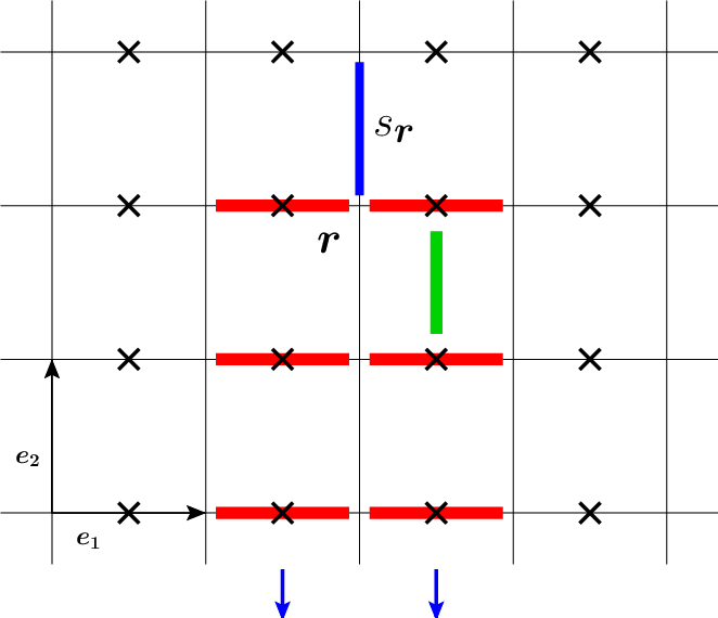
Now, since , Equation (158) shows that satisfies a recurrence relation,
| (159) |
so that
| (160) |
The form of the string operator suggests that we should look for a representation of and in terms of and alone, because then the dual model will feature only half as many degrees of freedom (or equivalently, will act on a state space exponentially smaller). It follows that
| (161) |
and the dual, completely gauge-reduced model reads
| (162) |
It is interesting to notice that describes a bundle of horizontal quantum Ising chains that do not interact with each other. The interactions between chains are carried exclusively by the term that contains all the non-local bonds.
The traditional approach to the duality between the gauge model and the Ising model relies more or less implicitly on the construction we have just described [34], because the Hamiltonian of Equation (162) can be mapped to in terms of dual variables, while cannot (this will be explained in detail in the next section). Let us show how this works. The duality (which is now an ordinary, unitarily implementable duality) between and is established by the Isomorphism
| (163) |
Since is a function of , the relation
| (164) |
follows from the ones just listed. The dual variables that follow from the isomorphism of Equation (163) are
| (165) |
that clearly satisfy the correct Pauli algebra, and are essentially the same as the dual variable used in Reference [34].
3.11.5 Dual variables in gauge-reducing dualities
The bond-algebraic approach to dualities of gauge models is remarkably simpler than the traditional approach [22, 34], and it is also unrelated, because the homomorphism cannot be extended to define dual variables. To see this, suppose to the contrary that we can extend the action of the gauge-reducing homomorphism defined in Equation (146) to include the spins , , so that
| (166) |
becomes a meaningful operation. Then, on one hand, this would imply that
| (167) |
But, on the other hand,
| (168) |
which, together with the previous equation, implies that
| (169) |
Since this is in contradiction with the fact that , we see that we cannot extend the action of to the spins in a consistent way. In other words, cannot be used to define dual spins .
This conclusion seems paradoxical because must be projectively unitarily implementable. Then, it would seem natural to define
| (170) |
Notice, however, that this extension of to operators that are not gauge-invariant is not multiplicative. In other words, the relation
| (171) |
only holds true if and commute with all the gauge symmetries. This means that we should not expect the operator of Equation (170) to satisfy the correct anti-commutation relations with , and also explains the paradoxical conclusion of the last paragraph (), that was derived precisely on the assumption that Equation (171) holds true in general.
The fact that Equation (171) only works for gauge-invariant operators follows from the general relations of Equations (139) and (141). First notice that
| (172) | |||||
| (173) |
(since ). Then, it follows from the decomposition
| (174) |
that
| (175) |
But, if and only if, and commute with all the gauge symmetries, then they also commute with as well, so that we can further write
| (176) |
In summary, is defined on any operator, but it acts as an algebra homomorphism only on gauge-invariant operators.
3.12 Unifying classical and quantum dualities
This section explains one of the most important new results in this paper: a bond-algebraic approach to dualities in classical statistical mechanics [15] (classical dualities described in Section 2.1 and Appendix A). To our knowledge, this section’s results have been completely overlooked in the literature, possibly because the key fact that dualities are unitary or projective unitary mappings [15], has been unclear or overlooked up to now as well. Some advantages of the bond-algebraic over the traditional approach of Appendix A to classical dualities will be discussed in detail in Section 7, but we present here for illustration a toy example, a new self-duality for the classical Ising chain in an external magnetic field. Elementary as it is, this duality is noteworthy because the traditional approach to classical dualities described in Appendix A fails in the presence of a minimally coupled external field, and could not have been used to derive it. The bond-algebraic approach to classical dualities is only rigorously applicable to models that admit a transfer matrix formulation. While this covers a very wide range of interesting models, of finite of infinite size extent, there are dualities for models outside this category, most famously, the duality of the solid-on-solid (SoS) model to a coulomb gas [21]. We explain these dualities in Appendix E.
We associate bond algebras to partition functions of classical models through the transfer matrix. The transfer matrix formalism [5, 28] permits to recast partition functions as traces of linear operators, and can come in several different flavors. For example, row-to-row transfer matrices permit to write
| (177) |
where is an integer related to the number of sites in one of the lattice directions, that one can think of as the Euclidean time direction, and contain information about the directions transverse to the time direction, and how constant-time sections of the lattice are connected from one time to the next. Written as in Equation (177), must satisfy periodic boundary conditions in the time direction. In contrast, corner transfer matrices [28] permit to write
| (178) |
where is fixed, the size of the lattice is completely encoded in the , and the BCs are not fixed by the structure of Equation (178).
This paper will only consider row-to-row transfer matrices, so from now on we focus on Equation (177), keeping in mind though that it is possible to extend our formalism to other types of transfer matrices. The general arguments of Section 3.1 concerning the additive bond structure of physical Hamiltonians can be repeated verbatim for transfer matrices, with the only difference that transfer matrices display a multiplicative rather than additive bond structure:
| (179) |
( stands for a general index). The are now the bonds of interest, and the definition of bond algebra proceeds as before, see Section 3.1.
Suppose next that you have an isomorphic representation of the bond algebra , generated by a set of dual bonds . The dual transfer matrices will define, through Equation (177), a partition function that may look very different from . However,
| (180) |
We call this relation between partition functions, obtained in this way, a classical bond-algebraic duality. Much as with quantum bond-algebraic dualities, we would like to show that:
- •
classical bond-algebraic dualities include traditional classical dualities (at least for models that admit a transfer matrix) [15], and that
- •
classical bond-algebraic dualities are useful.
Both points will be discussed at length in Section 7 where we derive classical dualities, old and new, by bond-algebraic methods. We would like, however, to advance here some support for the second point, by illustrating our ideas with a new self-duality that is elementary, and yet cannot be derived by traditional (Fourier-based) means (Appendix A).
The partition function of the periodic Ising chain of length () is
| (181) |
where
| (182) |
and we assume that . In this case, the row-to-row transfer matrix connects rows that feature one Ising degree of freedom only. The bond algebra of and is symmetric under the exchange (this is just a rotation in spin space). It follows that
| (183) |
provided the dual couplings satisfy
| (184) |
and
| (185) |
Then, Equations (182) and (183) put together define the bond-algebraic classical duality
| (186) |
where we have used the cyclic property of the trace. Notice how linear bond algebraic operations (the exchange ) produce highly non-linear relations between classical couplings. The classical self-dual line determined by and is characterized by
| (187) |
This self-dual line is only critical when and , i.e., at zero temperature.
To our knowledge, the classical self-duality embodied in Equations (186) and (184), valid for any , has not been written before in the literature despite its simplicity. It has, however, one remarkable feature: it is a duality for a model in a minimally-coupled external field, and dualities for such models are beyond the traditional approach as described in Appendix A, and References [30, 31, 6, 7]. The reason is that the standard approach relies on the Fourier transform technique for establishing dualities, and, for these models with two-body interactions, on having individual Boltzmann weights that define circulant matrices [65]. But the Boltzmann weights in cannot be chosen to be circulant except if . Therefore, the self-duality of Equation (186) is not attainable by the Fourier transform method. We think that this indicates that our bond-algebraic approach to classical dualities may push its scope beyond the standard paradigm of Fourier transforms, perhaps even to include classical non-Abelian dualities, though this is a matter under study.
There is a different albeit related way to connect bond-algebraic quantum dualities to classical dualities. It exploits the well-known relation between partition functions of classical problems in dimensions and quantum Hamiltonian problems in dimensions. Quantum mechanical problems in Euclidean time (or equivalently, at finite temperature) can be mapped to a classical partition function problem by use of Feynman’s path integral for the case of quantum particles [56] and fields [57], or by use of the closely related Suzuki-Trotter-Lie (STL) decomposition for quantum lattice models [58, 21]. This quantum-classical mapping takes the general form [21]
| (188) |
where stands for the path integral/partition function, and the classical, , and quantum, , couplings typically connected by non-linear functional relations. In general, this quantum-classical mapping takes quantum problems in dimensions into classical problems in dimensions where the extra dimension, because of the construction, attains periodic BCs [21].
Now we can translate duality properties of into properties of . Suppose that the Hamiltonian is dual to another Hamiltonian as in Equations (95), . Then, with the aid of the identity ,
| (189) |
which implies that
| (190) |
with an analytic proportionality factor that is model specific. Thus, every quantum duality translates into a classical duality [15]. Notice that it is crucial that is a unitary or projective unitary, a fact that was overlooked in the past [15].
Due to the results of Section 3.6, the duality relation (190) can be made exact for any finite size system , and not just for the thermodynamic limit . Rigorously speaking this is always the case, with quantum and classical dualities representing two sides of the same coin. On the other hand, there is a useful practical algorithm, that will be presented in Section 7, that makes use of the STL decomposition and where the thermodynamic limit is, in principle, required [21]. Typically, the use of the STL decomposition implies that the derived classical model presents infinitesimally weak and infinitely-strong couplings, and so the classical dualities derived in this way are less clearly established. It is also important to keep in mind that the classical model of Equation (188) depends on the quantum couplings not just through , in the sense that different quantum couplings can relate to qualitatively very different classical models (and not just the same at different values of ). For example, the STL decomposition maps a single quantum spin to the model of Equation (181) (in the limit , provided ), and not otherwise. Similar constraints apply elsewhere. As dualities relate different regions in the coupling spaces of quantum problems, it is essential to keep track of exactly which classical problems may correspond to a given quantum system for each set of couplings.
4 Quantum self-dualities by example: Lattice models
4.1 Self-dualities in the Potts, vector Potts, and clock models
In this section, we will study two self-dual generalizations of the dimensional quantum Ising chain: the quantum Potts (P) and vector Potts (VP) models (also known as -clock model [21, 29]). These models are just two special examples of a large class of clock models [59], that we discuss too, but very briefly. The fact that the family of clock models contains so many self-dual members is remarkable because clock models have non-Abelian symmetries for . In other words, this section discusses important examples of, inappropriately called, non-Abelian self-dualities (see Section 3.5 for a critical discussion of the notion of non-Abelian duality). To the best of our knowledge, the fact that these models display non-Abelian symmetries has been overlooked up to now.
Potts models feature spins confined to a plain that can exist in any one of different states, and if , they reduce to the Ising model. We know already that in that case, the unitary implementing the self-duality squares to one. But if the self-duality is the square root of a non-trivial discrete symmetry. This illustrates some ideas discussed in Section 3.8. We will first discuss the VP model in detail, since then the self-dual properties of the P and general clock models will easily follow.
4.1.1 The vector Potts model
The VP model is a popular test ground for exotic critical behavior, such as phase transitions without long-range order [60, 61]. The configurations of the classical, VP model are specified by a set of discretized angles
| (191) |
situated at the sites of a square lattice, and its partition function reads
| (192) |
The statistical mechanics of this model has been the subject of research for many years, but there are still open problems. For example, the VP model is known to exhibit a Kosterlitz-Thouless (KT) phase transition [62], for sufficiently large [63], yet to determine the smallest required for a KT transition is a difficult problem, currently under debate [61]. Reference [61] discusses the phase diagram, the nature of the transitions and topological excitations of the VP model, and unveils the U(1) symmetry, that emerges for , associated with the appearance of discrete vortices and KT transitions.
In preparation for writing the quantum model corresponding to the classical VP model by the quantum-classical mapping [21], we introduce some basic facts about the Weyl group algebra [64]. Its generators and are operators characterized by the relations
| (193) |
where is a th root of unity. Equations (193) completely determine the irreducible, finite dimensional, representations of and . A matrix representation is given by
| (194) |
is sometimes called the fundamental circulant (unitary) matrix because it generates the (commutative) algebra of circulant matrices (meaning that any circulant matrix is of the form [65]). and together generate the full algebra of complex matrices, that we continue to call the Weyl group algebra, to emphasize that we are working with a distinguished set of generators.
The Weyl group algebra admits a unitary automorphism in the form of a discrete Fourier transform [64] that, essentially, interchanges the two types of operators ( and their Hermitian conjugates) of the Weyl algebra. A direct calculation reveals that the unitary and symmetric Fourier matrix with maps
| (195) |
With these notations in place, we can proceed to introduce the quantum VP model [66],
| (196) |
(the link to its classical counterpart is worked out Section 7.2), and to study its bond algebra generated by
| (197) |
It is readily verified, either from Equation (193) or Equation (195), that the mapping
| (198) |
(together with the corresponding relations for the Hermitian conjugate bonds) defines a self-duality isomorphism of that maps .
The existence of the self-duality automorphism is intimately connected to (i) the connectivity of the system, as determined by the structure of interactions (specifically, in this case, by the non-commutativity amongst bonds), and (ii) the local degrees of freedom posses a local symmetry which, in this case, is captured by the automorphism of Equation (195). The fact that these two ingredients can be combined consistently renders self-dual. Although not all (self-) dualities follow from this pattern, many do. An interesting exception was presented in Section 3.10.
As explained in Section 3.4, determines the dual variables for the problem. Since can we written in terms of bonds as
| (199) |
the dual variables are
| (200) | |||||
The fact that , satisfy the same algebra as the , affords a useful independent check of the correctness of as a bond algebra isomorphism.
The product of a direct degree of freedom and its neighbor dual satisfy the non-local algebra
| (201) |
This suggests that if , the excitations of the model are governed by the parafermionic statistics that were described in Reference [67] for classical -state models, see the discussion at the end of Section 3.9. For , Equation (201) reduces to the fermionic algebra associated with the Ising model.
Next we show that the group of symmetries of the VP model is non-Abelian for . The first step is to introduce two new operators that act on the basis states of the VP model at site as follows:
| (202) |
The arithmetic in these definitions is modular, modulo . For example, if , then , , and so on. If , and , so we assume in what follows that .
Let us define and . is known in the literature as the charge conjugation operator [68], but, to the best of our knowledge, has not been discussed before. Both and are unitary and Hermitian, see Equation (206) below. Since the operators and act basis states as
| (203) |
it follows from Equation (202) that
| (204) | |||||
| (205) |
Toghether with their Hermitian conjugates, the relations of Equation (204) can be used to show that and commute with . Moreover,
| (206) |
This means [69] that the group of symmetries of the VP model generated by , provides a representation of the non-Abelian polyhedral group . The unitary generates the well-known subgroup of symmetries, since . As it turns out, many models, including the gauge theories discussed in Sections 5.3 and 6.4, have this group among its symmetries.
Our discussion of the VP model presented above has the disadvantage that the dual variables of Equation (200) are not strictly speaking well defined operators (see Section 3.4). We remedy this by considering a finite-size chain with self-dual BCs
| (207) |
The first step in constructing the finite self-duality isomorphism is to match the bonds at the boundaries of the chain
| (208) |
where was defined in Equation (195). Next, we extend the mapping to the remaining bonds,
| (209) |
guided by the fact that we must preserve the connectivity of the interactions and exploit the local symmetry of the Weyl group algebra. In Equation (209), the reflection map of site is defined as in Equation (76) (i.e., ). Notice that the unitary that implements the mapping is not just the discrete Fourier transform . The latter maps into ,
| (210) |
Finally, we use to compute well defined dual variables,
| (211) | |||||
According to the general ideas of Section 3.8, the square of the self-duality unitary commutes with the Hamiltonian. One of the advantages of the bond algebraic approach is that we do not need to compute explicitly to figure out the action of as an operator. Since, by construction, conjugation by amounts to applying twice, it follows from Equations (208) and (209) that
| (212) |
Thus comparing with Equation (204), we see that , where is the charge conjugation symmetry of the VP model as discussed above. Notice also that the self-dual BCs of Equation (207) spoil the symmetry of the (infinite) VP model. We could have used self-dual BCs that preserve both symmetries, in agreement with the techniques of Section 3.6 and Appendix D.
4.1.2 The Potts model and general clock models
The Potts (P) model
| (213) |
in dimensions is yet another -state generalization of the Ising model that, unlike the VP model of the previous section, has a very well understood statistical behavior [70] ( if , and otherwise). The P model has a group of global non-Abelian symmetries (if ), the group of permutations of elements.
The quantum rendition of the P model [71] reads
| (214) |
where denotes the integer part of , that is, the largest integer . It follows that the P and VP model coincide for . But even for arbitrary , since the bonds in are powers of the bonds in , it is not hard to see that the self-duality of the VP model, Equation (198), implies the self-duality of the P model.
The form of the Hamiltonians and suggests introducing a family of models that generalize them and interpolates between them, the clock models. They are defined by the Hamiltonians
| (215) |
with , , arbitrary real coupling constants. The duality properties of some of these models where studied in References [72], and the duality properties of their classical counterparts where studied in Reference [59].
The clock models do not have in general as many symmetries as their special case the P model, but they are all non-Abelian, as the operators of Equation (204) commute with for any value of its couplings. Next we can use our experience with the P and VP models to identify immediately the clock models that are self-dual: The Hamiltonian is self-dual in those regions in coupling space where vanishes if and only if vanishes as well. Clearly, the P and VP model belong to two such regions.
4.2 Dualities in some limits and related approximations
It is standard and useful practice to think of some models as related through a limit of some parameter. The VP model of Equation (192) is a good case in point. It is intuitively reasonable to expect that its behavior must approach that of the XY model as the discrete angle becomes very dense in the limit , and in fact this is know to be the case in many respects [63]. Dualities, however, can show some counter-intuitive behavior with respect to limits. This is the topic of this section, with the VP model as main illustration.
Weyl’s group algebra describes states on a finite, equidistant set of points on a unit circle. If we think of the roots of unity as these points, then and will play the role of position operators, while () acts as a clockwise (counter-clockwise) rotation from any of the roots to one of its neighbors. Following Schwinger [64], one can define position , and momentum Hermitian operators, such that
| (216) |
with eigenvalues , and . In matrix form, , and
| (217) |
with . In the limit, Weyl’s algebra relates to the continuous circle and it can be shown that , and . In this subtle limit, of Equation (196) converges to the quantum version of the classical XY model [21] (up to irrelevant constants)
| (218) |
where . Albeit being the limit of the self-dual VP model limit, is not self-dual, but rather dual to the quantum SoS model (see Section 5.2). It follows that the limit of a sequence of self-dual models needs not be self-dual.
There is a profound difference between compact theories (such as those of variables defined on a circle or the compact fields of electromagnetism) and non-compact theories (e.g., a theory whose fields are defined on a line). An example of the latter which shares some relation to is a linear chain of coupled harmonic oscillators representing acoustic phonons [73]
| (219) |
However, unlike the Hamiltonian is self-dual under the exchange , as the isomorphism
| (220) |
shows. This self-duality arises due an interplay between the connectivity of the model and the automorphism of the Heisenberg algebra
| (221) |
and generates the set of dual variables
| (222) |
The ground state of does not show a phase transition at the self-dual point , or anywhere else for that matter. Thus we see that while self-dualities can constrain phase transitions greatly, they cannot guarantee by themselves that a phase transition will occur.
4.3 The Xu-Moore model
The Xu-Moore (XM) Hamiltonian,
| (223) |
with
| (224) |
was introduced in Reference [74] as an effective model to study ordering in arrays of Josephson-coupled superconducting grains. looks similar to the gauge theory studied Section 3.11, but the fact that the spins are now located at the vertices of a square lattice (see Figure 2) rather than at its links, makes the symmetries and properties of the two models very different. In fact, unlike the gauge theory, the XM model is self-dual [74], and displays dimensional gauge-like symmetries [20],
| (225) |
, that make the model a toy example of topological quantum order and dimensional reduction [20] (see also Section 6.7). Its self-duality is the subject of this section.
The bond algebra generated by the set of bonds is characterized by three relations: Every bond (i) squares to one, (ii) anti-commutes with four other neighboring bonds, and (iii) commutes with every other bond. It follows that there is an isomorphism
| (226) |
illustrated in Figure 10, that establishes the self-duality of the XM model.
As it should, is a symmetry of the model,
| (227) |
but it shows also unsettling features that are typical of working directly in the limit of infinite size. Since formally , it seems that one could argue that is in fact a multivalued mapping,
| (228) |
This is not a problem, however, in the light of the general discussion of Section 3.6.

To make contact with the traditional approach described in Section 2.1 and exploited in Reference [74], we need to employ the ideas of Section 3.4 to compute dual variables. Since
| (229) |
where , it follows that
| (230) |
This completes the calculation.
Let us discuss next self-dual, open BCs for the XM Hamiltonian. Consider an square portion of the infinite model, featuring spins,
| (231) |
(). The goal is to determine boundary corrections to make self-dual, and as usual, this could be accomplished by a systematic study of ’s bond algebra. But this task grows increasingly harder with dimension, so it is important to realize that there is a simple recipe to construct self-dual boundary terms that works well in general (but not always), and that we illustrate next with the XM model. The starting point is the self-duality mapping for the infinitely large model.

So imagine that we try to apply the self-duality isomorphism of Equation (226) to the bonds in . The problem is that, as defined in Equation (231), does not have any plaquettes to which we can map the spins at the left edge and the spins at the top edge (see Figure 11). This suggests that to restore self-duality, we should re-introduce the missing plaquettes as boundary corrections, or maybe incomplete versions of these plaquettes, in order to preserve the number of spins.
As it turns out, this idea works perfectly, so it is convenient to introduce some notation to describe complete and incomplete plaquettes in a unified manner. We write for the plaquette, or incomplete plaquette, that results from simplifying the standard plaquette of Equation (224) by discarding the spins outside the square region encompassed by . So, for example,
| (232) |
Our proposal is that
| (233) |
is a finite self-dual rendition of the XM model ( is illustrated in Figure 11, for ). To prove this, we must construct the self-duality isomorphism, starting by noticing that can only map to . The full isomorphism follows right away,
| (234) |
Geometrically, it is a reflection along the main diagonal, and .
The self-dual BC illustrated in Figure 11 breaks the global , and all the gauge-like [20] symmetries of the XM model, and one could have chosen among several other ones that preserve some or all of these symmetries (see Section 3.6). In particular, if we just replace in Equations (233) and (234) the incomplete plaquettes with standard, complete ones , the resulting model is self-dual under the same mapping, and moreover has all the global and gauge-like symmetries of the XM model. On the other hand, the self-dual BCs that we chose guarantee that all of the spins contained in the square region encompassed by are elements in its bond algebra. Thus we can use the finite isomorphism just defined in Equation (234) to compute finite dual variables. It is convenient to do so, at least for small system size, to check the algebraic consistency of Equation (234). For ,
| (235) | |||||
5 Quantum dualities by example: Lattice models
5.1 XY/solid-on-solid models
The best developed approach to the Kosterlitz-Thouless phase transition of the classical XY model exploits two duality transformations (see for example Reference [21]). First one maps the XY model, via a Villain approximation, to the SoS model, to proceed afterwards to map the SoS model to a classical Coulomb gas. The two steps combined leads to the mapping between the XY model and a Coulomb gas for which deconfinement of charges can be shown to occur at sufficiently high temperatures.
In this section, we will study the first of these dualities to the SoS model from a quantum, bond-algebraic perspective. The SoS model is specified by the partition function
| (236) |
where the classical degrees of freedom reside on the vertices of a square lattice (see Figure 2).
The quantum version of the SoS model must have states labelled by integers . Three operators are then required to describe its quantum dynamics: a position operator , and left/right shift operators ,
| (237) |
that satisfy
| (238) |
and generate an algebra isomorphic to the one satisfied by the elementary degree of freedom associated to Equation (218), . In particular, and have identical spectra.
The duality mapping between the quantum versions of the XY and the SoS models can be derived by comparing the bond algebra generated by
| (239) |
which is characterized by the relations
| (240) |
and the one generated by the SoS operators
| (241) |
Then, the isomorphism
| (242) |
establishes a duality between the two models (a related mapping in terms of less well-defined operators was described in Reference [75]). The dual form of reads
| (243) |
which to our knowledge has not been reported in the literature before. One can verify, using the standard quantum-classical mapping [21], that the classical counterpart of is indeed the classical SoS model of Equation (236).
This duality is similar, in spirit, to the self-duality of the quantum Ising chain as seen through the dual variables
| (244) |
The inverse of the isomorphism of Equation (242) defines a reciprocal set of dual variables.
5.2 Xu-Moore/planar orbital compass models
The planar orbital compass (POC) model of orbital ordering [76],
| (245) |
features spins residing on the vertices of a square lattice (see Figure 2), and interacting in such a way that strongly correlates directions in real and spin space. The POC model is dual to the XM model studied in Section 4.2 [77] (for another duality see [78]), as follows from the duality isomorphism
| (246) |
so that . If follows that the POC model is self-dual.
The inverse duality transformation reads
| (247) |
and both and define their own set of variables. From Equation (246),
so that ( means the Hamiltonian written in term of the variables inside the brackets). Similarly, from Equation (247),
| (248) | |||||
so that .

Boundary corrections are required to preserve the duality for finite lattices. One possible set of boundary terms is shown in Figure 12, for a lattice. Both models, including the boundary corrections, have now nine -like and nine -like bonds. The duality isomorphism is given below,
| (249) |
In Equation (249), the bonds to the left of the double arrow are those of the XM model and those to the right denote bonds of the orbital compass model. Albeit being tedious, it is straightforward to extend Equation (249) to an square lattice. This explicit transformation enables the computation of all dual variables.
5.3 Two-dimensional gauge/vector Potts models
In this section we study a gauge-reducing duality, along the lines of Section 3.11.
The dimensional gauge theory [33],
| (250) |
with
| (251) |
is a generalization of the Ising gauge model studied in Section 3.11, Equation (143). The operators (), located at the links (see Figure 2) of a square lattice, commute on different links, and satisfy the algebra described in Section 4.1.1 otherwise. As the name of the model suggests, displays a gauge symmetry as realized by the local symmetry operators
| (252) |
However, the global symmetries of the model are non-Abelian, as can be seen by folowing the discussion in Section 4.1.1 of the symmetries of the VP model.
We want to find a transformation to a dual Hamiltonian which is free of gauge symmetries. The dimensional quantum VP model (a higher-dimensional version of Equation (196))
| (253) |
is a natural candidate, because it is a generalization of the Ising model in a transverse field in terms of Weyl group algebra operators (defined on the vertices of the lattice, see Figure 2). It is not hard to find a bond algebra homomorphism that confirms the duality,
| (254) |
up to the complete elimination of gauge symmetries,
| (255) |
5.4 Two-dimensional compact QED and XY models
The elimination of gauge symmetries has a slightly different flavor for models that feature continuous (or merely infinite) degrees of freedom, essentially because it becomes more convenient to work with the Hermitian generators of the gauge symmetries, rather than with the unitary symmetries themselves. This section presents two examples of this kind, a gauge-reducing duality for compact QED to the SoS model, and a duality from a gauge SoS model to the XY model. These quantum dualities are new to the best of our knowledge, but a classical () relative (performed by way of the Villain approximation) of the duality for the XY model was first used in Reference [79].
The Hamiltonian for compact QED that follows from Wilson’s lattice QED [80] can be worked out along the lines of Reference [81],
| (256) |
It features continuous angular variables defined on the links of a square lattice, with
| (257) |
and where the elementary degrees of freedom satisfy the operator algebra
| (258) |
The gauge symmetries of Wilson’s action translates in the Hamiltonian language to the fact that commutes with all the star operators
| (259) |
These are the infinitesimal generators of gauge symmetries.
The gauge-reducing duality that we describe next is a hybrid between the dualities presented in Sections 5.1 and 5.3. It allow us to recast the gauge invariant information contained in in a form that is free of gauge redundancies. The dual, completely gauge reduced model is the SoS model
| (260) |
that features elementary degrees of freedom placed on the sites of a square lattice, and can be connected to the classical SoS model through a STL decomposition (see Section 3.12). The operators at site satisfy the relations of Equation (238), and commute with the operators on other sites. Notice that possesses global symmetries only.
The connection between and is established through the homomorphism of bond algebras
| (261) | |||||
That the gauge symmetries of are trivialized (eliminated) by the duality follows from the computation
| (262) | |||||
Next we consider a duality that is in some sense complementary to the previous one. The XY model
| (263) |
is the completely gauge-reduced version of a gauge SoS model,
| (264) |
where . The generators of the group of gauge symmetries of are
| (265) |
but these are not infinitesimal. The gauge-reducing duality to the XY model is established by the homomorphism of bond algebras
| (266) | |||
that satisfies
| (267) |
5.5 Toric code/ Higgs models
Over the last fifteen years quantum computation has become a well developed theoretical discipline, fostering a paradigm-breaking new understanding of computational complexity and quantum mechanics [82]. In contrast, the technological problem of building a quantum computer remains essentially unsolved, and one of the biggest challenges is the realization of quantum memories.
Kitaev’s toric code (TC) model [83] (see Equation (275)) is an excellent example of the virtues and pitfalls of one of the most popular approaches to the problem of storing quantum information: the use of topological quantum order [20]. While the TC model is a good example of topological quantum order, it fails as a quantum memory at any finite temperature [20]. This surprising result, known as thermal fragility [20, 84], could be proved and probed in detail thanks to the realization [20] that the TC model is (exactly) dual to two decoupled Ising chains in zero magnetic field, a duality established by arguments that are direct precursors of the bond-algebraic machinery.
Whether or not topological quantum order turns out to be key to the implementation of quantum memories or the quantum computer, it is clear by now that, as an order of matter that goes beyond the Landau symmetry-breakdown paradigm, it is worth studying in its own right. In this section we show that two popular models to study topological quantum order, the extended toric code (ETC) model in two [85] and three space dimensions, are dual to the Higgs model [86]. While the duality in dimensions is already exploited in Reference [85] to help the numerical simulation of the ETC model, the duality in dimensions is one of the most interesting new dualities reported in this paper. Both dualities are in fact special cases of a general gauge-reducing duality for the Higgs model that works in any number of space dimensions, and that is also special in that it does not necessitates the introduction of non-local string operators (recall the discussion of Section 3.11.4). Other aspects of this duality will be discussed in Section 6.4. Section 8.5 presents a broader discussion of the role of dualities in the study of topological quantum order.
The Higgs model in spatial dimensions
| (268) |
features spin degrees of freedom on the sites and links of a hyper-cubic lattice. It can be thought of as a lattice, two-state approximation to a complex Higgs field of fixed modulus (or in its broken symmetry phase [6]), in interaction with electromagnetism, and it represents one of the best understood models of confinement in dimensions and . Its gauge symmetries are
| (269) |
The goal of this section is to find a completely gauge-reducing duality to take care of this gauge redundancy.
The structure of s bond algebra suggests the model
| (270) |
for a gauge-reduced dual. shows no local symmetries, due to the couplings to external magnetic fields, and the bond algebra homomorphism that connects it to follows naturally,
| (271) |
To check that is indeed gauge reducing, we compute
| (272) |
Notice that the completely gauge-reduced model features only degrees of freedom on the links of the lattice, and local bonds.
The duality just described works in any space dimension . In , the models have well known physical meanings. The Higgs model
| (273) |
is dual to
| (274) |
which is just an Ising chain in the presence of transverse and longitudinal fields [86]. This means that has no phase transition when . We see that the gauge field has opened a mass gap in the model.
In dimensions, the gauge reduced form of the Higgs model reads
| (275) |
( was defined in Equation (60)). This is exactly the ETC model of Reference [85] (if we further set , we recover Kitaev’s TC model). The duality maps the Coulomb phase [86] of the Higgs model to the topological quantum ordered state of the ETC model.
In dimensions, the Higgs model is self-dual [32], which implies that the ETC model is self-dual as well [85, 15]. Let us check this in the latter model. The self-duality isomorphism [15] reads
| (276) |
that exchanges with , and simultaneously with in . This is one of the rare instances where a self-duality mapping is local in the spins. Other interesting dualities for the ETC model are reported in [15] (and its supplemental material).
The gauge-reduced version of is again intimately connected to a dimensional generalization of the ETC model
| (277) | |||||
studied in Reference [84] in the case of vanishing magnetic fields. The phase diagram of the full model, that we call the ETC model, can be obtained from the literature on the Higgs model (see, for example, Reference [86], Figure 2).
6 Bond-algebraic dualities in quantum field theory
Over the years, some of the most interesting and ambitious dualities have been conjectured in the context of quantum field theory (QFT) [87, 11], and any progress in the theory of non-Abelian dualities should be tested against QCD (quantum chromodynamics). The functional approach to QFT [57] puts QFTs in a language that resembles closely that of classical statistical mechanics. Therefore there have been some attempts [88] at dualities for path integrals of QFTs that resemble that of Kramers and Wannier introduced in Section 2.1. However, the progress in this direction has been limited (see though References [89, 90, 91]). The situation improves considerably if the (Euclidean) path integral for the QFT of interest is regularized by replacing the continuum for a lattice [80] (see Appendix C). Then, for Abelian theories, one can use the machinery of Appendix A to construct systematically regularized dual (Euclidean) field theories [6]. But, as discussed in Section 3.12, and illustrated in Section 7, this path-integral based, lattice approach to dualities in QFT is covered, and in fact simplified by the bond-algebraic techniques of this paper [15]. In this light, many of the dualities we have seen already can be interpreted as bond-algebraic dualities for QFTs.
In contrast, this section aims to explore the extension of bond algebraic techniques to operator-based quantizations of field theories. This is perfectly feasible for some QFTs, but in general we do not know yet how to construct a complete operator quantization of an interacting field theory, and so in many cases the bond algebra of an interacting QFT is not well defined. This means for instance that we could have trouble deciding whether two operators in a QFT should commute or not, as exemplified by the Schwinger term in QED [92]: The canonical quantization of electromagnetism in interaction with the Dirac electron field dictates the charge density operator should commute with the current, but in fact this is inconsistent with the requirement that the theory should have a ground state [92]. It follows that this commutation relation must be changed relative to its canonical form.
There is an approximate approach to the operator quantization of field theories that is specially compatible with bond-algebraic techniques, and was popularized in the literature on confinement under the name of lattice Hamiltonian formalism [81, 34]. The idea is to discretize the classical field theory first only in space (that is, to approximate it with a classical mechanical model featuring degrees of freedom on a spatial lattice), and then proceed to quantization, that can now be carried through by standard means (see Appendix C). The resulting many-body quantum theory typically features non-relativistic bosons, fermions, or rigid rotators in interaction, and contains a new parameter, the lattice spacing . Of course, it lacks the symmetries characteristic of the continuum, but has in exchange a well defined operator content, and typically internal and gauge symmetries are well represented. In what follows, we study the duality properties of several QFTs in this approximation. But when possible, we work also directly in the continuum, and show that the two approaches give compatible results when a naive continuum limit is taken.
6.1 One-dimensional free and externally coupled bosonic field, and the Kibble model
The free, massless bosonic field in (i.e., 1+1 space-time dimensions) affords the simplest example of a self-dual QFT [1, 15]. In dimensions , a complete operator quantization is always available for free fields [93]. This is not the case in dimension . In particular, the Green’s function for the massless boson field is too singular to be interpreted in the sense of distributions. Still, its bond-algebra based on canonical quantization reflects its self-dual properties, and we can check them in the lattice Hamiltonian approximation. In this approximation, the bosonic field reduces to a self-dual model of one dimensional phonons, Section 4.2, and the phononic lattice dual variables converge to the bosonic dual variables in the continuum. Next we consider two simple extensions, the Kibble model in Section 6.1.2, and a multiplet of bosonic fields in interaction with an external driving forces.
6.1.1 Free, Massless bosonic field
The massless, free bosonic field in dimensions, () is described by the action
| (278) |
where , stands for the time coordinate, and for the spatial coordinate. Its canonical quantization proceeds by defining the Hamiltonian
| (279) |
together with the equal-time commutation relations
| (280) |
One may think of as the quantum theory of a continuous elastic line (see Reference [73], Chapter 2).
From the perspective of bond algebras, the new feature is that we have an uncountable infinity of bonds, two bonds per space point. It is easier to characterize the bond algebra in terms of and ,
| (281) |
where is the spatial derivative of the Dirac delta function. It is apparent from this relation that
| (282) |
is a self-duality isomorphism, since
| (283) |
and .
Next we use Equation (282) to compute dual variables. Since
| (284) |
the dual field variables are
| (285) | |||||
We may regard these dual fields as toy examples of Mandelstam variables [94], the variables that appear in the bosonization of theories [95].
Let us compare next the calculations in the continuum to the predictions of the lattice Hamiltonian approach. If we discretize in space the action of Equation (278), and quantize afterwards, we get a quantum model specified by
| (286) |
with the lattice spacing. This model is essentially identical to the self-dual model of phonons studied in Section 4.2, and thus self-dual as well (notice that while is dimensionless, has dimensions of ). Its self-duality mapping can be read from Equation (220),
| (287) |
and it clearly converges to the corresponding mapping in the continuum, Equation (282), in the naive continuum limit .
6.1.2 The one-dimensional Kibble model
The self-duality mapping investigated in the previous section is readily applicable to the Kibble model [96],
| (288) |
in dimension. The version of this model with Coulomb potential has been studied as an example of a model that violates Goldstone theorem [21], due to the long-range nature of the Coulomb interaction.
The Kibble model has the unusual feature that the momenta participate in the interaction term. In this is remedied by the duality of the previous section. The mapping of Equation (282) shows that admits a dual representation
| (289) |
so that now the interaction term involves only spatial gradients.
6.1.3 Massless bosonic field coupled to classical external sources
The self-duality of the free boson field survives even after we have coupled it to classical, external sources and ,
| (290) |
that vanish outside some finite interval. While the coupling is standard, the coupling is not, because is not the vector potential for an EM field (for one thing, is not charged). We introduce it anyways, because the self-duality we are going to describe exchanges and .
The next step is to apply to the self-duality mapping for the free boson field, Equation (285). After some rearrangements (that include discarding a boundary term, since has compact support), the resulting Hamiltonian reads
| (291) |
with
| (292) |
Since has the same structure as (up to an additive c-number), we see that is still self-dual as in the free case. Notice that , since and .
6.2 The Luttinger model
Next we describe a duality for fermions in one dimension. The Luttinger model describes a dimensional interacting many-electron system in a box of size . Its Fermi surface consists of only two points, , corresponding to two types of electrons moving to the right/left. Henceforth, we denote the right and left moving electrons by the fields and (which anti-commute) and construct a two component field . In the vicinity of the two Fermi points (i.e., for small and small for or small for ), the free electron dispersion may be linearised to read with the Fermi velocity. The (spinless) Luttinger model is defined by the Hamiltonian
| (293) |
In Equation (293), the first term describes the free electron dispersion (with set to unity). This is augmented, in the second term of Equation (293), by density-density interactions that couple left () and right () movers. By explicitly constructing unitary transformations, Luttinger showed that is unitarily equivalent to a non-interacting model, and thus it is exactly solvable (see, for example, [97] and references therein). It has, however, the non-physical characteristic that in the thermodynamic limit it displays an infinite reservoir of negative energy states.
We will next re-derive this unitary equivalence within the bond algebraic framework. The Hamiltonian commutes with particle number operators for each fermion species (left and right movers), and can be written in a first-quantized form as
| (294) |
where and are the momenta and positions associated with the right (a total of ) and left (a total of ) movers. The wave functions on which operates must be totally antisymmetric because of Fermi statistics. Luttinger’s result amounts to the statement that is dual to
| (295) |
To prove this result from a bond-algebraic perspective, we introduce the bonds
| (296) |
so that
| (297) |
It is immediate that
| (298) |
since
| (299) |
Thus, putting all the pieces together, we establish the duality isomorphism
| (300) |
The above demonstration illustrates that Luttinger’s assertion holds for arbitrary interactions in Equation (293).
6.3 QED without sources, compact QED, and gauge theories
6.3.1 QED without sources
The quantization of the EM field suffers from well known complications due to gauge invariance, and very different from the complications that arise in the quantization of the free boson. They are much less of a problem from a bond algebraic perspective, because in the end, at least in the absence of sources, we do know how to construct a full operator quantization of the EM field. The resulting vacuum QED is the starting point to quantum optics [98], and is self-dual under the exchange of the quantum electric and magnetic field operators.
We start by setting up the version of QED that we are going to work with. The starting point is the gauge-invariant action for the vector potential,
| (301) |
(the connection of the vector potential to the electric and magnetic fields was described in Section 2.1). To proceed with canonical quantization, we need to partially fix the gauge. If we choose the condition , called the axial gauge, we can complete the canonical quantization prescription easily. The resulting QFT reads
| (302) |
together with
| (303) |
and the can be realized as well defined operators (i.e., operator-valued distributions) action on a Hilbert state space. Notice that in the axial gauge we are using, . There is, however, and issue left from the remaining gauge symmetry of the theory defined by Equations (302) and (303). The state space is larger-than-physical, and only the states that satisfy the Gauss constraint
| (304) |
can be prepared and observed by experimental means. The reason is that is the generator of the residual gauge symmetries that where not fixed by the axial condition , and so Equation (304) amounts to the statement that only gauge invariant states are physical.
Let us consider next the bond algebra characterized by
| (305) |
It is easy to check that the mapping
| (306) |
preserves the relations of Equation (305), but there is a subtlety of interpretation. maps , that is automatically divergenceless, to , that is not. However, is divergenceless in the gauge invariant subspace of physical states, and so is a true isomorphism of bond algebras in that subspace. In the language of Section 3.10, and for this particular quantization of the EM field, its self-duality is an emergent one. In other words, the EM duality is truly a duality between the observable physical electric and magnetic fields, and not a more general property of the vector potential.
We can use the mapping of Equation (306) to compute dual variables on the subspace of physical states,
| (307) |
This completes our discussion of the self-duality of QED in the continuum. The next step is to check it against the lattice Hamiltonian formalism. This analysis will facilitate later our discussions of duality in other Hamiltonian lattice gauge field theories that are closely connected to QED and to the dynamics of center vortices in QCD [22, 33].

If we discretize the EM field as we discretized the free boson field near the end of Section 6.1.1, we get
| (308) |
where , and stands for the discretized curl,
| (309) | |||||
(see Figure 13). The fact that the theory in the continuum features a vector field is reflected in that the lattice degrees of freedom reside on links, with commutation relations
| (310) |
Discretizing the theory spoils its space-time symmetries, but gauge symmetries remain almost unchanged. The generators of gauge symmetries are
| (311) |
and physical states are characterized as before as .

is self-dual, just as its counterpart in the continuum. The mapping
| (312) |
defines a self-duality isomorphism in the subspace of physical states, that exchanges the lattice electric and magnetic operators, see Figures 14 and 15. is not well defined outside the subspace of physical states, because as it stands in Equation (312), it can be shown to be a many-valued mapping, . It is easy to check that the lattice self-duality converges exactly to its counterpart in the continuum in the naive limit .

It is remarkable that, in the end, the EM duality has the same origin as the self-duality of the Ising model: a symmetry of a bond algebra.
6.3.2 Compact QED and gauge theories
The self-dual lattice rendition of QED that we studied in the previous section is non-standard. In contrast, the standard Hamiltonian lattice field theory for QED [34, 81] (see, for example, Section 6 of [34]),
| (313) |
arises from the quantization [34] of compact (lattice) QED as defined by Wilson [80]. Here, the plaquette term is formally defined as in Equation (309) up to the replacement , and the latter satisfy the commutation relations of Equation (258).
The Hamiltonians and exhibit radically different phase diagrams, simply because describes a system of harmonic oscillators, while features plane rotors in interaction. In particular, is not self-dual. On the other hand, one can use the techniques of Sections 4.2 and 5.4 to set up a dual gauge model in terms of integer valued degrees of freedom,
| (314) |
(the plaquette term is formally defined as in Equation (309) up to the replacement , the operators where introduced in Section 4.2). A close classical relative of this duality to integer valued fields was found of great use in the latest comprehensive Monte-Carlo simulation of [99].
We can also use the mathematics introduced in Sections 4.1 and 4.2 to write down a self-dual -state approximation to
| (315) |
that features generators and of Weyl’s group at each link, and
| (316) | |||||
The self-duality mapping for this model was discussed in Reference [15], and is given by
| (317) | |||||
(and similarly for Hermitian conjugate bonds). Similar to the VP model of Section 4.1, the squared duality isomorphism is a non-trivial, discrete charge conjugation symmetry of the model, that maps and to and , up to a translation by . When , the phase structure of approaches that of [100], even though is not self-dual (see Section 4.2).
In this section, we introduced in connection to QED. Actually this model has been intensively studied in the literature [101, 102, 33] in connection to confinement in QCD. This is so as for states affords a simple effective theory to study center vortices in QCD with flavors. This was discussed, to some extent, by ’t Hooft [103] where the relevance of center vortices to confinement was first elucidated, but the specific Hamiltonian was proposed in Reference [33]. From this point of view, however, this lattice model suffers from its inability to incorporate magnetic monopoles. Other aspects of will be discussed in Section 7.4.2.
6.4 QED without a vector potential
In classical physics, the EM vector potential is a technical advantage, but otherwise expendable, essentially because the interaction of classical charged particles with the EM field can be described purely in terms of and . In contrast, the vector potential is unavoidable at the quantum level, and the best illustrations of this fact is the Aharonov-Bohm effect [104] that is non-local in and . But even disregarding the interaction to charges, it is difficult to set up the quantum mechanics of the EM field alone without introducing a vector potential, though Mandelstam [105] managed to put forward a consistent scheme. The standard quantizations of the EM field, however, rely on the unobservable , and suffer from well-known difficulties [106], that depend on the gauge fixing condition of choice. In the axial gauge of the previous section, the state space that emerges is a Hilbert space, but it is redundant, due to the presence of gauge symmetries inherited upon quantization.
On the other hand, as explained in Section 3.11, we can use bond-algebraic dualities to find a dual representation that features no gauge redundancies. In this section, we illustrate these ideas for compact QED, because it is the model of greatest relevance in numerical studies of QED.
Ideally, we would like to find a gauge reducing duality for the Hamiltonian of Equation (313) to a model that features local bonds. We saw in Section 5.4 that this is possible in , but it does not seem to be possible in . Hence we are left with the systematic approach of Section 3.11.4, that is known to introduce non-local bonds in the dual model. The starting point is to recognize the generators of gauge symmetries, in this case
| (318) |
Now we can proceed with the general techniques described in Section 3.11.4. The gauge-reducing duality should satisfy
| (319) |
so that in the completely gauge-reduced dual the bonds are not independent, but we can write instead . From this point on, the reasoning follows through just as in Section 3.11.4. The gauge-reducing duality homomorphism reads
| (320) | |||
(the plaquette angle was defined right after Equation (313)). The electric string operator is defined as
| (321) |
and carries the full weight of the non-locality that seems to be unavoidable in , if gauge constraints are to be eliminated. The completely gauge-reduced dual Hamiltonian reads
| (322) | |||
It is remarkable that describes a stalk of non-interacting (independent) , XY models. The idea that the physics of gauge fields in is closely connected to the physics of spin models in has been put forward many times over the years (see [22], and references therein). The duality just presented is a new indication/realization of this connection. Moreover, it afford us a theory of QED without a vector potential, and consequently, without gauge symmetries or unwanted non-physical states. Stated differently, is the quantum rendition of Maxwell’s dynamics purely in terms of the electric and magnetic fields. The cost to be paid is the introduction of non-local bonds.
From a practical point of view, it is important to notice that this gauge-reducing duality can be restricted to finite systems, and the advantage for numerical simulations of the gauge reduced rendition of the theory could be enormous. For one thing, since there are no degrees of freedom associated with the links along the direction, the Hilbert space of reduces to
| (323) |
that is much smaller than the one for ( denotes the Hilbert space of square integrable functions on the circle). Physically speaking, exhibits two “states of polarization” per lattice site.
6.5 Abelian and Higgs models
In this section we study the duality properties of the Abelian Higgs (AH) QFT in its broken symmetry state. The AH model is complex enough that an operator treatment in the continuum is not well defined, so we proceed directly to the lattice Hamiltonian formalism. We uncover a new duality in to a local, completely gauge-reduced model, introduce new -state approximations to the lattice AH model that we call Higgs models, and discuss their (self-)dual properties in and (the case [22] is of importance to the theory of topological quantum order and storage of quantum information, see Section 5.5). We start with some general comments to put the AH model in perspective.
Both in condensed matter and high energy physics, the success of QFTs in describing interactions hinges to a large extent on the principle of gauge invariance and the Higgs mechanism. The reason for the latter is that, if the gauge group is compact, gauge invariance requires gauge fields to be massless, restricting in principle their applicability to the description of long-range interactions. The Higgs mechanism affords a way out of this restriction, since it is a process by which gauge fields acquire mass through the spontaneous breakdown of a continuous symmetry with no Goldstone bosons. In this way, gauge fields become capable of describing short-range interactions as well, at the expense of introducing a Higgs field.
The AH model,
| (324) |
features a complex scalar Higgs field of charge , in interaction with the EM field ( is the EM field, and ), and it is the simplest field theory that combines both the principle of gauge invariance and the Higgs mechanism. When is positive, the (classical) potential energy is minimized by setting , and the ground state breaks (spontaneously) the symmetry. The reader familiar with superconductivity will recognize the resulting action as the starting point for the phenomenological Ginzburg-Landau theory of superconductivity (wherein represents the superconducting order parameter). In the light of QFT, however, the spontaneous breakdown translates into a particle spectrum containing one massive photon and one massive, real scalar (see, for instance, [106]). This is the Higgs mechanism of mass generation: the would be Goldstone boson associated to the spontaneous symmetry breakdown is reabsorbed as an extra degree of freedom of the gauge field . It is the mechanism of mass generation in the standard model of particle physics, but it is not the only possible one, as we will see in the next section when we study the Stückelberg model.
The lattice Hamiltonian for the AH model in its broken symmetry phase reads
| (325) |
with the notation of Section 6.4 for and . The Higgs, or matter, field is represented by degrees of freedom and on the sites of a cubic lattice, while the gauge field is represented by degrees of freedom , on its links. follows from the classical lattice action introduced in Reference [86], treated according to the quantization techniques of Reference [81]. Notice that is now constrained to take integer values. As discussed in Reference [86], the physics (phase diagram) of the AH model depends strongly upon whether or has some other value, and in fact is an explicit parameter in the duality mappings to be discussed.
defines a gauge theory, with gauge symmetries generated by
| (326) |
It is a remarkable feature that these gauge symmetries are completely eliminated by a duality to a local model,
| (327) |
that features integer-valued degrees of freedom and local bonds. The plaquette operators are defined just as in (316), up to the replacement , and (the operators , and were introduced in Section 5.1). It follows that does not feature any degrees of freedom on the sites of the lattice. The duality homomorphism reads
| (328) |
and it is straightforward to check the trivialization of the infinitesimal generators of gauge symmetries,
| (329) |
has no local symmetries. Let us point out without elaborating the details that the AH model admits a local gauge-reducing duality along these lines in any dimension .
We can take a different approach to the study of the AH model, and write -state approximations to the Hamiltonian of Equation (325), in terms of generators of the Weyl group algebra introduced in Sections 4.1 (this is similar in spirit to the approximation of the XY model by a VP model). We call these -state quantum models Higgs models, and to our knowledge they have not been studied before, for (the case [86, 32, 107] was discussed in Section 5.5 from the perspective of topological quantum order). The Higgs models admit completely gauge-reducing dualities, and the dual models that arise are natural generalizations of the ETC model of Section 5.5, to any number of states and any number of dimensions . Moreover, in , they define a new class of self-dual models. Let us focus on this case for the rest of the section.
The Hamiltonian for the -dimensional Higgs model reads
| (330) | |||||
with gauge symmetries
| (331) |
and . As usual, denote site (vertex) operators, and reside at the link . Notice also that the charge is a charge now, and can only take one of the values . The self-duality mapping reads
| (332) | |||||
Strictly speaking, is an isomorphism only on the restriction of the bond algebra to the subspace of gauge-invariant states, so this is another example of an emergent self-duality (we encountered a similar situation in QED, Section 6.3). To see this, notice that one can expand the identity operator as a product of bonds in many different ways, and that all these different expansions are mapped to products of gauge symmetries. It follows that is a multivalued homomorphism, unless it is restricted to the subspace of gauge-invariant states.
Since features both matter and gauge fields in interaction, it is interesting to compare the self-duality of Equation (332) to the self-duality properties expected of QED in the presence of suitable sources. In general, it is argued that by introducing magnetic charges, the self-duality of QED in the absence of sources, Section 6.3, could be extended to include sources as well. This putative self-duality, however, would not mix matter fields with gauge fields. In contrast, in the Higgs case, the self-duality establishes an equivalence between matter and gauge fields.
The -state models can be completely gauge-reduced by dualities that are very similar to that for , worked out in Section 5.5. There is also a variation of the Higgs models where the VP-like interactions are replaced by P-like interactions [108]. This Potts-Higgs model has the advantage that its phase diagram can be studied analytically in a expansion.
6.6 The self-dual Stückelberg model
In this section we discuss the Stückelberg model of mass generation, and show that it is self-dual in dimensions.
The massless free boson of Section 6.1
| (333) |
(now in any dimension ) has a global, internal continuous symmetry of the form , , but this fact is rarely of interest because the conservation law that follows is tantamount to the equation of motion. Things become more interesting if apply the gauge principle to this symmetry, and gauge it to make it local, at the expense of introducing a vector potential ,
| (334) |
This is the Stückelberg model of mass generation (see [106], and references therein), proposed by Stückelberg in 1958. The gauge symmetries of are
| (335) |
and show that both the and field are not observable. Combined, however, they describe in a gauge invariant fashion a massive vector field (a Proca field) of bare mass (to see this, just impose the gauge-fixing condition in Equation (334)). Since the Proca field can be completely quantized in operator form [93], we expect that the same holds for , and we work directly in the continuum. Still, let us point out that analogous calculations in the lattice Hamiltonian approach return results that are perfectly compatible with the continuum, in the naive continuum limit .
The Stückelberg model is self-dual only in , as will become clear soon, so from now on we work out just that case. The canonical quantization of has the usual complications coming from gauge-invariance. The simplest way to proceed is to partially fix the gauge by imposing the axial constraint . This allows to put in canonical form, so that we can apply the standard quantization procedures to get
| (336) | |||
with , and every other commutator set equal to zero. The subspace of physical, gauge-invariant states is characterized by
| (337) |
That is self-dual follows from the mapping
| (338) | |||||
Since we can write (among other possibilities), we have that
| (339) |
This means that just as in QED, Section 6.3.1, represents a self-duality isomorphism only in the sector of gauge-invariant states, and is multi-valued in the full, gauge-redundant state space.
This completes our discussion of the Stückelberg model, but let us point out in closing that all of the previous results follows just as easily in the lattice Hamiltonian approach.
6.7 Field theory and dimensional reduction
There is an intimate connection between -dimensional systems possessing -dimensional gauge-like symmetries [20], and the phenomenon of dimensional reduction, where the physical system in dimensions behaves in many ways as if it had effectively a smaller number of dimensions [20, 84]. Mathematically, this connection results from establishing bounds for the correlation functions of the -dimensional theory in terms of another theory in dimensions. A very broad and exciting field where dimensional reductions, -dimensional gauge-like symmetries, and dualities come to the fore is that of topological quantum order [20, 84]. In topologically ordered systems, the state of the system cannot be characterized by local measurements but rather by topological quantities.
In this paper, we have considered the duality properties of several lattice models that display topological quantum order, including the XM and POC models of Sections 4.3 and 5.2 [20], and the paradigmatic ETC model of Section 5.5. Here we develop continuum (field-theoretic) versions of those lattice models, where dimensional reduction occurs because of the existence of -dimensional gauge-like symmetries. Consider then the non-relativistic, -dimensional QFT
| (340) |
By construction, this model is invariant under the gauge-like symmetry , where are smooth, real functions of one variable. Also, it is self-dual, as follows from the mapping
| (341) |
that defines the dual variables of the problem. Notice that formally, . This is the standard manifestation (seen many times in formally infinite lattice models, see the discussion in Section 3.6) of the fact that to make rigorous we need to specify self-dual BCs.
In what follows we are going to study these results in some detail on the lattice, to showcase the connection of the model of Equation (340) to other lattice models with gauge-like symmetries. The lattice Hamiltonian approach applied to Equation (340) returns
| (342) |
with , that is self-dual by virtue of
| (343) |
The structure of suggests setting up a -state model of the form
| (344) |
with (the and operators where introduced in Section 4.3). For , defines a class of self-dual models that has not been studied before to the best of our knowledge. For , becomes identical to , the XM model of Section 4.3. The connection between , , and stands on their common self-dual structure and the shared presence of gauge-like symmetries (see Section 4.3 for a discussion of the gauge-like symmetries of the XM model). Thus these models afford an excellent scenario to study the role of dimensional reduction and topological quantum order in more general settings, where the structure of the elementary degrees of freedom are varied in a controlled fashion.
Since shares some formal similarities with the XM model, we expect it to show a duality to a model analogous to the POC model of Section 5.1. The dual model turns out to be
| (345) |
as follows from the mapping
| (346) |
Interestingly, it is easy to take the naive continuum limit of ,
| (347) |
That is indeed dual to the QFT defined in Equation (340) follows from the isomorphism
| (348) |
7 Bond-algebraic approach to classical dualities
In this section we establish dualities for models of classical statistical mechanics, exploiting the theory of Section 3.12, and introduce a new classical gauge model that is self-dual for any . The aim is to illustrate the unification of the theory of dualities in the framework of bond algebras, and the advantages of approaching classical dualities from this new perspective. On the other hand, it is important to keep in sight the related fact that quantum dualities are fundamentally related to classical ones by path integrals or the the STL decomposition (see Section 3.12). These widely used techniques approximates the exponential of a sum of (non-commuting) operators by products of exponentials
| (349) |
with an error assumed to be bounded [56], and, combined with bond-algebraic techniques, they can afford a simple fast way to connect quantum dualities to classical dualities [15, 21]. In the following, however, we will bypass the use of the STL decomposition technique, to obtain exact duality mappings between finite or infinite models of classical statistical physics.
7.1 The classical Ising model in the Utiyama lattice
As mentioned in Section 2.1, one of the most celebrated self-dualities discovered long ago by Kramers and Wannier enabled a quantitative prediction [4] of the critical temperature of the classical Ising model in a square lattice. From a bond-algebraic perspective this self duality is a consequence of the self-duality of the quantum Ising chain of Section 3.6. Since this calculation is already available in textbook form [21], we present in this section the most general case of a duality for the classical Ising model in the Utiyama lattice [109] defined in Figure 16.
The partition function that describes Utiyama’s anisotropic, bipartite classical Ising model
| (350) | |||
features four different nearest-neighbor couplings, , arranged as shown in Figure 16 (a point is even if , and odd otherwise). The advantage in studying is that it describes in a unified fashion several important renditions of the Ising model. In particular,
- •
and corresponds to the Ising model on a square lattice,
(351) - •
corresponds to the Ising model on a triangular lattice,
(352) - •
corresponds to the Ising model on an hexagonal lattice,
(353)
The Ising model on a triangular lattice is dual to the Ising model on an hexagonal lattice, and the Ising model on a square lattice is self-dual. As will be shown next, both of these results can be determined at once from a bond-algebraic analysis of Utiyama’s partition function.

We start by recasting for a lattice in terms of a transfer matrix, , to later relate it to a quantum Hamiltonian problem. The transfer matrix elements, most convenient to our purposes, read
| (354) | |||||
where is the number of sites along the horizontal direction subject to open BCs. The Ising spin variable belongs to the horizontal row, while denotes the spin immediately above (that is, on the next horizontal line). Notice also that we have introduced a boundary term , inconsequential in the thermodynamic limit, but that will turn out to be essential to define classical self-dual BCs.
If we impose periodic BCs in the vertical direction (so that any column contains sites), we can write
| (355) |
for the Utiyama-Ising model with self-dual BCs. The next step is to write using techniques similar to those of Reference [110]
| (356) |
where
| (357) | |||||
with , . At this point one can apply the bond-algebraic results of Section 3.6 to show that is dual to ,
| (358) |
and, together with the cyclic property of the trace, this implies that
| (359) | |||||
demonstrating an exact self-dual mapping of the Utiyama-Ising model for any finite lattice. The dual couplings follow from comparing the first and second lines of Equation (359)
| (360) | |||||
This completes the bond-algebraic study of the self-duality properties of the Utiyama-Ising lattice model .
Equations (359) and (360), together with Equations (351), (352), and (353) afford a simple derivation of the self-duality relation for the square lattice Ising model first derived by Kramer and Wannier [4],
| (361) |
and of the duality relation between the hexagonal and triangular lattices referred to by Onsager [5] and written down by Wannier [26]
| (362) |
(with analytic functions , see Section 3.12). The last duality follows from the fact that if , then .
It is important to stress that we have derived the self-duality of Equation (359), using bond algebras, for any finite or infinite lattice. One could also derive this self-duality by starting from an appropriate quantum Ising chain and use the STL decomposition (see Reference [21]). However, in this case it is necessary to perform the thermodynamic limit in the extra dimension such that the conditions of the Trotter theorem are satisfied [56].
7.2 The classical vector Potts model
The VP model introduced in Section 4.1.1 [60, 21] has interesting but hard to uncover duality properties. Bond-algebraic methods provide a powerful approach to unveil those duality properties that rely on the bond-algebraic isomorphism of Section 4.1.1 and the results from Appendix F.
The transfer matrix of the VP model in an lattice, with partition function written in Equation (192), is given by (, )
| (363) | |||
where is the number of sites along the horizontal direction. The last term represents a classical self-dual BC that will allow us exploit the exact bond-algebraic isomorphism discussed in Section 4.1.1. Thus, in the following we will assume open BCs along the horizontal direction and periodic BCs along the vertical direction. If we further assume that the states , represent the basis diagonalizing the Weyl group algebra matrices of Equation (194), then we can write
| (364) |
where
| (365) |
and is an operator whose matrix elements are given by
| (366) |
To determine , we rewrite Equation (366) in matrix form
| (367) |
and apply the results of Appendix F to show that must be of the form
| (368) |
(recall that and ) with
| (369) |
This completes the factoring of the transfer matrix of Equation (364).
The isomorphism defined in Equations (208) and (209) determines dual forms for and ,
| (370) | |||||
that translates into an exact classical duality for the VP model. The exact classical dual reads , and can be written down longhand with the help of the results of Appendix F. The important point to notice is that the Boltzmann weight of the dual model has the general structure
| (371) |
with representing the states of a pair of nearest neighbors, and a function of alone, while a function of alone.
Clearly, the VP model is not self-dual for arbitrary and arbitrary couplings. However, the model is approximately self-dual in the extreme anisotropic limit with and it is exactly self-dual for . We study these aspects of the VP model in the next two sections.
7.2.1 Approximate self-duality in the extreme anisotropic limit
As explained in Appendix F, in the limit in which becomes extremely large , Equation (368) simplifies to
| (372) |
(see Equation (540)), so that
| (373) | |||||
with dual couplings
| (374) |
We emphasize that this approximate self-duality, in the extreme anisotropic limit, is valid for any value of . We next consider exact self-dualities for the particular cases .
7.2.2 The particular cases , and
Let us start with the simplest Ising case. If , and . Then, can be written in terms of
| (375) | |||||
| (376) |
which is simply the anisotropic Ising model on a rectangular lattice, studied in Section 7.1.
If , then , and becomes
| (377) |
with , where of Equation (369) for a particular . is identical to Equation (365), with s appropriate for . It follows that and , rendering self-dual. The classical dual couplings follow as usual from comparing the transfer matrices of the original and dual models
| (378) |
Finally, consider the case . The general structure of is
| (379) |
but, as a matter of fact, vanishes. A simple application of Equation (369) shows that
| (380) |
Also, . It follows that is again self-dual, with dual couplings
| (381) |
which are equivalent to the ones for the Ising model. This is not surprising since the VP model is equivalent to two decoupled classical Ising models [6].
7.3 The classical eight-vertex model
In this section we use bond algebras to study some aspects of the eight-vertex (8V) model on a square lattice [111, 112]. The 8V has an almost self-evident self-duality, and a duality that clarifies to some extent its connection to the anisotropic quantum Heisenberg model.
The 8V model is among the most thoroughly studied exactly solvable models in statistical mechanics [28], largely because it shows non-universal critical exponents. The first breakthrough in the study of the 8V model came with Sutherland’s observation [111] that its transfer matrix commutes with the quantum Heisenberg Hamiltonian, provided both models’ couplings are suitably adjusted. It is natural then to ask whether there is a connection stronger than integrability. Libero and Drugowich de Felicio [113] have shown that the STL (path integral) representation of (a model dual to) the anisotropic Heisenberg model is dual to the 8V model on suitable regions of those models coupling spaces. The problem with this remarkable connection is that (strictly speaking) it only holds true provided some couplings are infinitesimally small, and others infinitely large (typical of the STL representation of quantum models [58]). In contrast, our results in this section are exact, and reproduce those of Reference [113] for appropriately chosen couplings.
The transfer matrix used by Sutherland [111] in his original work is not convenient for our purposes. To associate a simple transfer matrix to the 8V model we consider its Ashkin-Teller (AT) representation [114],
| (382) | |||||
that features two independent classical Ising variables at each site of a square lattice of size . The relations connecting the couplings to the parameters of the 8V model can be found in Reference [113]. The additive constants are irrelevant to what follows, so we ignore them, but they can easily be reintroduced if needed. Then we can write as usual , with
| (383) | |||||
| (384) |
Since the -spins are independent of (commute with) the -spins, we see that , where is the bond algebra of the quantum Ising chain studied in Section 3.3. It follows that we can apply the self-duality mapping of the Ising chain to the -bonds while leaving the -bonds fixed (or viceversa), or we can apply the mapping simultaneously to both types of bonds. The first case defines a duality that we will not study here any further. The second one defines a self-duality.
The 8V model is connected through integrability [111] to the anisotropic Heisenberg model, so we would like to see if we can find a representation of in terms of the bonds of the Heisenberg model. A simple bond-algebraic analysis reveals one such representation:
| (385) | |||||
This duality mapping is illustrated in Figure 17.

.
It follows that the transfer matrix of Equation (383) admits the dual representation
| (386) | |||||
where
| (387) |
and , see Equation (183). We can re-write Equation (386) as
| (388) |
where
| (389) |
with couplings , and . Next we can use the BCH formula to write
| (390) |
The expression defines an anisotropic Heisenberg model in the region of coupling space where . Also, the result of Reference [113] follows by choosing the couplings so that we can neglect and higher-order terms in Equation (390). This completes our discussion of the classical 8V model in its AT representation.
In closing, we would like to comment on the bond algebra mapping of Equation (385) from the point of view of quantum dualities, specially in connection to the problem of generating STL (path integral) representations of the Heisenberg model. The STL representation of quantum lattice models is the starting point for quantum Monte Carlo techniques [115], and the fact that the Heisenberg model does not have a simple STL representation was noticed already in the early Reference [58] (by simple we mean a local or quasi-local representation with real and positive Boltzmann weights). In contrast, the mapping of Equation (385) (or more precisely, its inverse produces a dual representation of the Heisenberg model ,
| (391) | |||||
that, as shown in Reference [113], does have a simple STL representation (e.g., the classical AT model just studied. For this reason the Hamiltonian above is sometimes known in the literature as the quantum AT model [116]). This fact illustrates one of the important applications of our bond-algebraic approach stressed in Reference [15], that is, that the method allows a systematic search for simple STL (or path integral) representations of quantum problems.
Let us present in closing the dual variables that follow from Equation (385). After extending the duality mapping as
| (392) |
we can compute () the dual variables
| (393) | |||||
| (394) |
where we write for the image of under , . The formal counterparts of these dual variables for the infinite-size quantum AT model were presented in Reference [35].
7.4 Classical dualities in and dimensions
7.4.1 Ising/ gauge models
The -dimensional Ising gauge (or gauge) model features Ising spin variables residing on the links of a hyper-cubic lattice. The model was introduced by Wegner [46] as an example of a system displaying a phase transition without the existence of a (local) Landau order parameter. Its partition function is given by
| (395) |
In dimensions , and the vertex operator that flips the sign, , of all six Ising spins sharing the vertex is a gauge symmetry of the model.
To set up a transfer matrix for (K), one introduces a condition that partially fixes the gauge invariance. That condition amounts to consider only those spin configurations that satisfy the constraint at every link . Since any spin configuration that does not satisfy this condition can be obtained from a compliant configuration, it follows that
| (396) |
where is the partition function of Equation (395), with the sum over spin configurations being replaced by the sum over those configurations that satisfy the constraint, , and is a factor that takes into account the remaining configurations not included in .
As long as we compute only expectation values of gauge-invariant quantities, we can replace everywhere, and the factor drops out, which is a manifestation of the fact that the gauge symmetries of the model provide a redundant description. On the other hand, the partially gauge fixed partition function can be written in terms of the transfer matrix
| (397) |
with operators
| (398) |
where now denotes the vertices of a square lattice, representing the planes of constant in the original cubic lattice, and is the plaquette operator defined in Equation (60). For ease of presentation, we assume that is sufficiently large and thus avoid introducing dual boundary corrections, that could anyway be computed by the techniques already developed in previous sections. The residual gauge invariance present in translates into gauge symmetries of and that were discussed at length in Section 3.11, together with their duality properties.
It finally follows that the Ising gauge partition function can be written as
| (399) |
where counts the total gauge redundancy, and is the orthogonal projector onto the space of gauge invariant states. The next step is to use the projective, gauge reducing duality introduced in Section 3.11 to write (recall that is a projector and commutes with and )
| (400) | |||||
with , and the partition function of the Ising model. This completes the bond-algebraic proof of the duality between the Ising and Ising gauge models [46].
The quantum duality underlying this classical duality was extended to cover -state VP/ gauge models in Section 5.3. We can thus generalize the classical duality of this section to . If or ( being the case we just covered in Equation (400)), then the quantum duality implies that the corresponding classical VP/ gauge models are dual (the partition function for the gauge models is presented in the next section, Equation (401)). On the other hand, if , then the quantum duality translates into an exact classical duality between models that are modified versions of the classical VP/ gauge models. These modified classical models can be computed with the aid of Appendix F, along the lines sketched in Section 7.2. We next concentrate on the specifics of this generalization but in dimensions.
7.4.2 A new family of self-dual gauge theories
In this section we study classical gauge theories of the Wilson type [101], and of a new type that has the advantage of being exactly self-dual for any . The two theories coincide for , corresponding to the cases where the partition function/Euclidean path integral of the Wilson type is exactly self-dual. The following discussion closely parallels that of the VP model of Section 7.2, and clarifies the strong connection between the self-dual structure of both models [15].
The Wilson-type action of dimensional gauge theories is a VP-like generalization of Wegner’s Ising () gauge model of Equation (395),
| (401) |
where
| (402) |
with discrete angles , , placed on the links of a hyper-cubic lattice with vertices . From now on, we focus on the case. The initial interest in [101] was stimulated by work of ’t Hooft on confinement in QCD [103], that stresses the importance to confinement of the fact that the center of the gauge group is ( here stands for the number of colors). From this viewpoint, is especially important, and we will show that is self-dual [101]. On the other hand, for large , one can think of as an approximation to compact QED [33, 100]. In , compact QED is known to show a phase transition between a confinement and Coulomb phases [117, 99], and it was shown in Reference [100] that this feature is shared by for sufficiently large.
To determine the transfer matrix of , , we need to partially fix the gauge of the model by considering only configurations that satisfy the constraint (we take to be the Euclidean time direction). Since any other configuration can obtained from one satisfying this constraint by a gauge transformation, the restriction has no physical consequence as long as we compute averages of gauge-invariant observables only. Under these conditions, we can write
| (403) |
with a counting factor introduced to compensate for the gauge-fixing condition, and
| (404) |
The bonds were defined in Equation (316), and the couplings are identical to those computed for the VP model, Equation (369) (see also Appendix F). This exact form of the transfer matrix is, to the best of our knowledge, computed here explicitly for the first time for arbitrary (In Reference [101], Yoneya performs this computation for , but is unable to extend his approach to larger ).
From this point on, the analysis of the duality properties of proceeds just as that for the VP model, except that the appropriate bond-algebra mapping is the one of Section 6.3, Equation (317). It follows, just as for the VP model, that is self-dual for [101] (see Section 7.2.2), and for dual to a different gauge model with Boltzmann weights of the form
| (405) |
with and . The dual couplings can be computed in closed form with the help of the results of Appendix F. This completes our discussion of the duality properties of Wilson-type gauge theories.
Next we would like to follow a different approach that emphasizes the possibility of using quantum models with known duality properties to construct classical models with known duality properties as well. Notice that this methodology (quantum to classical) reverses the direction of the path that we have been following in Section 7 (classical to quantum). In the light of previous discussion, we see that the quantum -state gauge model studied in Section 6.3, for , is not exactly related to the Wilson-type action of Equation (401). On the other hand, that quantum model is exactly self-dual for any , so we would like to determine its related classical -state gauge theory. To this end, we need to identify what classical gauge model , in an appropriate gauge, has
| (406) |
for transfer matrix. Then it will follow from the self-duality of Equation (317) that is exactly self-dual for any p.
It is not difficult to compute the matrix elements of (see Appendix F). Then we can reconstruct the partition function
| (407) | |||||
This is the new, exactly self-dual classical gauge theory we were after. Notice that this self-duality exchanges the Boltzmann weight of the second line of Equation (407), that can be associated with the Boltzmann weight of the electric field, with the one of the first line, that can be associated with the Boltzmann weight of the magnetic field.
Finally, let us compute the coefficients , which are an essential ingredient in the definition of . The starting point is to rewrite with ()
| (408) |
Since is even, it can be represented as a discrete cosine series, . This completes the specification of the .
7.5 Dualities for continuum models of classical statistical physics
We have so far considered lattice models of classical statistical mechanics. In this section we want to show by example that our bond-algebraic approach can indeed be used to establish duality transformations in many-body problems defined in continuum space-time.
Consider the Hamiltonian of a chain of coupled quantum harmonic oscillators
| (409) |
whose normal modes represent acoustic phonons. Last equality indicates the quantum self-duality relation derived in Section 4.2 with .
On one hand, standard manipulations which involve the STL decomposition used before [21], but now applied to continuous degrees of freedom [56], lead to
| (410) | |||||
with a normalization factor. This mapping relates a chain of coupled quantum harmonic oscillators to a classical array of springs. On the other hand, it is standard in the path integral context to interpret the limit as a sum over classical path configurations (in Euclidean time), that is, as an Euclidean path integral [56]
| (411) | |||||
where denotes the Wiener measure on the space of paths. The last equality results from applying the quantum self-duality of Equation (409), and thus constitutes an elementary example of a duality for Feynman path integrals. The dual couplings satisfy the relations
| (412) |
7.6 Classical disorder variables from quantum ones
This section exploits the combined application of the transfer matrix and bond-algebraic techniques to compute classical disorder variables for arbitrary models of classical statistical mechanics.
The notion of disorder variable was introduced in the context of the classical Ising model [40], and further exploited in Reference [24], as part of a scheme, based on the operator product expansion technique, to compute its critical exponents. It seems reasonable to expect that classical disorder variables (defined in terms of the classical Kramers-Wannier duality [24]) should be related to quantum dual variables, but the explicit connection has not been published before, most likely because the relation only becomes self-evident when quantum dualities are recognized as unitary transformations. This connection is, however, of great importance because there is no simple way to generalize the construction of classical disorder variables for the Ising model to different models, other than the quantum route that we are going to take next. This route depends critically on recognizing quantum dualities as unitary transformations.
Consider a Ising model on an lattice with cylindrical topology as in Section 7.1 ( is the number of sites along the periodic BC). We can write its partition function in terms of a transfer matrix as
| (413) |
and more importantly, we can write two-point correlation functions as
| (414) |
On the other hand, the transfer matrix can be related to a quantum problem
| (415) |
where
| (416) |
with . Applying the bond-algebraic results of Section 3.6 one can show that is dual to ,
| (417) |
which implies that the two-point correlation defined in Equation (414) can be written as
| (418) | |||||
with quantum dual variables defined in Section 3.9, and , . Since the classical disorder variables of Reference [24] are essentially defined through the relation (418), we see that the quantum dual variables are indeed quantum disorder variables themselves. Notice that in contrast to the classical approach of Reference [24], the quantum approach allow us to compute
| (419) |
a quantity that could not even be defined at the classical level (the approach of Reference [24] can only make sense of correlators of disorder variables).
While it would be impossible to extend the techniques of Reference [24] to, say, the VP model, we see now that our bond-algebraic technique afford an straightforward solution to the problem of defining classical disorder variables in general: They can be derived from their quantum counterparts and the transfer matrix formalism.
8 Applications of dualities
Thus far, we illustrated, how to derive (hitherto known and also unknown) dualities within our bond algebraic approach. As we have shown, our approach applies to both quantum and classical dualities. In the current section, we will discuss applications of dualities. We will present some spectral consequences of dualities, general techniques such as fermionization in arbitrary spatial dimensions, integrability conditions, and dimensional reductions.
8.1 Self-dualities and phase transitions
As is well appreciated, one of the most powerful consequences of dualities are constraints that may be imposed on the phase diagrams of dual systems. These become particularly potent in the case of self-dual systems. Thus, we will now turn to the practical consequences of self-dualities. Specifically, we will:
(i) Analyze the relation between self-dualities and the existence/non-existence of phase transitions, and the resulting constraints for the spectrum of self-dual systems. We discuss extensions to situations wherein more than one coupling constant is present and in which a self-dual point is replaced by a self-dual line or surface.
(ii) Detail some consequences of the constraint for derivatives of general quantities at and away from the self-dual point.
(iii) Briefly discuss the general solution to the constraint discussed above.
8.1.1 Self-duality and the existence/non-existence of phase transitions
A finite temperature phase transition is characterized by a non-analyticity in the free energy of the system at the transition point (or transition line, etc.). Similarly, a zero temperature (quantum) phase transition relates a level crossing, or an avoided level crossing, and non-analyticities in the ground state energy of the quantum Hamiltonian at hand.
When present, a self-duality relates the energy levels (and thus the free energy and all related thermodynamic quantities) at one coupling (or temperature) to those at another coupling (or temperature). Thus, whenever a phase transition occurs at one value of the coupling it must also occur at the dual coupling . A corollary of the above is that (1) if the system exhibits an odd number of transitions as a function of then one transition must occur at the self-dual point . Similarly, (2) if an even number of transitions are present, then no phase transition can occur at . A further consequence of self-dualities is that (3) if a system is devoid of transitions in a particular region then it must also be devoid of transitions in the related dual region whose endpoints are given by and (where and are the dual counterparts to and ). Similar remarks can be made when more than one coupling constant (and/or temperature) are involved. In such cases self-dual points translate into self-dual lines or surfaces and regions devoid of singularities appear in a higher dimensional parameter space. These statements are simple yet proved to be extremely potent over many decades.
We comment on examples in which cases (1)-(3) above are, respectively, realized:
(1) As discussed in detail in earlier sections, the classical Ising model is self-dual [4] and displays only a single transition separating the high temperature disordered phase to the low temperature ordered phase. Thus, the Ising model orders at the self-dual inverse temperature given by . This value found by Kramers and Wannier matches, as it must, the critical temperature found by Onsager in his exact solution of the same model.
(2) The -state VP model of Section 4.1.1 exhibits, for , three phases and thus its self-dual point does not correspond to a point of non-analyticity [61]. (As noted earlier, for , the VP model becomes the Ising model of case (1) above; the same also holds true for .)
(3) By the use of the self-duality of the Ising matter coupled gauge theory, it can be shown [118] that the confining phase of this system (weak couplings) is smoothly connected to its Higgs phase (when all couplings are large). When the union of the region of phase space that is free of transitions (as proved by the Lee-Yang theorem) is taken with its dual counterpart, there is a region that is free of non-analyticities connecting the above two phases [86].
The above three consequences, which can be appended by additional constraints that we will elaborate below, can be applied, mutatis mutandis, not only to questions concerning thermodynamic phase transitions but also to general non-equilibrium phenomena. For instance, we may consider the dynamics derived from a self-dual Hamiltonian (whether classical or quantum). The equations of motion governing the system dynamics are identical under the interchange of a coupling constant with its dual . Consequently, both in the quantum and classical arenas, any transitions associated with the character of the system dynamics as parameters are changed must satisfy relations (1)-(3) when the Hamiltonian is self-dual.
We now comment on the spectral properties of self-dual Hamiltonians. Consider a Hamiltonian of the form
| (420) |
for which a duality transformation , , interchanges the types of bonds present in the two Hamiltonians and . Thus, is a unitary operator that implements a self-duality of the Hamiltonian of Equation (420), i.e., with a self-dual point . This implies that the eigenvalues satisfy
| (421) |
Equation (421) constitutes the most general constraint of self-duality on a Hamiltonian of the type of Equation (420) [34]. (We allude here to the “most general” constraint as dualities encompass unitary transformations (thus preserving the spectrum) and Equation (421) is the sole constraint on the energy eigenvalues that arises from the duality.) It follows that the free energy of the quantum system at an inverse temperature similarly satisfies . By taking derivatives of the free energy, it is seen that the (average) internal energy and other general thermodynamic quantities satisfy identical relations. Relating values of to those with suggests a “halving” of the degrees of freedom. We will, later on, explicitly see various manifestations of this.
With the identification of the self-duality relation , we may now invoke the likes of corollaries (1)-(3) above. If a level crossing occurs at a point then a level crossing must occur at the point . That is, if there exist two levels (denoted by and ) that cross at a particular coupling : then it follows from Equation (421) that . Also, if there exists two quantum phase transitions (two non-analyticities in , as in the VP model of Section 4.1.1), and one happens at the point , the second must happen at , such that . When examining the classical analogue of a zero temperature quantum system defined by a Hamiltonian of the form of Equation (420), the duality transformation translates, similar to discussions in earlier sections, into a (generally non-trivial) duality transformation relating the inverse temperatures . Such a case occurs, as we saw earlier, in the quantum Ising chain (whose Hamiltonian is of the form of Equation (420) and whose classical counterpart is given by the Ising model).
A relation similar to that of Equation (421) trivially appears for a Hamiltonian that is symmetric under the permutations of more than one type of a pair of bonds. That is, we may consider with different unitary operators that may exchange, for instance, with (i.e., and its inverse). In such a case, the simple extension of Equation (421) in a higher dimensional coupling space is
| (422) |
We next briefly and explicitly discuss constraints appearing for classical self-dualities where the free energies of two dual classical systems are the same only up to an additive non-singular contribution (see Equation (7)). In such cases the free energy of the classical system satisfies
| (423) |
where is a regular function of and . Differentiation of relative to temperature yields the average energy. At the self-dual point , the energy is given by . For the classical ( sites) Ising model wherein , we may determine the exact energy at the self-dual point, which is equal to [21]. Similarly, by differentiating Equation (423) twice relative to , we find that
| (424) |
where is the specific heat at constant volume.
As is well appreciated [21], the existence of a self-dual point implies that whenever it is a critical point the critical indices must be the same on both sides of the transition (as they always are in any system, self dual or not) and that the amplitudes associated with the self-dual point must be the same on both sides of the transition. (In general critical systems, the amplitudes need not be the same on both sides of the critical point.) Any singular contributions in the vicinity of the critical point must be given by the dependence of the free energy on both sides of the transition point. If is linear in near the critical point, then as the derivatives of the same function on both sides of the transition point will determine the behavior of any critical quantity, by virtue of Equation (423), the critical behavior must be the same on both sides of the transition.
8.1.2 Constraints in the absence of phase transitions
Equation (421) leads to constraints on the derivatives of the energy levels and all thermodynamic quantities in the absence of phase transitions. Specifically, by differentiating both sides of Equation (421), we find that ()
| (425) |
If ) is analytic in a domain that includes the self-dual point , then
| (426) |
The spectrum of the self-dual system captured by Equation (421) gives rise to equivalent (“dual”) pairs of equations from even and odd orders in about the self-dual point. This manifests the aforementioned “halving” of the parameters characterizing the function. The large degeneracy manifest in these equations enables a large number of possible solutions to Equation (421) as we discuss next.
8.1.3 General self-dual spectra
The spectra that are analytic at the self-dual point form only a small subset of all possible solutions of Equation (421). The self-dual point may mark a transition point between two different phases (wherein are no longer differentiable to arbitrary order). Most of the examples that we considered in this article fall into this category. The self-dual point of the quantum Ising chain ( in Equation (15), i.e., at the self-dual point) constitutes a point where a quantum phase transition occurs; in particular, the gap between the ground state and the first excited state of the quantum Ising chain scales as [34].
We now discuss the most general possible form of the self-dual energies. Identical forms to those presented appear for all thermodynamic quantities in self-dual systems. Equation (421) is the sole condition imposed on the spectrum from self-duality. It is easy to see, by direct substitution, that if is a solution to Equation (421) then so is . Conversely, for any function , the combination satisfies Equation (421). Thus, Equation (421) is satisfied if and only if
| (427) |
with representing arbitrary functions. This general solution suggests a halving of the degrees of freedom allowed by the function (the function formed by the sum in Equation (427) must be “even” under the interchange of with ) and trivially allows for a rich variety of forms. Depending on the form of the functions in Equation (427), the spectra can be either analytic or non-analytic at . Similarly, these functions enable transition points where level crossing occurs (in particular, those where the ground state changes character as the gap between the ground state and the lowest excited state vanishes) to be such that the energy variations to a given order are continuous or discontinuous.
An equivalent alternate solution to Equation (421) in the non-analytic case is simple. Consider any set of functions defined on the interval , and from this set define the functions on the remaining segment . This is similar to a standard complex inversion transformation (applied now only on the half real line ) with the additional scale factor of on the right-hand side of Equation (421). We can make these functions continuous and non-differentiable at by defining functions on such that the function has an ill-defined derivative on reflection (Equation (421)) as the left hand and right hand derivatives (if they exist) do not match. For instance, if for a particular level (say, ) the eigenvalue behaves as for then we will need to set for all in order to satisfy Equation (421). Similar constructs can be implemented for all levels . The same may also be done for higher order derivatives (for, e.g., a divergent second order derivative at ).
8.2 Correlation functions
The unitary character of the duality transformation emphasized in this article (Equation (14)) further allows for a related, very simple but powerful, relation concerning the correlation lengths (and times). To establish this relation, we can employ the transfer matrix formalism. We consider a classical system in which along one spatial (or temporal) direction, the system has length and a corresponding transfer matrix . As detailed in Section 3.12 and Section 7, the transfer matrix in the classical problem may be related to a quantum Hamiltonian (and viceversa). If two quantum Hamiltonians and are dual to each other (and thus share the same spectrum), the time evolution of the dual fields and are identical (the corresponding eigenstates of the two Hamiltonians evolve with identical frequencies). The same holds true for the imaginary time evolution of two sets of fields. In particular, the gap between the ground state and the first excited state (which determines the asymptotic long time correlations of the system) is the same in both systems. The same, of course, holds true not only for the long time limit but for any time separation.
Within the quantum to classical correspondence [21], an imaginary time axis in the quantum problem is replaced by an additional spatial axis in a static equilibrium thermodynamic classical problem. As detailed in earlier sections, the eigenvalues of the quantum Hamiltonian are replaced by the eigenvalues of the classical transfer matrix . Commonly, the transfer matrix eigenvalues can be numbered in list of descending absolute values . For finite size transfer matrices (as these commonly arise in classical systems, or 0+1 space-time dimensional quantum systems), the Perron-Frobenius theorem guarantees that the largest eigenvalue () is non-degenerate. In higher dimensional systems (i.e., classical dimensional systems), the eigenvalues can become degenerate (and indeed do become degenerate) at critical transitions. In terms of the transfer matrix eigenvalues (with being the dimension of the transfer matrix ), the partition function reads
| (428) |
For systems, the transfer matrix can have a finite number of eigenvalues while in higher dimensions the number of eigenvalues (the size of the transfer matrix) is infinite, in the thermodynamic limit in which the system is of infinite extent along all spatial directions. The correlation function is completely determined by the eigenvalues and eigenvectors of the transfer matrix. In particular, the inverse correlation length determining the correlations at large distances is given by
| (429) |
(Within the corresponding quantum problem in imaginary time, an analogous relation relates the correlation time with the gap between the first excited state and the ground state; the transfer matrix eigenvalues of the classical problem are related to exponentials of the energies in the quantum problem.) As emphasized in this article, a duality between two systems implies the equivalence of the spectrum of the two theories (up to an overall constant factor). The partition functions of dual systems are equal to one another. In what follows, we will denote the th transfer matrix eigenvalues of systems (systems (1) and (2)) by and . From Equation (190) we have
| (430) |
Amongst other things, this implies that the correlation lengths of the two systems are the same, as by Equation (429)
| (431) |
Analogous relations follow not only for the asymptotic large distance correlation length but rather for all correlation lengths set by .
8.3 Fermionization as a duality
As is well known, the quantum exchange statistics of elementary degrees of freedom (whether fermionic, bosonic, or spin) can, quite generally, be readily transformed. For instance, spin operators can be mapped onto spinless fermions by a transformation known as the Jordan-Wigner transformation [119], and generalizations to higher spin, or even arbitrary algebras exist [23]. The generalized Jordan-Wigner mappings represent ingenious constructs based on non-local isomorphic mappings between the degrees of freedom in question [23]. Since these dictionaries are independent of any Hamiltonian (or action) they generically fail to preserve locality by introducing strings in the interactions, in particular in spatial dimensions . Amongst many other benefits, these mappings readily allows for exact solutions of many dimensional models, including the XY and transverse field quantum Ising models. This is so as the transformations map spin quadratic forms onto non-interacting fermionic terms (i.e., quadratic forms), that may be exactly solved by algebraic means.
By contrast, dualities are model specific transformations that always preserve locality (in the Hamiltonians), and are designed to take the most advantage of each model’s peculiarities. To see how transmutation of statistics is possible, notice for example that bond algebras of fermionic systems feature only (sums of) even products of the elementary fermionic degrees of freedom. Since such even products behave very differently from the fermions themselves, they could in principle be mimicked by bonds of models featuring other types of elementary degrees of freedom. It follows from the formalism of Section 3.4, in the absence of gauge symmetries, that the dual variables that arise from a duality connecting models with different statistics will afford a dictionary mediating the two statistics. Dualities can also help improve the efficiency of standard fermionization techniques in dimension , because different dual representations of one and the same model can behave very differently under generalized Jordan-Wigner transformations.
The outline of this section is as follows: (i) First, we will analyze the Jordan-Wigner transformation through the prism of bond algebras and illustrate that it is not at all necessary to consider non-local transformations [120]. Rather, as alluded to above, we may focus on the bond algebras of local bonds (interactions) to illustrate a mapping from one local Hamiltonian to another. The Jordan-Wigner dictionaries arise as dual variable mappings. (ii) We will then show that the generalization of a higher dimensional Jordan-Wigner transformation that maps nearest-neighbor bilinear interactions of different underlying statistics to one another is strictly impossible on lattices that have closed loops. In other words, there is no local fermionization mapping, that preserves the number of degrees of freedom, in dimensions . There are, of course, four-body (plaquette) interactions where a local mapping is still possible. (iii) Finally, we will show that while mappings involving local nearest-neighbor bilinears, and preserving the number of degrees of freedom, are impossible, mappings involving gauge-reducing dualities are indeed possible. We illustrate this point by fermionizing the Ising model via its duality to the Ising gauge model. Nonetheless, dualities that connect models with different statistics are constrained by quantum-mechanical considerations that depend on the space-time dimension , and they become increasingly challenging as increases. We will show an example of this in a family of models that can be fermionized in dimensions, but cannot be fermionized in higher dimensions.
We would like to mention that , a process which not only effects exchange statistics transmutation to canonical bosons but also modifies the exclusion statistics [23], could also be in principle interpreted as a duality mapping but it is a less precisely defined mathematical transformation which requires some vacuum regularization process.
8.3.1 Transmutation of statistics via bond algebras: Dual variables and the Jordan-Wigner transformation
In this section we want to derive the standard Jordan-Wigner mapping as a duality transformation. As emphasized throughout this article, practically what matters is not the algebra of the elementary degrees of freedom but rather the algebra of the bonds that appear in the Hamiltonian. Consider the simple model of non-interacting (spinless) fermions in , characterized by the sites tight-binding Hamiltonian
| (432) |
where and annihilate or create a spinless fermion at site , and
| (433) |
(). The bonds (and their Hermitian conjugates) are nilpotent, . However, unlike the elementary fermionic degrees of freedom, bonds of the type (with ) each fail to commute with only three bonds;
| (434) |
Boundary bonds fail to commute with only two bonds. (That is, does not commute with or and, similarly, does not commute with nor .)
A model of spin degrees of freedom that, we show next, is closely related to is the isotropic XY model
| (435) |
with which satisfy the Pauli algebra
| (436) |
As for the spinless fermions, each bond is nilpotent, . Similarly, bonds that share no common site commute, while (for )
| (437) |
Similar to the fermionic case, the boundary bonds (those with and above) fail to commute with only two bonds.
A direct comparison of Equations (434) and (437), together with the fact that both types of bonds are nilpotent, suggests that the mapping
| (438) |
(and the corresponding Hermitian-conjugate relation) may define a duality isomorphism. The easiest way to check the assertion is to assume that this is indeed the case, and use as explained in Section 3.4 to compute dual variables. Then, when written in terms of dual variables, it is easy to check that defines a bond algebra isomorphism. These dual variables turn out to define the Jordan-Wigner transformation.
The starting point consists in writing in terms of bonds. To this end, we need to extend the bond algebra by adding two more generators, and . We can then compute , recursively from the relation
| (439) |
so that can be written as a nested multiple commutator of bonds. The next step is to extend the action of to the new generators. We propose
| (440) |
to be consistent with Equation (444), and it follows that we have to extend the bond algebra of the XY model as well by adding the two generators . Now we can proceed to compute the dual variables.
Equations (444), and (440) turn the recursion relation Equation (439) into
| (441) | |||||
that can be solved to yield
| (442) |
(for instance, ). This is nothing else than the Jordan-Wigner transformation. In particular, the fermion number operator transforms as
| (443) |
The fact that the dual variables satisfy the fermionic algebra of Equation (433) confirms that the mapping of Equations (444) and (440) defines an isomorphism of (extended) bond algebras. We see that fermionization is a process local in the bonds, and that the non-local structure of the Jordan-Wigner transformation has the same origin as that of other dual variables. Notice that one can define the inverse duality isomorphism
| (444) |
by inspection of Equation (442), and express spin variables in terms of fermions
| (445) |
with the corresponding Hermitian-conjugate relation.
There is some flexibility in the definition of the Jordan-Wigner transformation that reflects two independent facts. First, we could have extended the bond algebra by adding the boundary bonds (and ), with the resulting string operator running from site to site in Equations (442) and (445). Second, the boundary term mapping is only defined up to a phase term . We could have set , where , with the corresponding dual variables displaying this overall phase. Moreover, one can extend these ideas to establish a duality-based derivation of generalized Jordan-Wigner transformations [23].
8.3.2 Non-locality and fermionization in dimensions
We next ask whether nearest-neighbor spin and fermion models can be related on arbitrary lattices. On general lattices on which closed loops may be drawn, the bond algebras become richer and, in general, prohibit such a mapping between the simplest choice of elementary bonds involving two nearest-neighbor spins and two nearest-neighbor fermions. The natural extension of the mapping of Equation (444) reads
| (446) |
where the vectors now label the endpoints of links on an arbitrary -dimensional lattice. As we will show below, Equation (446) generally fails to define a bond algebra isomorphism whenever the lattice contains at least two closed loops that share a link. To see this, let label the sites in , and the sites in , listed in order of appearance (for some orientation of the loops), and let
| (447) |
denote the endpoints of the shared link. Then, on one hand, we can compute the following nested anti-commutator along ,
| (448) | |||||
and the outcome is in fact independent of the loop (the same computation along would have returned the same result). In contrast, the corresponding nested anti-commutator in terms of fermionic bonds does depend on the loop,
| (449) | |||||
with . If we compute the same quantity along , the result reads
| (450) |
so that . On the other hand, it follows from Equations (446) and (448) that
| (451) |
This shows that the mapping of Equation (446) cannot define a bond algebra isomorphism (a fermionization of the XY model in ), since it defines a many-to-one mapping. It is a good illustration of the type of problems that arise in attempts at fermionizing spin models in more than one dimension, while preserving locality [121] and the dimension of the state space [122]. Thus, our circle of ideas has closed on itself. We see how a common (and slightly imprecise) lore, relating the existence of closed loops with the impossibility of transmutation of statistics in a direct physical way, is mathematically realized within the bond algebraic approach in the above case.
One cannot exclude the existence of other mappings between systems having longer range interactions and/or being of a simpler form in other representations. For example, examples in which more complicated spin interactions (i.e., not those involving spins on nearest-neighbor sites) may admit a transmutation of statistics. Each proposed isomorphism that may replace Equation (446) can be verified (and more generally excluded) by examining the bond algebras of the candidate dual systems. This is the subject of the next section. In particular, we will describe a different kind of fermionization scheme that exploits gauge-reducing dualities, thus relating two systems with different number of degrees of freedom.
8.3.3 Dualities and fermionization in dimensions
The result of the last section is a rigorous manifestation of a general obstruction to mapping nearest-neighbor spin Hamiltonians to local fermionic models, and viceversa, in more than one spatial dimension [121], while preserving the dimension of the (Hilbert) state space. There are some interesting exceptions, however, where the obstructions to higher dimensional fermionization have been overcome. These include the fermionization of (i) the POC model [123] of Section 5.2, (ii) the dimensional Kitaev’s honeycomb spin model [47, 48] (and extensions thereof) of Section 3.5, and (iii) some general related models discussed in Reference [124]. A mapping between local fermionic models and local spin models is important in practice. Some treatments [122, 124] invoke the need to add auxiliary fermions (spins) to map any local fermionic (spin) model to a sector of a local spin (fermionic) model, that acts in general on a larger state space.
Bond-algebraic dualities, that are always local transformations, afford practical alternative (and more general) approaches to the problem of fermionization in higher dimensions, that may or may not involve a change in the number of degrees of freedom. First there is the basic approach of looking directly for a bond-algebraic duality that connects the fermion/spin model of interest to a dual spin/fermion model, as we did at the beginning of this section. At times it is more convenient to look for a duality of the model of interest to a dual model that features the same type of degrees of freedom, but displays interaction terms that are amenable to standard fermion/spin or spin/fermion transformations. In either case, a change in the number of degrees of freedom may occur naturally as a consequence of a gauge-reducing duality. This affords a natural picture where local fermionization becomes possible, perhaps at the cost of introducing gauge symmetries. We next illustrate this idea in dimensions.
The quantum Ising model in (see Equation (55)) has a large, flexible bond algebra generated by
| (452) |
This bond algebra contains the bonds of most other dimensional spin models of interest (we already exploited this fact in Section 3.5 to find new dualities for the Heisenberg model). It follows that if we can fermionize the Ising model, we can translate that fermionization to many other spin models, including the Heisenberg model, but it is well known that any attempt to rewrite it in terms of fermionic operators (while preserving the dimension of the state space) returns a non-local fermionic Hamiltonian (this is to be expected in the light of the discussion of the previous section). As explained in Section 3.11, the dimensional Ising model is dual to the dimensional gauge theory defined in Equation (143). Seen in reverse, the mapping of Equation (146) that establishes this duality,
| (453) |
can be understood as a prescription to turn the Ising model (and any other model whose bonds can be written in terms of Ising bonds) into a model with gauge symmetries, that is identical to the Ising model if projected onto the sector of gauge invariant states. From a different perspective, the duality of Equation (453) introduces in a natural way one extra auxiliary spin (in the language of References [124, 122]) for each spin in the original model.
The advantage of this approach is that the dual gauge theory can be fermionized straightforwardly by a Jordan-Wigner transformation, to read
| (454) | |||||
where we have introduced , that has the simple properties
| (455) |
In terms of fermions, the gauge symmetries (constraints) read
| (456) |
We can combine this result with the results of Section 3.5 to obtain a fermionization of the quantum Heisenberg model.
Let us close this section with two additional examples of fermionization. The fermionization of Kitaev’s honeycomb model [47, 48], discussed briefly near the end of Section 3.5, can be achieved by (i) bond-algebraic techniques [84], while taking note of local symmetries or (ii) via a special projective method from an extended Hilbert space (Kitaev’s original solution [47]) or, alternatively, via a brute force high dimensional Jordan-Wigner transformation that leads to a local Hamiltonian due to the presence of the local symmetries of the model [49]. Another new example is afforded by the XM model of Section 4.3, that can be fermionized to read
| (457) | |||||
8.4 Self-dualities and quantum integrability
Two self-dual models known to any physicist, electromagnetism without sources and the quantum Ising chain, happen to be integrable as well. Since the presence of an exact self-duality is a rather unusual property in itself, one is naturally tempted to conjecture a connection between quantum integrability and self-duality.
We have seen by now more than enough examples of self-dual models that are (most likely) not integrable to grant that the previous argument is without force. That is not, however, quite the end of the story. As it turns out, one of the few known criteria for quantum integrability, the Dolan-Grady relations [125], is somewhat connected to self-duality, in that those relations may in principle be more easily satisfied by self-dual models. In fact, of the very few (all one-dimensional) models known to satisfy these relations, the most relevant one is the quantum Ising chain. Closer scrutiny, however, seems to make very clear that the Dolan-Grady relations are essentially unrelated to self-duality. Let us explain this more clearly.
Assume that a Hamiltonian can be partitioned into two pieces and ,
| (458) |
such that and satisfy the Dolan-Grady relations
| (459) |
with some c-number. It was shown in [125], in a remarkable tour-de-force, that the constraints (459) alone suffice to guarantee that is a member of a family with an infinite number of conserved charges (which can furthermore be explicitly written down in terms of and ). Clearly, if is self-dual under an exchange of and , so that , then either Dolan-Grady relation implies the other.
In this sense, relations (459) may be in principle more easily satisfied by self-dual models. But other than that, there is no reason to believe that self-duality is related to quantum integrability in any deeper way. First and foremost, the infinite set of conserved charges exist whenever (459) holds, independently of the presence or absence of self-duality [126]. Moreover, a chain of coupled harmonic oscillators ( phonons) afford an example of a model which is both exactly solvable and self-dual, and yet it does not satisfy neither relation in (459), which shows that the latter do not constitute a necessary condition for integrability either. It is important to notice also that the Ising chain has two finite, self-dual renditions,
| (460) |
but only the latter satisfies the Dolan-Grady relations.
It seems safe to conclude that self-duality and quantum integrability are quite independent properties, a fact that highlights once again the importance of self-dualities as non-perturbative probes of strongly-coupled models.
8.5 Duality, topological quantum order, and dimensional reduction
In recent years there has been much interest in topological quantum order [127, 83, 20]. In topologically ordered systems, the state of the system cannot be characterized by local measurements but rather by topological quantities [83, 127]. One of the main hopes further driving interest in those systems has been that systems characterized by non-local order will be immune to local perturbations and thus quantum information may be protected for sufficiently long times. One of the most important properties of low temperature topological quantum order is indeed its robustness to local perturbations [83, 128]. As demonstrated in [20], several models harboring that order reduce, via a bond algebraic duality, to one-dimensional Ising chains with short-range interaction. This suggested the possibility of short autocorrelation times in these particular models, and several new ones that have been devised and investigated since. One of the consequences of this dimensional reduction borne by bond-algebraic dualities is that these systems possess memory times that are finite (i.e., system size independent) at all temperatures. This is so as the memory times gleaned from (time ) autocorrelation functions such as with a quantum bit (qubit) operator are reduced, via a bond algebraic duality, to the autocorrelation function of a local quantity in a lower dimensional system. As the dual lower dimensional system remains ergodic at all non-zero temperatures (and thus harbors a finite autocorrelation time), the memory time in the higher dimensional topologically ordered system always remains finite as well. This phenomenon is known as thermal fragility [84].
There have been further suggestions that measurement of non-local entanglement may detect (and, possibly, even quantify) topological order [129, 130]. These ideas seem exciting and some results have recently appeared in one dimensional systems [131]. We would like to point out, however, that in general, there is no single measure of entanglement that uniquely characterizes the quantum state of a system as exemplified by discussions of generalized entanglement [132]. In systems that exhibit conventional “Landau orders”, global symmetries link degenerate states to one another (and, in particular, link the degenerate ground states to one another). Let us label any such orthonormal ground states by . It was suggested in a series of works [20, 133] that what differentiates such topologically ordered states from conventional states is the existence of “-dimensional gauge-like symmetries” [20, 19]. We briefly comment on particular aspects of these [20, 133]. Symmetry operators () may connect topologically ordered ground states to one another,
| (461) |
The operators realize a group that characterizes classes of topologically ordered states. (Moreover, these symmetries ensure that topological order exists at non-zero temperatures [20, 133].) In the jargon of generalized entanglement [132], the topologically ordered states are entangled relative to local observables. Measures of entanglement such as topological entanglement entropy [129, 130] are, on their own, insufficient for the determination of topological quantum order [20, 133]. The group theoretical classification of -dimensional gauge-like symmetries, however, does enable a natural framework for the analysis of systems with topological order. One would like, of course, to have a generalized order parameter that may ascertain the existence of phase transitions in topologically ordered systems.
Dualities are of paramount importance in such systems as they enable the construction of precisely such order parameters when they exist. In those cases its determination is based on the following maxim: “Given a Hamiltonian (or corresponding classical action) that displays a phase transition, there exists a dual Hamiltonian (or action) for which the phase transition is made evident by the existence of an order parameter. That is, there exists a duality that maps systems with topological quantum orders into systems with standard (Landau type) order parameters that signal the breaking of a global symmetry when transitions are present. In the original language, the dual variable (the order parameter of the dual theory) may be non-local. As illustrated in [20], the correlations between local quantities in one such dual basis can become, in the original basis, non-local correlation functions (that lead to “string” or “brane” orders). In prominent examples of topologically ordered systems such as Kitaev’s toric code model [83] and three-dimensional extensions [84] such a duality can be constructed as discussed earlier (see also [84, 20, 133]). The system is no longer entangled in the dual basis.
To make the discussion concrete, we will first consider the XXYYZZ model [134, 135], then briefly comment on another spin model on a honeycomb lattice [136], and finally discuss the three-dimensional Kitaev’s TC model. Details concerning the bond algebraic mappings leading to the results given below will be presented in a forthcoming publication [18].
The XXYYZZ model is a spin system on a face centered cubic (FCC) lattice. As is well known, an FCC lattice can be viewed as comprised of all of the odd (or even) sites of a cubic lattice. By even sites, we allude here to sites for which the sum of the , , and coordinates (in units of the lattice constant which we set to unity) is even. The basis vectors along the Cartesian directions are . The Hamiltonian [134, 135] is of the form
| (462) |
with interaction terms given by
| (463) |
That is, the interaction terms are given by the product of spins over all sites surrounding an even sublattice site with the product being of the form “XXYYZZ”, wherein the component of the spin appearing in the product is determined by its relative location relative to the center of the octahedron formed by the six sites. By a bond algebraic mapping [18] the dimensional XXYYZZ model can be mapped into four decoupled () Ising spin chains. That is, the bond algebra satisfied by the interaction terms of Equation (463) is identical to that of the bonds in four decoupled classical Ising chains. Thus, a duality transformation implements an exact dimensional reduction. A consequence of this mapping is that the system remains ergodic at all temperatures .
We next briefly comment on the honeycomb lattice model of Reference [136]. In our language, that Hamiltonian is composed of a sum of two types of mutually commuting bond operators for each minimal hexagonal plaquette. The square of each of the bond operators, as well as the product of all bond operators (of each of the two types) over the entire lattice is constrained to be one. Replicating the analysis of [15, 84, 20, 133], this system can be exactly mapped onto two decoupled classical Ising chains. As in the system of [134], this model exhibits finite, system size independent, autocorrelation times at all temperatures.
Finally, we focus on the Kitaev’s TC model defined in Reference [84], which corresponds to Equation (270) with and . As discussed in [84, 20], the finite temperature partition function of this system is given by the product of the partition functions of a Ising chain and a Ising gauge model: . Specifically, and the bond algebras formed by the two sets of operators are decoupled. Moreover, the bond algebra formed by the vertex operators alone is isomorphic to that of bonds in a classical nearest-neighbor Ising chain. The bond algebra formed by the operators alone is identical to that of bonds (plaquette terms) in the classical Ising gauge theory (which is dual to the dimensional Ising model).
We now discuss how order in this topologically ordered system can be ascertained by non-local measures. Below the critical temperature of the Ising gauge theory (which is dual to that of the Ising model), the system exhibits non-trivial order as ascertained by the non-local asymptotic character of the Wilson loop where the region is taken to be arbitrarily large. In the limit of large , in the ordered low temperature phase, scales as where is the perimeter of the region with a positive constant. (This asymptotic behavior of is known as a “perimeter law”.) By contrast, at high temperatures, satisfies for large an “area law” and scales as , where denotes the number of plaquettes in (the area of ) and is also a positive constant. These non-local measures delineating the high and low temperature phases of the Ising gauge theory formed by the bonds (fleshed out by the Wilson loops, or an equivalent kink operator formed in the quantum version of the model) can be mapped onto local measures in the dual theory (a local on-site magnetization in the classical Ising model or the quantum version, respectively).
Appendix A Duality by Fourier transformation
As explained in Section 3.12, the bond-algebraic approach to dualities covers both quantum and classical dualities in a unified fashion [15]. Here we summarize the authors elaboration of the standard approach to classical dualities [30, 31, 6, 7], for ease of reference and comparison to our new approach. We also take the opportunity to point out the difficulties in extending the standard approach to produce non-Abelian dualities, difficulties that may perhaps be overcome eventually with the help of bond-algebraic techniques (see Section 3.12). With these goals in mind, we keep the group structure of the models we are going to consider fairly general, but restricted to nearest-neighbors interactions on a hyper-cubic lattice with periodic BCs. Basic ideas work the same in any lattice, and can be generalized to include gauge interactions [6, 7].
Standard techniques for classical dualities can only be applied to partition functions that meet certain requirements. First, it should be possible to represent the elementary degrees of freedom on each site of a lattice by the elements of some group , (the work of Wilson on lattice field theory [80], see Appendix C, is an example of such a setting). Groups can be Abelian or non-Abelian; examples of Abelian groups are , while or constitute non-Abelian instances. Second, the partition function should be of the form
| (464) |
where the sum over configurations could represent a multiple integral, depending on the group. (Notice that we have absorbed the temperature factor in the definition of the interaction energy .) The crucial point is that the interaction depends on the state and its neighbor through the combination . It is standard practice for Abelian groups to write instead of . For example, in the case stands for , and the actual interaction is . We will often write when the group underlying the partition function of Equation (464) is Abelian, and if we want to discuss Abelian and non-Abelian groups on an equal footing.
Next we review basic facts about Fourier analysis on groups [137]. A key idea is to use a set of distinguished functions (a generalization of plane waves to arbitrary groups) to write down Fourier-like expansions. The distinguished functions are the characters of the group whose irreducible representations we label with the letter . One can always write the character expansion
| (465) |
provided is a class function, , and where the coefficients are unique. (If is Abelian every function can be expanded in terms of characters.) Physical interactions fall within this category since the potential is always a symmetric () class function, so that
| (466) |
which for Abelian groups takes the more familiar form . It then follows that the Boltzmann weights can expanded as
| (467) |
The dual Boltzmann weights are not necessarily real and positive.
We want next to rewrite the partition function in terms of the dual Boltzmann weights. To this end, we need to associate a new degree of freedom , to the links of the lattice, that is labelled by the irreducible representations of the group that represents the degrees of freedom on the sites. We can then use Equation (467) to rewrite Equation (464) as
| (468) |
where
| (469) |
The fundamental difference between Abelian and non-Abelian dualities manifests in the behavior of .
Assume first that is Abelian (we now write instead of ). In this case the irreducible representations can be labelled by the elements of another Abelian group (the Pontryagin dual of [138]), in such a way that if label two irreducible representations of with characters and , then
| (470) |
with ∗ indicating complex conjugation. These are essential relations for deriving classical dualities. Let us list the Pontryagin duals of the groups most often used
| (471) |
with characters given by
| (472) |
In general, characters of Abelian groups satisfy the completeness relations
| (473) |
where is the Kronecker or Dirac delta depending on the group, and is a normalization constant that is also group dependent.

We next exploit these properties to simplify the expression for , Equation (469), in the dimensional case
| (474) | |||||
where we have used Equations (470), and (473). The partition function for an sites lattice is
| (475) |
and one needs to resolve the constraints embodied in the delta function. This is where the concept of a dual lattice (formally defined at the end of this appendix) enters the scene. Since every site is surrounded by a square of the dual lattice (see Figure 18), one can parametrize those configurations of s that satisfy the constraints in terms of degrees of freedom on the sites of the dual lattice,
| (476) |
so that
| (477) |
The role of the dimension manifests in the resolution of the constraints. For instance, in a dimensional cubic lattice, we need to parametrize in terms of a combination of four degrees of freedom on the corners of the square plaquette in the dual (cubic) lattice that is pierced by the link . This is why in , the duals of models with nearest-neighbor interactions show four-body interactions and gauge symmetries [46]. The reader can find worked out examples in the reviews listed at the beginning of this section, and in the book [21].
In the non-Abelian case the relation does not hold in general, since
| (478) |
( are the operators of the representation ) unless happens to be a scalar representation. This prevents the key simplification in Equation (474) that allows to perform the sums to obtain only constraints. More specifically, the sums can still be performed in the non-Abelian case, but the resulting has a complicated structure that prevents reinterpreting the dual representation of of Equation (468) as a dual partition function. It is in this sense that the standard approach to classical dualities based on Fourier analysis fails for non-Abelian models. It has been argued recently [139] that the dual form of Equation (468) can be understood as a spin foam model in the non-Abelian case.
Let us finally recall the formal definition of dual lattice, borrowed from simplicial topology [27]. A -dimensional lattice (or more precisely, simplicial complex) is characterized by a set of vertices (lattice sites, objects), edges (links, objects), elementary faces (), and so on, up to the elementary -dimensional volumes, and incidence relations. The dual lattice is obtained by placing a vertex at the center of each -dimensional volume, and connecting any two dual vertices that share an -dimensional face with a link piercing that face. Similarly, the construction of the dual lattice assigns to each -dimensional simplex in the initial lattice one, and only one, -dimensional face in the dual lattice, and so on. Hence a lattice duality maps -dimensional elementary simplices of the lattice to -dimensional simplices of its dual, in such a way that whenever two -dimensional simplices share an -dimensional face, the corresponding -dimensional dual simplices are connected by an -dimensional simplex of the dual lattice that pierces that connecting -dimensional simplex (face). For example, a triangular lattice is dual to an hexagonal lattice, and a square lattice is dual to itself (i.e., it is self-dual). It is well known, though not necessarily obvious, that a lattice duality transformation is its own inverse. That is, the lattice dual to a lattice , which is itself a dual lattice, is just the original lattice , i.e., .
Appendix B Conditions for spectral equivalence
In this appendix we analyze general conditions any two physical systems must satisfy in order to share identical energy spectra.
It is a basic postulate of quantum mechanics that observables should be represented by Hermitian operators [2, 140]. Hermiticity guarantees that observables always admit an spectral decomposition, and, in particular, if the spectral decomposition of a Hamiltonian is known,
| (479) |
where is the projector onto the Hilbert space sector of energy . Then both the thermodynamics and quantum dynamics it determines are known as well. This follows because thermodynamic quantities can be computed from the (canonical) partition function
| (480) |
where is the density of states at energy ; and the dynamics of any observable is determined by Heisenberg’s equation of motion,
| (481) |
that can be solved explicitly as
| (482) |
Suppose now that the Hamiltonian is defined on a Hilbert space of finite dimension . Then the energy levels are determined as the roots of the eigenvalue (or secular) equation
| (483) |
On the other hand, the secular equation can be written solely in terms of the powers , ,
| (484) | |||||
We see that the energy levels are uniquely determined by the traces . It follows that two Hamiltonians , can have identical energy levels only if
| (485) |
From an algebraic perspective, one can argue that energy levels are determined by the algebra generated by and (see Reference [141], Theorem 3.30, for a precise statement of this idea).
Next we review well known relations concerning the one-to-one correspondence between the density of states and the partition function . Equation (480) expresses the partition function as a Laplace transform of the density of states . The inverse Laplace transform
| (486) |
(with the real number chosen such that it is greater than the real part of all the zeroes of ) uniquely defines the density of states . Thus, if two systems share the same partition function then they will have the same density of states. In systems with bounded Hamiltonians defined on arbitrarily large yet finite size lattices (or arbitrarily large yet finite continuum volumes), the partition function is analytic for all and the expansion
| (487) |
converges for all . It follows that if for two Hamiltonians and , describing two different systems, we have that
| (488) |
for all natural numbers with a constant, then and lead to identical partition functions (up to an overall multiplicative constant), thus encapsulating identical physics. (If both Hamiltonians act on Hilbert spaces of the same dimensionality then, from Equation (484), it will suffice to verify Equation (488) for ).
Appendix C Lattice quantum field theory
We review the basics of lattice quantum field theory (LQFT) [143, 142] to clarify the connection between the lattice models studied in this paper and QFT.
LQFT regularizes field theories by approximating fields taking values in the continuum space-time ( is the time axis) with fields defined on a hyper-cubic space lattice of spacing , i.e., with an integer. We thus sample fields by retaining only their values at lattice sites
| (489) |
or links, if we are dealing with a vector field, or plaquettes, etc. Suppose next that the field’s dynamics is specified by the action ( is the Lagrangian density)
| (490) |
Then we can specify the dynamics of the lattice field by a suitable discretization of the action ,
| (491) |
The so called ultraviolet regulator reduces the number of degrees of freedom from an uncountable infinity in the continuum to a countable one in the lattice, and it is formally removed by taking the limit .
The lattice action describes a mechanical model that can be quantized according to well understood schemes of quantization. The resulting quantum theory, known as lattice Hamiltonian approach, represents a lattice approximation to the QFT. It was used repeatedly in Section 6, for instance Sections 6.1 and 6.3. Let us consider here another example relevant to this paper, a simple non-linear sigma model in dimensions,
| (492) |
where is a Lagrange multiplier that forces the complex scalar field to take values on the unit circle. The corresponding classical lattice field theory
| (493) |
where we have parametrized the field as , describes a set of planar rigid rotators that has to be quantized according to Dirac’s quantization scheme [106]. The resulting quantum model is described by the Hamiltonian ()
| (494) |
which is nothing but the XY model of Section 5.2.
This scheme to regularize QFTs can be exploited directly [81, 22]. However, the standard approach to study non-perturbative properties amounts to combining this lattice regularization with Feynman’s path integral method. The resulting formalism discretizes both space and time, recasting quantum field theoretic problems in the language of classical statistical mechanics, and is ideally suited for numerical simulations. We describe it next.
Let us start with the simple case of a single particle in an external potential . Consider Feynman’s expression for transition amplitudes (Feynman’s path integral [56]),
| (495) | |||||
where , , , and
| (496) |
the Hamiltonian operator of a particle moving in one dimension. Equation (495) reduces the evaluation of transition amplitudes to the evaluation of a multiple integral, by means of an approximation that discretizes time (notice for future reference, that the argument of the exponential is the (discrete form of the) classical action of the particle).
Our goal, however, is to use Feynman’s formula to study ground state properties. So consider the quantum partition function of Equation (480). We can expect that at very low temperatures will be dominated by the ground energy level,
| (497) |
or more precisely,
| (498) |
On the other hand, the partition function corresponding to the Hamiltonian (496)
| (499) | |||||
where now , and the last integral expression can be interpreted as a classical partition function for oscillators.
Let us apply these ideas to a bosonic scalar field in dimensions,
| (500) |
that for special forms of was studied in Section 6.1. We start by discretizing the model in space and quantize it canonically. We then apply the formulas just derived for one particle
| (501) | |||||
from which we can compute, for instance, quantum ground state properties (, where is the length in the space direction). It is standard practice to fine-tune the spacing in the “time” direction equal to the lattice spacing , so that . Then we can write
| (502) |
where now includes the “time” coordinate.
Another important example is that of gauge fields. The problem of finding a convenient discretization for the Yang-Mills action
| (503) |
was solved by Wilson [80]. Wilson’s action reads
| (504) |
where the s, defined on the links of the lattice, are elements of the gauge group (assumed for simplicity to be some unitary or special unitary group of dimension ), and stands for the real part. If we take the gauge group to be
| (505) |
and Wilson’s action reads
| (506) |
which is the standard action for compact QED. Notice that if one expands the cosine to lowest order one obtains
| (507) |
which is the standard discretization of Maxwell’s QED action.
In closing, let us notice that the quantum Hamiltonian for a lattice field theory can be recovered in principle from , by using the transfer matrix formalism, see Section 3.12.
Appendix D Bond-algebraic dualities in finite-size systems
From a practical point of view, our approach to dualities is specially attractive because it permits to study dualities and self-dualities in finite-size systems, both classical and quantum. In this appendix, we illustrate through example the power of the bond-algebraic approach. One can simply check the duality mapping in a finite system and then safely extrapolate to the thermodynamic limit. The role boundary terms play in determining bulk properties is marginal.
Let us start with the Ising model. We would like to study both open and periodic BCs, so we need at least three spins. Then we have the Hamiltonian
| (508) |
with open BCs, that is not self-dual (its energy levels are not symmetric in and ), and commutes with . To restore self-duality, we can either remove,
| (509) |
or add
| (510) |
a bond (see Figure 19). These options are not equivalent, because the first one preserves the symmetry, while the second does not.

The picture is quite different if we consider periodic BCs
| (511) |
Again, the model is not self-dual, but it is -symmetric and translationally invariant. Remarkably, we can restore self-duality just by “decorating” a bond, preserving all the symmetries of the model
| (512) |
This Hamiltonian is local in terms of fermionic degrees of freedom (i.e., after a Jordan-Wigner transformation [23]) and its spectrum is self-dual.
The bonds of the -symmetric Heisenberg model
| (513) |
can be written in terms of the bonds of the self-dual Ising model of Equation (510). Hence we can use the Ising model self-duality mapping to generate a duality for the Heisenberg model. The dual Hamiltonian reads
| (514) |
and a simple calculation confirms that it shares the energy levels of . Notice though that the non-Abelian symmetry of is hidden in .
Next we consider gauge-reducing dualities as described in Section 3.11. Dualities that eliminate gauge symmetries connect models with state spaces of different dimensions, and so the unitaries that represent them are projective, meaning that they either map a state to another state with the same norm, or to zero. In other words, unlike symmetries and ordinary dualities that are represented by square matrices, gauge-reducing dualities are represented by rectangular matrices.
Let us consider an elementary example, the -dimensional gauge model of Section 3.11 restricted to just two lattice sites,
| (515) |
so that the model features just one gauge symmetry, . As discussed in Section 3.11, gauge symmetries are actually constraints. The state space of above has dimension, , but contains states that are not physical, because they are not invariant under the gauge transformation .
The fact that the state space of a gauge model contains non-physical states has an impact on its energy levels. In general, three things could happen to any specific level: i) Its energy eigenstates are all gauge-invariant and so physical; ii) some eigenstates are gauge-invariant and some are not, so that the gauge constraints reduce the level’s degeneracy; iii) none of its energy eigenstates are gauge-invariant, and so the energy level is not physical (not realizable in experiments). Notice on the other hand that the energy eigenstates cannot be all gauge invariant, so either ii) and/or iii) must actually occur for any gauge system. in particular shows a combination of i) and iii), as one can check explicitly. On the other hand, it is more convenient to use dualities to solve the gauge constraints.
The point is that we can find a different representation of the bond algebra of that affords a dual Hamiltonian that captures only the gauge-invariant physics of . Since there is only one gauge symmetry, the space of gauge invariant states has dimension , so that we should be looking for a duality to a model with a two-dimensional state space. With this in mind, we find right away
| (516) |
so that , and the dual Hamiltonian reads
| (517) |
It is easy to check that displays four non-degenerate energy levels, two of them identical to the two levels of . It follows (and this can be checked explicitly) that the energy eigenstates of that belong to the levels not present in are not gauge-invariant.
The projective unitary that implements the mapping of Equation (516) is a matrix that can be constructed as follows. The bond and the symmetry taken together form a complete commuting set, with simultaneous eigenstates
| (518) | |||
| (519) |
On the other hand, is itself dual to a complete commuting set for the target space, . Thus must map the eigenstates of to the corresponding eigenstates of , and simultaneously map the eigenstates of to the zero vector (this is so because must act as the identity in the space of the dual model, and the identity has only the eigenvalue ). This defines uniquely
| (520) |
Now it is easy to check that
| (521) |
Furthermore,
| (522) |
that is, both and are projectors, , . This is the trademark of a partial isometry. Notice also that is the projector onto the space of gauge invariant states (that is, in this example, the space of states invariant under ).
Now that we understand the most elementary example in detail, let us consider the slightly more challenging one, the Higgs field of Section 5.5, restricted to four lattice sites,
| (523) | |||||
with , and gauge symmetries
| (524) |
Here and denote the vertices of the square with sides , see Figure 20.

In the presence of matter fields, all four gauge symmetries of Equation (524) are independent. Hence the space of gauge invariant states has dimension . This means that the dual model without gauge symmetries must feature only four spins. This suggest the bond algebra mapping,
| (525) | |||
that leaves the two bonds corresponding to the gauge field fixed, and maps the gauge symmetries of Equation (524) to . The dual Hamiltonian reads
| (526) |
that as expected features only four spins and shows no local (nor global) symmetries. One can check explicitly that every energy level of is also present in the spectrum of , but has other levels in addition to the physical, gauge-invariant, ones.
Next we consider the exact self-duality of the classical Ising model on the Utiyama lattice for just four classical spins. The model was described in Section 7.1, Equations (355), (354), and (357), for a lattice. If we set , we get the partition function (and its dual from Equation (359))
| (527) | |||||
where , with sites shown in Figure 20, and the dual couplings can be read from Equation (360). With all these elements in place, one can check the identity relation of Equation (527). Notice the essential role played by the new classical self-dual BCs embodied in the terms and .
Appendix E Classical Poisson dualities
Appendix A describes an algorithm to compute dual forms of classical partition functions that is typically connected to bond-algebraic dualities for models that admit a transfer matrix formulation (see Sections 3.12 and 7). In this section we describe a quite different algorithm whose connection to bond algebras is unknown. The resulting type of duality, that we call Poisson duality, exploits the identity
| (528) |
that follows from the Poisson summation formula. Poisson dualities work specifically for models that have integer-valued degrees of freedom. We have managed to generalize Poisson dualities to general Abelian groups through the corresponding generalized Poisson formulas, but we will not report these results here.
Let denote integer-valued configurations (), and the cost function of the configuration, so that the partition function of interest reads
| (529) |
We can use Equation (528) to rewrite as
| (530) | |||||
Defining the dual cost functional through the Fourier transform
| (531) |
we have the duality relation
| (532) |
The usefulness of this duality is dictated by the difficulty to compute the Fourier transform of Equation (531). For Gaussian models, like the SoS model,
| (533) |
can be computed in closed form, and the dual model represents a lattice Coulomb gas [21]. But in general, we need to resort to approximations and/or numerics.
Appendix F Exponential of operators in the Weyl group algebra
This appendix presents closed-form expressions for the exponentials and logarithms of operators in the Weyl group algebra defined in Section 4.1. As discussed in Section 7.2, these expressions allow us to establish exact connections between a large class of classical and quantum -states models, and to our knowledge are not available in the literature.
As mentioned in Section 4.1.1, the operator generates an algebra of circulant matrices [65]. It follows that
| (534) |
Our goal is to find closed-form expressions for the coefficients in terms of (useful for performing classical-to-quantum mappings), and for the coefficients in terms of (useful for performing quantum-to-classical mappings). To achieve this we have to recall that the discrete Fourier transform puts in diagonal form, (see Equation (195)), and that . It follows that
| (535) |
In physical applications, the are Hermitian-symmetric, (to guarantee that is a Hermitian operator), and the are real and positive. Thus it is convenient to assume that both set of coefficients satisfy , , and the relations between them simplify to
| (536) | |||||
| (537) |
These are the expressions that are most useful in physical applications.
Suppose next that , where is a positive constant, and is a real function of (for example, for the classical VP model of Section 7.2). We would like to study the behavior of the to next-to-leading order in , in the limit that grows very large (this could happen at low temperature, or in the context of a STL decomposition [21], see Section 7). Notice that in this limit
| (538) |
to next-to-leading order, assuming that the inequalities
| (539) |
hold. The factor two in Equation (538) is due to the symmetry . Replacing expansion (538) into Equation (536) leads to
| (540) |
where we have used and the identity
| (541) |
Acknowledgments
This research was supported in part by the National Science Foundation under Grant No. NSF PHY05-51164. We thank J. Cardy, D. J. Gross, A. Kostelecky, H. Nishimori, E. Knill, and L. Oxman for many fruitful discussions.
References
- [1] E. Witten, Phys. Today 50, 28 (1997).
- [2] P. A. M. Dirac, The Principles of Quantum Mechanics, Oxford University Press (1982).
- [3] B. Sriram Shastry, J. Phys. A: Math. Gen. 39, 635 (1997).
- [4] H.A. Kramers and G.H. Wannier, Phys. Rev. 60, 252 and 263 (1941).
- [5] L. Onsager, Phys. Rev. 65, 117 (1944).
- [6] R. Savit, Rev. Mod. Phys. 52, 453 (1980).
- [7] V. A. Malyshev and E. N. Petrova, J. Math. Sciences 21, 877 (1983).
- [8] J. M. Maldacena, Adv. theor. Math. Phys. 2, 231 (1998) [Int. J. Theor. Phys. 38, 1113 (1999)]; hep-th/9711200.
- [9] S. S. Gubser, I. R. Klebanov, and A. M. Polyakov, Phys. Lett. B 428, 105 (1998); hep-th/9802109.
- [10] E. Witten, Adv. Theor. Math. Phys. 2, 253 (1998); hep-th/9802150.
- [11] O. Aharony, S. S. Guber, J. M. Maldacena, H. Ooguri, and Y. Oz, Phys. Rep. 323, 183 (2000); hep-th/9905111.
- [12] Ch. P. Herzog, P. Kovtun, S. Sachdev, and D. T. Son, Phys. Rev. D 75, 085020 (2007).
- [13] L. D. Carr (editor), Understanding Quantum Phase Transitions, CRC Press (2010).
- [14] P. K. Kovtun, D. T. Son, and A. O. Starinets, Phys. Rev. Lett. 94, 111601 (2005).
- [15] E. Cobanera, G. Ortiz, and Z. Nussinov, Phys. Rev. Lett. 104, 020402 (2010).
- [16] Z. Nussinov and G. Ortiz, Phys. Rev. B 79, 214440 (2009).
- [17] Z. Nussinov and G. Ortiz, Europhysics Lett. 84, 36005 (2008).
- [18] Z. Nussinov, G. Ortiz, E. Cobanera, to be published.
- [19] C. Batista, Z. Nussinov, Phys. Rev. B 72, 045137 (2005).
- [20] Z. Nussinov, G. Ortiz, Ann. Phys. (NY) 324, 977 (2009).
- [21] H. Nishimori and G. Ortiz, Elements of Phase transitions and Critical Phenomena, Oxford University Press (2010).
- [22] E. Fradkin, L. Susskind, Phys. Rev. D 17, 2637 (1978).
- [23] C.D. Batista and G. Ortiz, Phys. Rev. Lett. 86, 1082 (2001); Adv. in Phys. 53, 2 (2004).
- [24] L. Kadanoff, E. Ceva, Phys. Rev. B 3, 3918 (1971).
- [25] P. J. Nahin, Oliver Heaviside: The Life, Work, and Times of an Electrical Genius of the Victorian Age, Johns Hopkins University Press (2002). (See, in particular, the quote from Fitzgerald on page 110.)
- [26] G. H. Wannier, Rev. Mod. Phys. 17, 50 (1945).
- [27] G. E. Bredon, Topology and Geometry, Springer (1993).
- [28] R. J. Baxter, Exactly Solved Models in Statistical Mechanics, Dover (2007).
- [29] R. B. Potts, Proc. Camb. Phil. Soc. 48, 106 (1952).
- [30] F. Wegner, Physica 68, 570 (1973).
- [31] F. Y. Wu and Y. K. Wang, J. Math. Phys. 17, 439 (1976).
- [32] D. Horn, S. Yankielowicz, Phys. Lett. B 85, 347 (1979).
- [33] D. Horn, M. Weinstein, and S. Yankielowicz, Phys. Rev. D 19, 3715 (1979).
- [34] J. B. Kogut, Rev. Mod. Phys. 51, 659 (1979).
- [35] R. Shankar, Phys. Rev. Lett. 46, 379 (1981); 50, 787 (1983).
- [36] P. Pfeuty, Ann. Phys. (N.Y.) 57, 79 (1970).
- [37] J. von Neumann, Compos. Math. 6, 1 (1938).
- [38] G. Sewell, Quantum Mechanics and Its Emergent Macrophysics, Princeton University Press (2002).
- [39] G. Barton, Introduction to Advanced Field Theory, Interscience (Wiley) (1963).
- [40] L. Kadanoff, Nuovo Cimento 44, 276 (1966).
- [41] F.J. Murray and J. von Neumann, Ann. of Math. (2) 37, 116 (1936).
- [42] V.F.R.Jones, von Neumann algebras, http://www.math.berkeley.edu/ vfr/MATH20909/VonNeumann2009.pdf (2010),
- [43] V.S. Sunder, Functional Analysis, Spectral Theory, Birkhauser (1997).
- [44] M. Grady, Phys. Rev. D 25, 1103 (1982).
- [45] E. Manousakis, Rev. Mod. Phys. 63, 1 (1991).
- [46] F.J. Wegner, J. of Math. Phys. 12, 2259 (1971).
- [47] A. Yu. Kitaev, Ann. Phys. 321, 2 (2006).
- [48] J. K. Pachos, Ann. Phys. (NY) 322, 1254 (2007).
- [49] H-D. Chen and Z . Nussinov, J. Phys. A: Math. Theor. 41, 075001 (2008).
- [50] H. Hinrichsen, J. Phys. A: Math. Gen. 27 (1994) 1121.
- [51] A. Auerbach, Interacting Electrons and Quantum Magnetism, Springer (1994).
- [52] We note, in passing, that albeit being notably different, this transformation has some similarity to the so-called Holstein-Primakoff transformation between spin generators and the harmonic oscillator creation and annihilation operators.
- [53] S. A. Kivelson, D. S. Rokhsar, and J. P. Sethna, Phys. Rev. B 35, 8865 (1987); D. S. Rokhsar and S. A. Kivelson, Phys. Rev. Lett. 61, 2376 (1988).
- [54] F. S. Nogueira and Z. Nussinov, Phys. Rev. B 80, 104413 (2009).
- [55] P. Orland, Nucl. Phys. B 163, 275 (1980).
- [56] L. S. Schulman, Techniques and Applications of Path Integration, Dover (2005).
- [57] R. J. Rivers, Path Integral Methods in Quantum Field Theory, Cambridge University Press (1988).
- [58] M. Suzuki, Prog. Theor. Phys. 56, 1454 (1976).
- [59] J. Cardy, J. Phys. A: Math. Theor. 13, 1507 (1980).
- [60] A. Taroni, S. T. Bramwell, P.C. Holdsworth, J. Phys.:Condens. Matter 20, 275233 (2008).
- [61] G. Ortiz, E. Cobanera, and Z. Nussinov in 40 Years of the Berezinskii-Kosterlitz-Thouless Theory, edited by Jorge V. José, World Scientific (2012).
- [62] V. L. Berezinskii, Sov. Phys. JETP 32, 493 (1971); J. M. Kosterlitz, D. J. Thouless, J. Phys. C 6, 1181 (1973).
- [63] J. Fröhlich, T. Spencer, Comm. Math. Phys. 81, 527 (1981).
- [64] J. Schwinger, Quantum Mechanics: Symbolism of Atomic Measurements, Springer Verlag (2001).
- [65] R. Aldrovandi, Special Matrices of Mathematical Physics, World Scientific (2001).
- [66] S. Elitzur, R.B. Pearson and J. Shigemitsu, Phys. Rev. D 19, 3698 (1979).
- [67] M. Rajabpour and J. Cardy, J. Phys. A: Math. Theor. 40, 14703 (2007).
- [68] M. Henkel, Conformal invariance and critical phenomena, Springer Verlag (1999).
- [69] J. J. Rotman, An Introduction to the Theory of Groups, Springer Verlag (1999). See specially Chapter 11, Example 11.5 on page 347.
- [70] P. Martin, Potts Models and Related Problems in Statistical Mechanics, World Scientific (1991).
- [71] J. Solyom and P. Pfeuty, Phys. Rev. B 24, 218 (1981).
- [72] G. von Gehlen and V. Rittenberg, Nucl. Phys. B 257, 351 (1985).
- [73] C. Kittel, Quantum Theory of Solids, Wiley, 2nd Edition (1987).
- [74] C. Xu and J. E. Moore, Phys. Rev. Lett. 93, 047003 (2004); C. Xu and J. E. Moore, Nucl. Phys. B 716, 487 (2005).
- [75] D.C. Mattis, Phys. Lett. A 104, 357 (1984).
- [76] K.I. Kugel and D.I. Khomskii, Sov. Phys. Uspekhi 25, 231 (1982); Y. Tokura and N. Nagaosa, Science 288, 462 (2000).
- [77] Z. Nussinov and E. Fradkin, Phys. Rev. B 71, 195120 (2005).
- [78] J. Vidal, R. Thomale, K. P. Schmidt, and S. Dusuel, Phys. Rev. B 80, 081104 (2009).
- [79] M. E. Peskin, Ann. Phys. (NY) 113, 122 (1978).
- [80] K. G. Wilson, Phys. Rev. D 10, 2445 (1974).
- [81] J. Kogut, L. Susskind, Phys. Rev. D 11, 395 (1975).
- [82] N. David Mermin, Quantum Computer Science: An Introduction, Cambridge University Press (2007).
- [83] A. Yu. Kitaev, Annals Phys. (N.Y.) 303, 2 (2003).
- [84] Z. Nussinov, G. Ortiz, Phys. Rev. B 77, 064302 (2008).
- [85] I.S. Tupitsyn, A. Kitaev, N.V. Prokof’ev, and P.C.E. Stamp, cond-mat/08043175.
- [86] E. Fradkin and S. E. Shenker, Phys. Rev. D 19, 3682 (1979).
- [87] C. Montonen and D. Olive, Phys. Lett. B 72, 117 (1977).
- [88] G. ’t Hooft, Nuclear Physics B 153, 141 (1979).
- [89] E. Alvarez, L. Alvarez-Gaume, and Y. Lozano, Nucl. Phys. B 424, 155 (1994).
- [90] M. Rocek, E. Verlinde, Nucl. Phys. B 373, 630 (1992); A. Giveon, M. Rocek, Nucl. Phys. B 421, 173 (1994).
- [91] Y. Lozano, Phys. Lett. B 355, 165 (1995); 364, 19 (1995); 399, 233 (1997).
- [92] J. S. Schwinger, Phys. Rev. Lett. 3, 296 (1959).
- [93] Y. Takahashi, Introduction to Field Quantization, Elsevier (1969).
- [94] S. Mandelstam, Physics Reports 23C, 307 (1976).
- [95] E. Fradkin, Field Theories of Condensed Matter Systems, Westview Press (1998).
- [96] I. J. R. Aitchison, An informal introduction to gauge field theories, Cambridge University Press (1982).
- [97] D. C. Mattis and E. H. Lieb, J. Math. Phys. 6, 304 (1965).
- [98] R. J. Glauber, Phys. Rev. 131, 2766 (1963).
- [99] M. Panero, JHEP 0505:066 (2005).
- [100] J. Frölich and T. Spencer, Comm. Math. Phys. 83, 411 (1982).
- [101] T. Yoneya, Nuc. Phys. B 144, 195 (1978).
- [102] M. Green, Nuc. Phys. B 144, 473 (1978).
- [103] G. ’t Hooft, Nuc. Phys. B 138, 1 (1978).
- [104] Y. Aharonov and D. Bohm, Phys. Rev. 115, 485 (1959).
- [105] S. Mandelstam, Ann. Phys. (NY) 19, 1 (1962).
- [106] A. Das, Lectures on Quantum Field Theory, World Scientific (2008).
- [107] M. J. Lamont, J. Phys. A: Math. Gen. 20, 2615 (1987).
- [108] J. B. Kogut, Phys. Rev. D 21, 2316 (1980).
- [109] T. Utiyama, Prog. Theor. Phys. 6, 907 (1951).
- [110] T. D. Schultz, D. C. Mattis, and E. H. Lieb, Rev. Mod. Phys. 36, 856 (1964).
- [111] B. Sutherland, J. Math. Phys. 11, 3183 (1970).
- [112] C. Fan and F. Y. Wu, Phys. Rev. B 2, 723 (1970).
- [113] V. Libero and J. R. Drugowich de Felicio, J. Phys. A: Math. Gen. 16, 413 (1983).
- [114] F. J. Wegner, J. Phys. C: Solid State Phys. 5, 131 (1972). F. Y. Wu, J. Math. Phys. 18, 611 (1977).
- [115] M. Suzuki (editor), Quantum Monte Carlo Methods in Condensed Matter Physics, World Scientific (1993).
- [116] M. Kohmoto, M. den Nijs, and L.P. Kadanoff, Phys. Rev. B 24, 5229 (1981).
- [117] M. Vettorazzo and P. de Forcrand, Phys. Lett. B 604, 82 (2004).
- [118] Z. Nussinov, Phys. Rev. D 72, 054509 (2005).
- [119] P. Jordan and E. Wigner, Z. Phys. 47, 631 (1928).
- [120] A. Anfossi and A. Montorsi, J. Phys. A: Math. Gen. 38, 4519 (2005).
- [121] E. Fradkin, Phys. Rev. Lett. 63, 322 (1989); D. Eliezer and G. W. Semenoff, Phys. Lett. B 286, 118 (1992); W. Shaofeng, Phys. Rev. E 51, 1004 (1995).
- [122] F. Verstraete and J. I. Cirac, J. Stat. Mech. P09012 (2005).
- [123] H. D. Chen, C. Fang, J. Hu, H. Yao, Phys. Rev. B 75, 144401 (2007).
- [124] V. Galitski, Phys. Rev. B 82, 060411 (2010).
- [125] L. Dolan and M. Grady, Phys. Rev. D. 25 1587 (1982).
- [126] P. Baseilhac, Nucl. Phys. B 709, 491 (2005).
- [127] X.-G. Wen, Quantum Field Theory of Many-Body Systems, Oxford University Press (2004).
- [128] Ch. Nayak, S. H. Simon, A. Stern, M. Freedman, and S. Das Sarma, Rev. Mod. Phys. 80, 1083 (2008).
- [129] A. Kitaev and J. Preskill, Phys. Rev. Lett. 96, 110404 (2006).
- [130] M. Levin and X.-G.Wen, Phys. Rev. Lett. 96, 110405 (2006).
- [131] L. Fidkowski and A. Kitaev, arXiv:1008.4138; A. M. Turner, F. Pollmann, and E. Berg, arXiv:1008.4346.
- [132] H. Barnum, E. Knill, G. Ortiz, R. Somma, and L. Viola, Phys. Rev. Lett. 92, 107902 (2004).
- [133] Z. Nussinov and G. Ortiz, Proc. Natl. Acad. Science (USA) 106, 16944 (2009).
- [134] C. Chamon, Phys. Rev. Lett. 94, 040402 (2005).
- [135] S. Bravyi, B. Leemhuis, and B. Terhal, Annals of Physics 326, 839 (2011).
- [136] L. Liang and Y. Yu, arXiv:1006.0804.
- [137] A. Terras, Fourier Analysis on Finite Groups and Applications, Cambridge University Press (1999).
- [138] S. A. Morris, Pontryagin Duality and the Structure of Locally Compact Abelian Groups, Cambridge University Press (1977).
- [139] R. Oeckl and H. Pfeiffer, Nucl. Phys. B 598, 400 (2001).
- [140] Recent investigations extend this postulate to include non-Hermitian Hamiltonians that are PT-symmetric (that is, symmetric under parity and time-reversal), see C. M. Bender, Rep. Prog. Phys 70, 947 (2007).
- [141] D. R. Farenick, Algebras of Linear Transformations, Springer Verlag (2001).
- [142] I. Montvay and G. Muenster, Quantum Fields on a Lattice, Cambridge University Press (1994).
- [143] K. G. Wilson and J. B. Kogut, Phys. Rep. 12C, 75 (1974).