Strong and weak chaos in weakly nonintegrable
many-body Hamiltonian systems
Abstract
We study properties of chaos in generic one-dimensional nonlinear Hamiltonian lattices comprised of weakly coupled nonlinear oscillators, by numerical simulations of continuous-time systems and symplectic maps. For small coupling, the measure of chaos is found to be proportional to the coupling strength and lattice length, with the typical maximal Lyapunov exponent being proportional to the square root of coupling. This strong chaos appears as a result of triplet resonances between nearby modes. In addition to strong chaos we observe a weakly chaotic component having much smaller Lyapunov exponent, the measure of which drops approximately as a square of the coupling strength down to smallest couplings we were able to reach. We argue that this weak chaos is linked to the regime of fast Arnold diffusion discussed by Chirikov and Vecheslavov. In disordered lattices of large size we find a subdiffusive spreading of initially localized wave packets over larger and larger number of modes. The relations between the exponent of this spreading and the exponent in the dependence of the fast Arnold diffusion on coupling strength are analyzed. We also trace parallels between the slow spreading of chaos and deterministic rheology.
Keywords:
Lyapunov exponent Arnold diffusion chaos spreadingpacs
05.45.-a 05.45.Pq 63.10.+a1 Introduction
Even 120 years after the fundamental work of Poincaré [1] and numerous efforts done after it, an interplay between order and chaos in high-dimensional Hamiltonian systems remains a challenging problem. For Hamiltonian dynamics with a few degrees of freedom, a clear picture of a separation between chaotic and regular (quasiperiodic) regions in the phase space [2, 3] has been confirmed in numerous studies. Much less is known on this separation and the structural properties of chaos when the number of degrees of freedom becomes large. Especially the generic case of a weak nonlinear coupling of initially nonlinear but integrable degrees of freedom remains poorly understood. We will call such systems to be weakly nonintegrable. Their properties are very nontrivial since a decrease in nonlinearity/nonintegrability might be compensated by an increase of dimensionality of the phase space.
The Kolmogorov-Arnold-Moser (KAM) theory guarantees the existence of invariant tori at a sufficiently weak nonlinear perturbation (see e.g. [2, 3]). However, in conservative systems with more than two degrees of freedom () such tori are not isolating and chaos can spreads along tiny chaotic layers as it was pointed by Arnold [4]. The mechanism of such a chaotic spreading is known under the name of Arnold diffusion as coined by Chirikov in 1969 [2, 5]. For the rate of Arnold diffusion drops exponentially with the dimensionless strength of nonlinear coupling [2, 3, 5]. This is in a qualitative agreement with a number of mathematical results which give rigorous bounds on the spreading rate in the limit of asymptotically small at fixed [6, 7]. The mathematical studies of the Arnold diffusion properties are actively continued at present (see e.g. [8] and Refs. therein). While the mathematical results indicate the exponentially small rate of Arnold diffusion in the limit of small nonlinearity at fixed , it remains not clear at what realistic values of nonlinearity such an exponential behavior effectively appears. The striking results of Chirikov and Vecheslavov, established by extensive numerical simulations for and supported by heuristic arguments [9, 10, 11], show only an algebraic decay of with up to extremely small values of Arnold diffusion coefficient . This regime was named by them the fast Arnold diffusion. These studies have been restricted by and it remains unclear what can happen with such a behavior in the limit of larger with small but fixed .
The question about the properties of Hamiltonian systems at large values of is linked to the fundamental problem of dynamical thermalization and ergodicity in the thermodynamic limit. As typical models with a large number of degrees of freedom one considers Hamiltonian lattices (or Hamiltonian partial differential equations, which, however, live in an infinite-dimensional phase space). A striking example of nontrivial dynamics in weakly nonlinear lattices gives the Fermi-Pasta-Ulam problem [12], which is still far from being completely resolved despite of numerous efforts in its 50-year history (see [13, 14] for a stand around 2004 and [15] for recent advances). Moreover, because the FPU model has a special peculiarity as being close to an integrable Toda lattice, its properties appear to be rather special. Quite recently, a lot of attention attracted disordered nonlinear lattices [16, 17, 18, 19, 20, 21, 22, 23, 24, 25, 26, 27] studied in the context of the problem of nonlinear destruction of Anderson localization. Here one tries to relate the properties of chaos and regularity at small nonlinearities to the properties of the spreading of a wave packet over the lattice [28, 29, 30]. Certain mathematical bounds on the rate of spreading have been obtained [31, 32] by the methods similar to those of Nekhoroshev [6] but they are available only in the limit of very small nonlinearity being very far from the regimes studied in numerical simulations. In addition, these weakly nonlinear lattices are not generic objects from the point of view of weak nonintegrability and the KAM theory, since in the limit of small coupling they are reduced to a set of linear modes, i.e. to a linear quasiperiodic state demonstrating qusiperiodicity and pure point spectrum typical of the Anderson localization, and not to the generic case with a set of uncoupled nonlinear modes. We note, that in context of the KAM theory, a small perturbation of the latter integrable nonlinear system is studied.
In this paper we study properties of a lattice of weakly coupled nonlinear oscillators at small coupling and large number of degrees of freedom. In the limit of small coupling this model reduces to an integrable although strongly nonlinear one, demonstrating typically quasiperiodic dynamics. A nice model of such a setup has been suggested by Kaneko and Konishi [33, 34], it gives a generalization of the Chirikov standard map [2] to a lattice of coupled symplectic maps. This model is computationally efficient and allows one a rather good numerical characterization of properties of regular and chaotic dynamics. Nevertheless, even for this model the quantitative properties are not well-established despite of various efforts [35, 36, 10, 11, 37]. Additionally, we study here two models of coupled nonlinear continuous-time oscillator lattice where the spreading over the lattice can be analyzed at fixed energy. Our main conclusions are valid for all these systems.
The plan of the paper is as follows. We start by formulating basic models we study in Section 2. Then in Section 3 we discuss the properties of the largest Lyapunov exponent, especially the scaling relations in dependence on coupling strength and system length. In Section 4 we argue that chaos is mainly due to occasional resonances between triples of three neighboring oscillators. In Section 5 we discuss statistical properties of chaos, focusing on the scaling of the diffusion constant. In Section 6 we relate this properties to that of spreading of a wave packet in an unbounded lattice. Finally, in Section 7 a very slow evolution is compared to similar effects in the context of rheology.
2 Basic models
Here we introduce three generic models of nonlinear oscillators locally coupled in space. Model A, introduced by Kaneko and Konishi [33, 34], is a model of coupled symplectic maps
| (1) | ||||
with periodic boundary conditions. Here is a “momentum” and is a “phase” variable. In the absence of coupling (i.e. for ) each oscillator has a constant frequency that depends on initial conditions, so in the whole lattice generally a quasiperiodic regime with frequencies establishes. For finite the oscillators are coupled and chaos is possible.
Model B is a strongly nonlinear continuous-time lattice with Hamiltonian
| (2) |
Here we also consider a lattice of length with periodic boundary conditions. The coupling parameter plays the same role as . Contrary to model A, model B conserves the total energy. We normalize the energy in such a way that (i.e. density of energy is one), so that and are the only parameters of this model.
Very similar to the model B is the model C, where the coupling between nonlinear modes is also nonlinear, moreover, the power of nonlinearity in coupling is stronger than the local one:
| (3) |
where we consider two cases for coefficients with all (C1) and random homogeneously distributed values (C2). While we do not expect large difference between models B and C in the described setup, where the density of the energy is fixed, the situation changes when the total energy is fixed and the length of the lattice is increased. In this limit model B will become asymptotically linear (effective increases) while model C will become asymptotically less and less coupled (effective decreases). This difference is important for the implications of chaos for spreading of initially localized wave packets, to be discussed in Section 6. The randomness of values of (model C2) ensures that there are no regular waves emanating from the main part of the wave packet in contrast to the case (model C1) where such wave radiation is possible [39, 40].
3 Lyapunov exponents and their scaling
3.1 Lyapunov exponents
The largest Lyapunov exponent (LE) is a standard measure of chaos and is easy to calculate [3, 38]. We have performed a statistical analysis of Lyapunov exponents for models A, B, C based on an ensemble of random initial conditions. For model A we have chosen as independent uniformly distributed. For model B we initialized and normally distributed with zero mean, after this the values are rescaled such that the total energy of the lattice equals - the number of lattice sites. For the model C the initialization is done in a similar way. We used up to several thousands of initial state realizations to obtain a good statistics in the computation of measure of chaos .
We present the “raw data” of these calculations for models A and B in Fig. 1. Here, for model A in a lattice with one observes predominantly chaos for , predominantly regularity for , and both states depending on initial conditions for . Noteworthy, LE in the case of regularity does not vanish but attains very small values, with the cutoff appearing due to a finite integration time. In the middle part of Fig. 1(a) one can see that increasing the integration time by factor 10 roughly decreases this lower cutoff in the Lyapunov exponent by factor 10. For any fixed , basing on inspection, one easily chooses a threshold in LE that separates chaos from regularity. Of course, there are realizations with values around these thresholds that cannot be resolved within the integration time used, but their statistical relevance is not significant. Essentially the same picture is observed for models B (Fig. 1b) and model C (data not shown).
(a) (b)
(b)
3.2 Scaling of probability to observe chaos
According to calculations of LEs we can distinguish chaotic and regular regimes, and calculate the probability of their appearance in models A, B, C. The results for coupled symplectic maps of model A are presented in Fig. 2. A typical lower cutoff for the LE calculated over time interval was , so we attributed all the realizations with to chaos. Defined in this way the total measure of initial conditions in the phase space that yield chaos decreases with and . The rescaled plot shows that for small and large the scaling relation
| (4) |
holds. The same scaling is valid also for model B, as demonstrated in Fig. 3, and for model C (Fig. 4).
The scaling with the system length has been already discussed for model A in [35, 36] and for disordered nonlinear lattices in [30]. It is based on the locality of chaos: the latter appears due to a local in space nonlinear interaction of localized modes, and not due to propagation of waves. Thus, in order to observe regularity in the whole lattice, the dynamics has to be regular in all subparts. Therefore, if the measure of chaos in a sublattice of length , , is small, then from which the scaling follows. An additional check of this relation is in Fig. 5b below.


3.3 Scaling of the Lyapunov exponent
Next, we studied the scaling properties of the value of LE. As one can already see from Fig. 1, the positive LEs concentrate around a maximal value that decreases with and . We have found (see Fig. 5a) that this maximal value is roughly independent on the length of the system and scales with nonlinearity parameters and as
| (5) |


To demonstrate the scaling of the Lyapunov exponents we calculated their probability distribution densities . Because of the relation (where is the cutoff value) the appropriate scaling for this density is that of , i.e. . According to (5), the appropriate scaling of the argument of the density is . We plot rescaled in this way distribution densities of LEs for models A and B in Figs. 6 and 7. We present here results for the distribution density , for constructing of which some arbitrary bins have been used, and for a cumulative distribution where all data are presented, respectively. We note that the scaling law (5) differs from the scaling suggested in [35, 36]. For the model B we find the same scaling relation as it is shown in Fig. 7b. For the model C we find the similar relation.
(a) (b)
(b)
(a) (b)
(b)
3.4 Strong and weak chaos
There is also a substantial part of trajectories that have LEs between the lowest cutoff (determined by the averaging time) and the largest value . We will distinguish these regimes by referring to the dynamics with LEs in the peak of distribution in Fig. 6 as strong chaos while the dynamics with lower LEs will be called weak chaos. As it will be discussed later, it might be that the regime of weak chaos is that where the fast Arnold diffusion discussed in [11] occurs. We show in Fig. 8 that the total probability to observe this weak chaos scales as
| (6) |
In Fig. 9 we show an example of a local in time LEs for one long trajectory in model A. It shows existence of transitions between regimes with strong chaos and weak chaos.


4 Resonances as a source of chaos
In order to characterize conditions under which chaos occurs at very small coupling, we have looked on resonances, and have found that chaos is highly correlated with the triple resonance at which the frequencies of three neighboring oscillators nearly coincide. For models A and B we illustrate this in Figs. 10, respectively. Here the probability of chaos is shown vs. renormalized distances of initial frequencies of oscillators. For model A we have defined this distance as . Here measures the closeness of two initial momenta modulo . A small value of indicates that somewhere in the lattice three initial nearby momenta are close to each other. Then, for different realizations of initial conditions, different in the range and different lattice lengths we determined the probability for chaos to occur vs. . One can see that for different lattice lengths the curves are close to each other, thus indicating that indeed the occurrence of resonances is a necessary prerequisite for chaos. In a similar analysis for model B we used .
In Fig. 10 we demonstrate the correlation between the occurrence of resonance (small ) and the probability to observe chaos . Moreover, we see here the scaling that in fact should be compared with (or for model B).
(a) (b)
(b)
The physical reason for the scaling results presented in previous sections is the following (for simplicity of presentation, we refer here to model A only, the same arguments work for models B and C). There is a finite probability that three nearby particles will have their frequencies close to each other, within the frequency range . The probability of such an event is , since the first particle may have any frequency, the probability to have the second in the range is and the probability to have the third in the same range is also . This gives the probability of the resonance for a lattice with three particles and for a chain with L oscillators. Similar arguments work for models B,C. It is important to note that in the case of such a 3-particle resonance, the KAM arguments are not valid and the dynamics remains chaotic at arbitrary small perturbation . The situation is similar to the one considered in [41] where three linear oscillators with the same frequency remain chaotic at arbitrary small nonlinear coupling between them. Indeed, in our case the numerical analysis shows that almost all chaotic trajectories (those with positive Lyapunov exponent) have three nearby particles with close frequencies.
(a) (b)
(b)
To understand this phenomenon in a better way let us consider the case when initially at three neighboring sites the values of actions are close to their average value . Then the evolution of these three particles, considered separately from the rest (what can be justified by arguing that nonresonant terms effectively disappear after averaging) is described by the mapping
| (7) | ||||
| (8) | ||||
| (9) |
Exploring the integral and performing a canonical transformation to new conjugate coordinates according to
we obtain a two-dimensional mapping
| (10) | ||||
| (11) |
which due to smallness of and of can be approximated as a continuous-time system with Hamiltonian . After rescaling of actions to and time to we come to dimensionless resonance Hamiltonian
| (12) |
Note that this rescaling proofs the dependencies for the allowed deviations from the resonance condition. Also the rescaling of time proofs the scaling of the Lyapunov exponent with according to (5).
5 Properties of diffusion and weak chaos
While LEs serve as an important indication for chaos, other quantities like correlations are important to characterize irregularity of the dynamics. For the Chirikov standard map an important statistical quantity is the diffusion constant of the momentum : at large times the dynamics of can be considered as a random walk with a diffusion constant defined according to . For the Chrikov standard map the dependence of on the parameter is known in detail [2, 3].
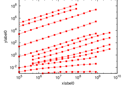
For the coupled symplectic maps (model A) numerical computations [33, 34], performed in a range , indicated a weak diffusion at , the authors fitted the data with a stretched exponential dependence. Here we extend these calculations and show the results in Fig. 12. One can see a strong decrease of the diffusion constant with , which for small is close to a power-law dependence
| (13) |
A similar value of the exponent was obtained from the statistics of Poincaré recurrences in the range [42]. We note that for model C the above equation implies . The value of the exponent is close to the value given by Chirikov and Vecheslavov [10, 11]. However, they calculated the diffusion indirectly by expressing it via an effective width of a separatrix layer of a nonlinear resonance with the additional relation , which was verified with the direct computations of the Arnold diffusion in systems with a few degrees of freedom. In fact, the value of is determined in [10, 11] via the computation of the period of oscillations around a separatrix layer of a nonlinear resonance that is related to the computation of LE. Due to this indirect method, Chirikov and Vecheslavov were able to obtain the variation of the Arnold diffusion constant by 50 orders of magnitude! On a scale of first 30 orders of magnitude the decay of the diffusion constant is well described by the power law with (see Fig. 1 in [11]). The main message of these amazing calculations is a non-exponential decay of , and hence of the chaos measure , with the decrease of nonlinearity parameter . This result is in a drastic difference from the asymptotic Nekhoroshev-like estimates based on the KAM theory [6, 7] which give exponential decrease of and as . Of course, there is no formal contradiction since the results for fast Arnold diffusion [11] are always obtained at small but finite values. However, an algebraic decrease with indicates on an existence of weak chaos component with relatively large measure. The heuristic arguments for this phenomenon were presented in [11]. According to the results of [11] one has for model A:
| (14) |
for . Here, is a dimensionless measure of the chaotic separatrix layer of the resonance between two nearby oscillators. For the range the decay of is compatible with the power law but this range of variation is not very large. The global dependence is fitted by the dependence of Eq. (5.8) in [11] which however has no complete theoretical explanation.
The reason why one can hardly compute the diffusion coefficient at smaller is clear from the inspection of the dependence of the variance on time in Fig. 12. For small one observes a normal diffusion only when the variance exceeds , below this value the diffusion looks like anomalous one with the variance proportional to a power of time. This means that a “random walk” inside the periodicity cell is highly correlated, while only cell-to-cell walk demonstrates a normal diffusion. For small the mean first passage time to the next cell becomes extremely large – nearly for , while for this mean passage time is of order or larger than the total integration time and only the anomalous diffusion is observed.

The obtained properties of diffusion should be contrasted to the properties of LEs, as both quantities give some characteristic times of the system. We have demonstrated that these times become extremely different for small non-integrabilities, as the Lyapunov exponent decreases rather weakly with while the diffusion constant drops much more rapidly. We interpret this as indication that chaos is mainly “local”, not leading to large deviations of variables. This picture corresponds well to the discussed above effective resonances as the origin of chaos: in the triple resonance described above in Section 4, the sum of all momenta is a conserved quantity, so that the chaotic dynamics like in Fig. 11 does not lead to a large deviation of momenta involved in the resonance. Indeed, there is strong chaotic dynamics inside the triplet resonance, but the sum of three resonant actions is a constant in the resonance approximation that would give a zero diffusion coefficient . However, the resonant approximation is not exact and it is destroyed by nonresonant terms and higher order perturbations that leads to a finite value of the diffusion . A mixture of strong chaos, which is however bounded due to an additional integral of motion, and a slow but unbounded diffusion produced by weak chaos makes the numerical computation of the diffusion rate a rather difficult task. In fact, usual very powerful methods discussed in [43], which allowed to compute as small diffusion rate as , are not working in such a situation and only computations at very long times allow to determine directly the value of .
The physical origins of the power law decay of the diffusion rate with (13) are still to be understood. The theoretical heuristic arguments presented in [11] assume that in the regime of weak chaos a trajectory follows mainly those chaotic resonant layers which have locally most large size. An optimization over various resonances leads to a certain power low decay for and which gives and respectively (we remind that for the Chirikov standard map [2, 11]). This theoretical value of the exponent is in a satisfactory agreement with the numerical value found at not very small values. However, at very small values of such arguments should be modified to fit an unknown dependence of resonance amplitudes in high orders of perturbation theory [11]. According to the heuristic arguments [11] the main contribution to diffusion is given by the resonances with an effective resonance harmonic numbers with a dimensionless measure of chaos inside one given resonance separatrix layer . We may argue that the number of such layers grows with at least as so that the total measure of weak chaos can be estimated as . This dependence is in a satisfactory agreement with the data of Fig. 8 (see the dashed curve there) and the empirical exponent value in (6). Thus we can say that our data for the measure of weak chaos are in a satisfactory agreement with the numerical results [11].
On the other hand, the origin of such a weak chaos component is still to be clarified. Indeed, the studies and arguments presented in [11] did not take into account the strong chaos based on triplet resonances which exists at arbitrary small . This strong chaos component emerges as the result of triple primary resonances but it is clear that a similar mechanism can work for higher order resonances which may be at the origin of the weak chaos component. On the other hand, the triple-like resonances of higher order in should lead to appearance of a certain number of trajectories with the LEs with that is, however, is not visible in the distribution of LEs in Figs. 6,7,8. It is however, possible that other tiny chaotic layers hide such contributions. Further studies are required to clarify these points especially in the regime with large . An indication on the complex internal structure of weak chaos provides Fig. 9 above, which demonstrates how a trajectory visits regions with different LEs along a very long evolution.
6 Spreading of chaos
Above we discussed the local properties of chaos computing the Lyapunov exponents and the diffusion rate in the regime when all nonlinear oscillators are populated in the initial state. Another type of question appears for the model C2 (3) when only one of few nearby oscillators are initially excited with the total energy and while all other oscillators have zero energy. Since the total energy is conserved we face the question on a possibility of energy spreading over the whole lattice of size . This is related to the question of ergodicity of large finite lattices at small energies. In the case when both nonlinear terms in the Hamiltonian (the local potential and the coupling) have the same power (e.g. the coupling has power instead of , such a model can be called model C44) then it is known that a thermalization takes place at arbitrary small total energy according to the arguments given in [40]. Of course, the time for such global ergodicity grows as a power of system size . For models with a nonlinear destruction of the Anderson localization, we have the terms with powers for local potential and for coupling in (3), which we call model C24. In this case it is found that a slow subdiffusive spreading over the lattice takes place up to very long times (see details in recent papers [18, 19, 20, 24, 25, 26, 27, 29, 40]). The model C2 corresponds to a new situation for energy spreading when the unperturbed integrable Hamiltonian is nonlinear and the coupling between nonlinear modes has higher nonlinearity. In contrast to the FPU problem, here the coupling between modes is local and the randomness in local nonlinear frequencies excludes any proximity to a full hidden integrability.


Let us assume that in model C2 with the above local initial conditions the energy spreads over the whole lattice of oscillators with an approximate energy equipartition over sites. After a rescaling of variables of this final state to a new time we come to the model C2 with and a homogeneous initial condition, discussed in the previous sections. In general, the probability of strong chaos in such a case scales as so that we expect local strong chaos to occur almost surely in a sufficiently long lattice. The same it true for the probability of weak chaos even if in this case the sum value of the exponents in is close to zero. Although the probability to observe chaos is high, it is important to note that this chaos is mainly local: some modes are chaotic, e.g. triplets discussed above, but other modes generally oscillate nearly quasiperiodically. Indeed, in a system with many degrees of freedom some modes can be chaotic while others can be close to integrable ones, without any contribution to the maximal LE. Thus, it is not obvious if the local strong chaos can allow spreading from initial local state over the whole lattice.
Let us present here simple estimates on the possible rate of such a spreading using results for the diffusion in the weak chaos component. We assume that a chaotic spreading populates the number of modes at time . Using rescaling given above we can argue that the new mode will be populated due to the weak chaos diffusion after a time scale . This gives us an effective local diffusion rate in with leading to the subdiffusive growth of the second moment :
| (15) |
For we obtain . However, our results for spreading, shown in Fig. 13, give approximately that corresponds to . We explain this difference in the following way. At the maximum time , reached in our numerical simulations, the energy spreads over a number of modes so that we have an effective which is only at the beginning of the decay with the exponent shown in Fig. 12(right panel), if we assume a simple relation , which however still may have an additional numerical factor. It is interesting to note that the case with corresponds to independence of on after rescaling that is the case for nonlinear model C44 (with both potentials having power 4 in (3)) where the spreading goes indeed with the exponent as it is shown in [40].
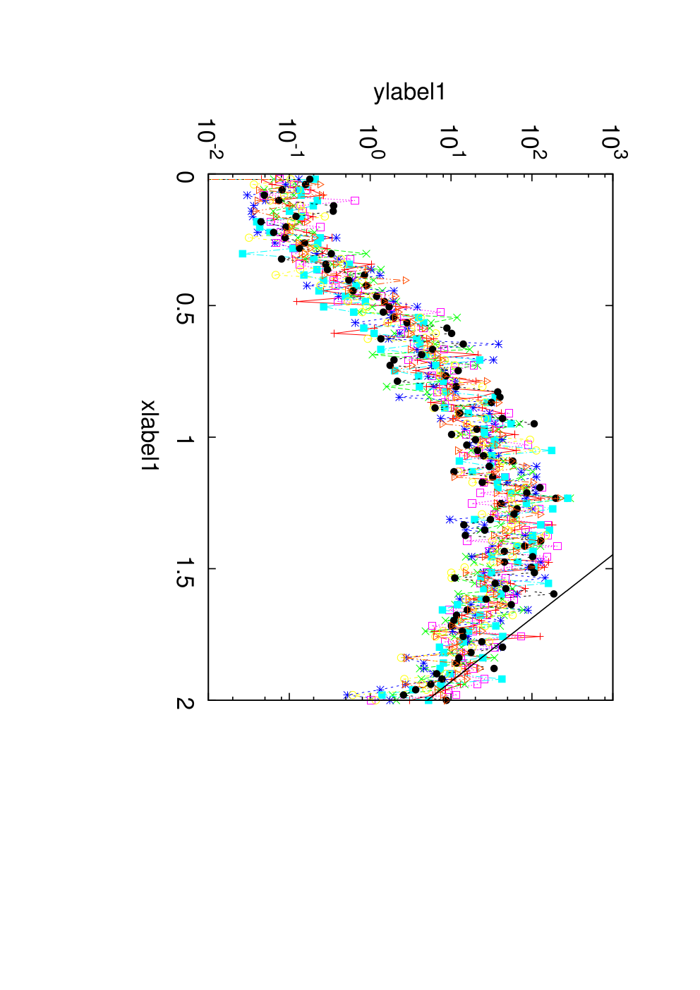
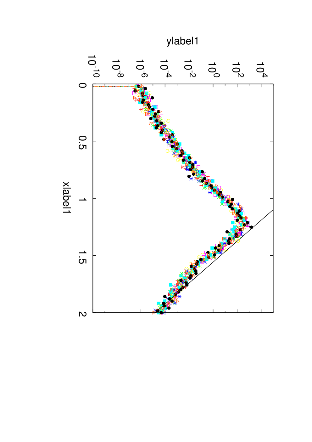
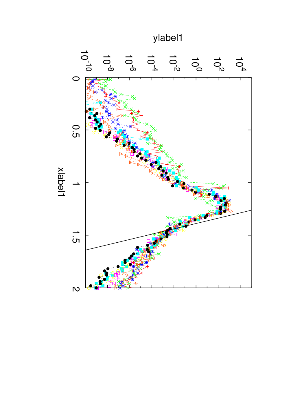
An indirect support to the view point according to which at we still did not reach the asymptotic spreading exponent is based on the numerical computation of the diffusion rate in an additional effective degree of freedom described by the equation , where are dynamical variables in model C1 (3). Solving these equations in parallel with the dynamical equations of motion for we determine the effective diffusion constant for each particle at . To suppress regular quasiperiodic oscillations we use the window averaging method described in [43] computing first the average over time interval and determining the diffusion for each via the relation . The computation is done for one trajectory with total time . The initial particle energies are chosen to be at . At we have the particle action and nonlinear frequency . The dependence of on frequency is shown in Fig. 14 for all values. In fact, gives us the spectral density of an effective noise produced by dynamical chaos. According to the results obtained for the modulational diffusion [43], the spectrum of is expected to have a plateau of width centered at the resonance , followed by an exponential drop . In the picture of triplet resonance we have . The data of Fig. 14 are in a satisfactory agreement with such a picture showing a decrease of the plateau size with the decrease of . The plateau is followed by an exponential drop. However, at the spectral width is still rather large being comparable with . At such spectral width even the oscillators that are not directly involved in the triplet resonance still will be affected by it. This is probably the reason why up to we have the spreading of chaos with the exponent corresponding to a usual diffusion in model C2. At the spectral width becomes notably smaller than unity but one needs to go to enormously large times to reach such effective values of during spreading of chaos. The value where there is a change in the dependence detected by Chirikov and Vecheslavov (see Fig. 1 in [11]) would require times at least as large as . Definitely such times remain out of reach of modern computations.
On the basis of presented results and discussions we can say that the spreading of chaos over the nonlinear oscillator lattice of model C2 (3) goes in a subdiffusive way (15) with the exponent up to times . In view of the result of Chirikov and Vecheslavov for the fast Arnold diffusion (13) [11] it is possible that the exponent will go down to at times . The properties of chaos spreading behind times remain absolutely unknown. During this anomalous slow growth of the wave packet size, the chaotic spreading follows the Arnold web of tiny chaotic layers propagating mainly along mostly thick ones. However, from time to time a trajectory can go inside thinner layers that leads to a strong drop of local diffusion and propagation rates, as well as a significant drop of LE (see, e.g., Fig. 9). It is quite possible that in this regime the energy distribution over the populated modes is still more or less homogeneous, as it is seen in Fig. 13, however, we expect this state to be not ergodic within these modes since chaos is presumably confined inside some “porous medium” of Arnold web with very complex structure and topology. In course of spreading, the energy per excited oscillator goes down to zero, so that such a process can be considered as an unusual non-ergodic cooling.
7 Slow diffusion in Hamiltonian systems as deterministic rheology
The spreading of chaos discussed above goes in a very slow way. In this section we explore a parallel with slow rheology processes characterized by small values of the Deborah number [44]
| (16) |
where is a time scale of local relaxation process and is a time of observation. The values of correspond to a liquid-like phase while appears for the solid phase. At our initial state with one or few excited oscillators we have the relaxation time to be comparable with the inverse LE , while the observation time of spreading is for our numerical simulations. Thus we have extremely small values of for our studies. The parallels with rheology processes, which are actively studied in soft matter and porous materials (see e.g [45, 46]), can be build on the basis of the following arguments: a)in rheology the flow processes are characterized by small values that is exactly the case for chaos spreading in model C2; b)often a spreading in a porous media is described by a nonlinear diffusion for a density [47]:
| (17) |
and it was shown recently that this equation gives a good phenomenological description of chaos spreading in nonlinear lattices; [26]; c)the Arnold web of chaotic resonance layers forms some kind of a porous media along which energy can spreads to larger and larger sizes. Recent experiments on gel formed by attractive colloidal hard spheres, suspended in an aqueous solvent, show that the spreading of gel is indeed well described by such type of a nonlinear diffusion equation (17) with a nonlinear flux term [48]. The theoretical models of rheology flow try to explain such a spreading by phenomenological statistical models with disorder and metastability (see e.g. [49, 50]). In contrast to such statistical models, our “rheology” of chaos spreading has purely dynamical and deterministic origin.
The value of given above should be considered as a global simplified estimate. It is also important to see how varies with time of spreading duration. For the model C2 we have and hence from (16) we find . Thus in this model at that argues in a favor of continuation of spreading at infinitely large times. The same criterion applied to the DANSE model, which describes the Anderson model with nonlinearity and was studied in [18], gives and thus still goes to zero in the limit of large times ( for DANSE). The above arguments show that for the nonlinearity studied in [26] we have and even for (see corresponding values of given in [26]). Indeed, the numerical results of [26] show an infinite spreading for such values of .
The above discussion shows that weakly nonintegrable many-body Hamiltonian systems give a new interesting example of rheology of chaotic dynamics. These systems are ruled by purely deterministic and rather simple Hamiltonian equations of motion. Exploring further statistical properties of such a deterministic rheology, generated by Hamiltonian many-body dynamics, is an important task for future studies.
8 Conclusion
In this paper we studied properties of non-integrable Hamiltonian lattices focusing on the regimes of very weak non-integrability. Our main results are scaling relations for the probability to observe strong chaos with the largest possible Lyapunov exponent. This probability is proportional to the product of the coupling parameter and the lattice length, while the Lyapunov exponent scales as a square root of the coupling constant. This behavior is explained by the observation that strong chaos is mainly due to resonances that appear when three neighboring sites occasionally have close frequencies. Because both the frequency mismatch and the characteristic time scale of the resonance are proportional to a square root of the perturbation parameter, the relations above directly follow from this scaling.
Furthermore, we confirm previous calculations showing that the diffusion time scale at weak non-integrability is much larger than the inverse Lyapunov exponent, and relate this to a weak diffusion inside the weak chaos component. The measure of this component decreases only algebraically with the strength of nonlinear coupling between nonlinear oscillators. The obtained results are in a good agreement with the fundamental finding of Chirikov and Vecheslavov [9, 10, 11] who first discovered this regime, with only algebraic decrease of the measure of chaos and diffusion rate at rather small perturbations, and named it the fast Arnold diffusion.
We also studied the spreading of chaos in such coupled nonlinear lattices showing that the spreading goes in an anomalous subdiffusive way. The link between the exponent of this spreading and the fast Arnold diffusion are also determined.
As already mentioned in the introduction, one has to distinguish weakly nonlinear and weakly non-integrable systems. There is, however, some analogy between the dynamics of weakly nonintegrable lattices studied in this paper and random lattices with weak nonlinearity [28, 30, 27, 18, 19]. We consider homogeneous lattices, where resonances appear randomly due to random choice of initial conditions. In random weakly nonlinear lattices resonances are determined by a lattice disorder. So in both cases one can expect that chaos is mainly sitting on resonances. For nonlinear homogeneous lattices, resonances can “move” as the energies on different lattice sites vary, while in weakly nonlinear disordered lattices the resonances are due to disorder and thus are “pinned”. The properties of chaos spreading in the latter case require separate investigations.
Acknowledgements.
We thank S. Fishman for useful discussions. A.P. thanks UPS, Toulouse for hospitality and support, DLS thanks Univ. of Potsdam for hospitality during visits in 2009, 2010. The work was supported by DFG via grant PI220/12. We thank ZEIK (Univ. Potsdam) and HLRS Stuttgart for providing the computer facilities.References
- (1) H. Poincaré, Acta Math. 13, 1 (1890)
- (2) B.V. Chirikov, Phys. Rep. 52, 265 (1979)
- (3) A.J. Lichtenberg, M.A. Lieberman, Regular and Chaotic Dynamics (Springer, New York, 1992)
- (4) V.I. Arnold, Dokl. Akad. Nauk SSSR 156, 9 (1964).
- (5) B.V. Chirikov, Research concerning the theory of non-linear resonance and stochasticity, Report 267, Inst. of Nuclear Phys., Novosibirsk (1969) [English CERN Trans. 71-40, Geneva (1971)].
- (6) N.N. Nekhoroshev, Usp. Mat. Nauk 32(6), 5 (1977).
- (7) P. Lochak, Uspekhy Mat. Nauk (Russian Math. Surv.) 47(6), 57 (1992).
- (8) V. Kaloshin and M. Levi, SIAM Review 50(4), 702 (2008).
- (9) B.V.Chirikov and V.V.Vecheslavov, KAM integrability, in Analysis, et cetera Eds. P.H.Rabinowitz and E.Zehnder, Research papers published in honor of Jurgen Moser’s 60th birthday, Academic Press, Inc., N.Y. p.219 (1990).
- (10) B.V.Chirikov and V.V.Vecheslavov, J. Stat. Phys. 71, 243 (1993).
- (11) B.V. Chirikov, V.V. Vecheslavov, Sov. Phys. JETP 85(3), 616 (1997) [Zh. Eksp. Teor. Fiz. 112, 1132 (1997)].
- (12) E. Fermi, J. Pasta, S. Ulam, and M. Tsingou, Los Alamos Report No. LA-1940, 1955 (unpublished); E. Fermi, Collected Papers, University of Chicago Press, Chicago, 1965, Vol. 2, p. 978.
- (13) A focus issue on “The “Fermi-Pasta-Ulam” problem – the first 50 years” (ed. by D. K. Campbell, P. Rosenau and G. Zaslavsky), CHAOS 15(1) (2005)
- (14) G. Gallavotti (ed.), The Fermi-Pasta-Ulam problem (Springer Lecture Notes in Physics vol. 728, 2008)
- (15) G. Benettin, R. Livi, A. Ponno, J. Stat. Phys. 135(5-6), 873 (2009)
- (16) D.L. Shepelyansky, Phys. Rev. Lett. 70, 1787 (1993).
- (17) M.I. Molina, Phys. Rev. B 58(19), 12547 (1998)
- (18) A.S. Pikovsky, D.L. Shepelyansky, Phys. Rev. Lett. 100(9), 094101 (2008)
- (19) I. Garcia-Mata, D.L. Shepelyansky, Eur. Phys. J. B 71(1), 121 (2009)
- (20) S. Flach, D.O. Krimer, C. Skokos, Phys. Rev. Lett. 102(2), 024101 (2009)
- (21) C. Skokos, D.O. Krimer, S. Komineas, S. Flach, Phys. Rev. E 79(5, Part 2), 056211 (2009)
- (22) M. Mulansky, K. Ahnert, A. Pikovsky, D.L. Shepelyansky, Phys. Rev. E 80, 056212 (2009)
- (23) Ch.Skokos, S. Flach, Phys. Rev. E 82(1), 016208 (2010)
- (24) S. Flach, Chem. Physics 375(2-3), 548 (2010)
- (25) T.V. Laptyeva, J.D. Bodyfelt, D.O. Krimer, Ch.Skokos, S. Flach, Europhys. Lett. 91(3), 30001 (2010)
- (26) M. Mulansky, A. Pikovsky, Europhys. Lett. 90, 10015 (2010)
- (27) M. Johansson, G. Kopidakis, S. Aubry, Europhys. Lett. 91(5), 50001 (2010)
- (28) D.M. Basko. Weak chaos in the disordered nonlinear Schroedinger chain: destruction of Anderson localization by Arnold diffusion. arXiv:1005.5033v1 [cond-mat.dis-nn] (2010)
- (29) D.O. Krimer, S. Flach, Phys. Rev. E 82(4, Part 2), 046221 (2010)
- (30) A. Pikovsky, S. Fishman. Phys. Rev. E 83, 025201 (2011).
- (31) W.-M. Wang and Z.Zhang, e-print arXiv:0805.3520 (2008).
- (32) J. Bourgain and W.-M. Wang, J. Eur. Math. Soc. 10, 1 (2008).
- (33) K. Kaneko, T. Konishi, Phys. Rev. A 40(10), 40 (1989)
- (34) T. Konishi, K. Kaneko, J. Phys. A 32, L715 (1990)
- (35) M. Falcioni, G. Paladin, A. Vulpiani, Europhys. Lett. 10(3), 201 (1989)
- (36) M. Falcioni, U. M. B. Marconi, A. Vulpiani, Phys. Rev. A 44, 2263 (1991)
- (37) A.J. Lichtenberg, A.M. Aswani, Phys. Rev. E 57(5), 5325 (1998)
- (38) E. Ott, Chaos in Dynamical Systems (Cambridge Univ. Press, Cambridge, 1992)
- (39) K. Ahnert and A. Pikovsky, Phys. Rev. E 79, 026209 (2009).
- (40) M. Mulansky, K. Ahnert, A. Pikovsky, Phys. Rev. E 83, 026205 (2011).
- (41) B.V. Chirikov, D.L. Shepelyansky, Sov. J.Nucl. Fiz. 36, 908 (1982)
- (42) D.L. Shepelyansky, Phys. Rev. E 82, 055202(R) (2010).
- (43) B.V. Chirikov, M.A. Lieberman, D.L. Shepelyansky, F. Vivaldi, Physica D 14, 289 (1985).
- (44) M. Reiner, “The Deborah number”, Phys. Today 17(1), 62 (1964).
- (45) A.Ya. Malkin, A.I. Isayev, Rheology: Concepts, Methods, & Applications ChemTech Publ., Toronto (2006).
- (46) M.A. Rao, Rheology of Fluid and Semisolid Foods: Principles and Applications, Springer, Berlin (2007).
- (47) G.I. Barenblatt, Scaling, Cambridge Univ. Press, Cambridge (2003).
- (48) G. Brambilla, S. Buzzaccaro, R. Piazza, L. Berthier, L. Cilelleti, “Highly nonlinear dynamics in a slowly sedimenting colloidal gel”, arXiv: 1102.5172 [cond-mat.soft] (2011) (to appear in Phys. Rev. Lett.)
- (49) P. Sollich, E. Lequeux, P. Hébraud, M.E. Cates, Phys. Rev. Lett. 78, 2020 (1997).
- (50) P. Sollich, Soft glassy rheology, in R. G. Weiss, P. Terech (Eds.), Molecular Gels: Materials with Self-Assembled Fibrillar Networks, p. 161, Springer, Berlin (2006).