HCOOCH3 as a probe of temperature and structure of Orion-KL Thanks: Based on observations carried out with the IRAM Plateau de Bure Interferometer. IRAM is supported by INSU/CNRS (France), MPG (Germany) and IGN (Spain).Thanks: A fits image of the HCOOCH3 integrated intensity map (Fig. 4) is only available in electronic form at the CDS via anonymous ftp to cdsarc.u-strasbg.fr (130.79.128.5) or via http://cdsweb.u-strasbg.fr/cgi-bin/qcat?J/A+A/ . All spectra can be obtained upon request to the authors.
Abstract
Context. The Orion Kleinmann-Low nebula (Orion-KL) is a complex region of star formation. Whereas its proximity allows studies on a scale of a few hundred AU, spectral confusion makes it difficult to identify molecules with low abundances.
Aims. We studied an important oxygenated molecule, HCOOCH3, to characterize the physical conditions, temperature and density of the different molecular source components. Methyl formate presents strong close rotational transitions covering a large range of energy and its emission in Orion-KL is not contaminated by the emission of N-bearing molecules. This study will help in the future 1) to constrain chemical models for the formation of methyl formate in gas phase or on grain mantles, 2) to search for more complex or prebiotic molecules.
Methods. To reduce the spectral confusion we used high resolution observations from the IRAM Plateau de Bure Interferometer in order to better isolate the molecular emission regions. We used twelve data sets with a spatial resolution down to 1.8 0.8. Continuum emission was subtracted by selecting apparently line free channels.
Results. We identify 28 methyl formate emission peaks throughout the 50 field of observations. The two strongest peaks, named MF1 and MF2, are in the Compact Ridge and in the South West of the Hot Core respectively. From a comparison with single dish observations, we estimate that we miss less than 15% of the flux and that spectral confusion is still prevailing as half of the expected transitions are blended over the region. Assuming that the transitions are thermalized, we derive the temperature at the five main emission peaks. At the MF1 position in the Compact Ridge we find a temperature of 80 K in a 1.8 0.8 beam size and 120 K on a larger scale (3.6 2.2), suggesting an external source of heating, whereas the temperature is about 130 K at the MF2 position on both scales. Transitions of methyl formate in its first torsionally excited state are detected as well and the good agreement of the positions on the rotational diagrams between the ground state and the vt=1 transitions suggests a similar temperature. The LSR velocity of the gas is between 7.5 and 8.0 km s-1 depending on the positions and column density peaks vary from 1.61016 to 1.61017 cm-2. A second velocity component is observed around 9-10 km s-1 in a North-South structure stretching from the Compact Ridge up to the BN object; ; this component is warmer at the MF1 peak. The two other C2H4O2 isomers are not detected and the derived upper limit for the column density is 31014 cm-2 for glycolaldehyde and 21015 cm-2 for acetic acid. From the 223 GHz continuum map, we identify several dust clumps with associated gas masses in the range 0.8 to 5.8 M☉. Assuming that the methyl formate is spatially distributed as the dust, we find relative abundances of methyl formate in the range 0.110-8 to 5.210-8. We suggest a relation between the methyl formate distribution and shocks as traced by 2.12 H2 emission.
Key Words.
Astrochemistry – ISM: molecules – Radio lines: ISM – ISM: individual objects: Orion-KL1 Introduction
The Orion Nebula is one of the most studied regions in the sky. It contains remarkable groups of bright, visible stars and, at the same time, it is an extremely rich region of star formation, up to very high masses. In addition, it is the closest high–mass star formation region to the Sun (Menten et al., 2007, 4147 pc,). It is thus the best source to investigate with very high spatial resolution the processes leading to star formation. However, Orion cannot be considered as the prototypical star-forming region in our Galaxy because it exhibits some unique characteristics which need to be understood before any generalization is made.
The Orion Kleinmann-Low nebula is an atypical region of the Orion Molecular Cloud 1 (OMC-1), which harbours one of the most luminous embedded IR sources of this region (Wynn-Williams et al., 1984, luminosity , ). Several molecular components (referred to as the Hot Core, Compact and Extended Ridges) and several IR sources or radio sources are associated with Orion-KL. The nature of the source(s) responsible for this IR emission is still poorly known and much debated. Many young stellar objects are still embedded in the dusty gas, including radio source I, a deeply embedded, high-mass young stellar object, which drives a bipolar outflow along a northeast-southwest axis (Beuther et al., 2005; Goddi et al., 2009; Plambeck et al., 2009) and presents a disk perpendicular to it (Matthews et al., 2010).
Another specificity of the Orion protocluster region is the presence of high speed shocks generated in the center of Orion-KL, reminiscent of an explosive event. From VLA velocity measurements, it was proposed that a very unique phenomenon had taken place some 500-1000 years ago: the close encounter, or collision, of two or more rather massives stars. The objects involved in such a dynamical interaction could have included the Becklin-Neugebauer object (BN) and sources I and n (Gómez et al., 2005; Rodríguez et al., 2005; Goddi et al., 2010). We might thus be observing a very recent and energetic event at the heart of the nebula, providing unique conditions for the study of a rich interstellar chemistry. With this scheme in mind, many molecules could have thus been released from the grain mantles because of dust heating or multiple shocks.
The search for complex or prebiotic molecules is difficult because of their relatively low abundance and line intensity. Especially in a very rich molecular source such as Orion-KL, high spectral confusion makes it difficult to detect the weakest lines. Among them, glycine (NH2CH2COOH, the simplest amino acid) has been searched for in the interstellar medium by many groups but has not been detected and only upper limits are given by the most sensitive studies (Combes et al., 1996; Guélin et al., 2008; Snyder et al., 2005, e.g.). On the other hand, observing abundant complex molecules is necessary to characterize the gas temperature and density of the various Orion-KL molecular source components. Observations of O- and N-bearing molecules show a clearly different spatial distribution. N-bearing molecules tend to peak to the north of the Hot Core while O-bearing molecules cover the Hot Core and the Compact Ridge (Guélin et al., 2008; Beuther et al., 2005; Friedel & Snyder, 2008).
Rotational temperature maps have been derived from interferometric observations of CH3OH (Beuther et al., 2005), NH3 (Wilson et al., 2000), both essentially focused on the Hot Core, and CH3CN (Wang et al., 2010); the intense lines of these abundant species require however to correct for opacity effects. Several single dish observations (Blake et al., 1987; Comito et al., 2005, e.g.) were also used to derive rotational temperatures towards the Hot Core and the Compact Ridge, which are supposed to be differentiated from their velocity structure. The spatial structure is lacking in these data, however.
In this paper we investigate the spatial structure and temperature distribution of Orion-KL from observations of the O-bearing methyl formate (HCOOCH3) molecule, which is relatively abundant in several interstellar hot cores and corinos, and especially abundant in Orion-KL (Blake et al., 1987; Kobayashi et al., 2007; Friedel & Snyder, 2008). In Sect. 2 we present our observations and the methyl formate frequency data base used in this work and we briefly describe the data reduction methodology. The results of our maps are presented in Sect. 3 together with details on the various molecular emission peaks identified in our maps. In Sect. 4, the temperature and molecular abundance across the entire V-shaped molecular structure linking IRc2 to BN are deduced from the rotational diagrams of the methyl formate molecule. In Sect. 5, upper limits on the abundance of methyl formate isomers are given. The dust and total mass and the mean gas density of the most prominent dust emission peaks are estimated from our continuum data in Section 6. The methyl formate fractional abundance is also estimated and briefly discussed in this same Section. We compare our results to previous studies in Section 7. In Sect. 8, the methyl formate distribution is discussed in the light of the complex structure of the Orion nebula. Conclusions are presented in the last Section.
2 Observations and methyl formate frequencies
2.1 Observations
We used twelve observational data sets obtained with the IRAM Plateau de Bure Interferometer (PdBI) towards the IRc2 region and its surroundings between 1996 and 2007. The bulk of the observations were obtained between 1999 and 2007. Table 1 lists the different parameters for each data set. The highest spatial resolution (1.79 0.79) was achieved in the period 2003 to 2007. Most observations used five antennas which were equiped with two SIS receivers operated simultaneously at 3mm and 1mm until 2006, then independently. 0420-014, 0458-020, 0528+134, 0605-085 and 0607-157 were used as phase and amplitude calibrators. The short–term atmospheric phase fluctuations were corrected at 1.3 mm on line. Tropospheric and radiometric phase corrections have been used since 1995 and October 2001, respectively, at the IRAM PdBI, based on the measured water line wings in the continuum emission observed with the 1.3 mm receiver and on the 22 GHz water line radiometers. The six units of the correlator allowed us to observe several data subsets with different bandwidths and spectral resolution which are also given in Table 1. For the highest spatial resolution the spectral resolution was around 0.84 km s-1 while some lower spatial resolution maps were obtained with 0.42 km s-1 spectral resolution. The uv coverage of these two data sets is shown in figure 1.
| Set 11 1 Sets 3 and 9 were centered on coordinates ( = 05h35m1420, = -05223600). Sets 1, 2, 4, 5, 6, 7, 8, 10, 11 and 12 were centered on coordinates ( = 05h35m1446, = -05223059). The observation velocity was 6 km s-1 for sets 1, 2, 6, 7, 8 and 8 km s-1 for the other sets. | Bandwidth | Date of | Confi- | HPBW | Spectral resolution | Flux conversion | Synthesized beam | Pixel size | ||
|---|---|---|---|---|---|---|---|---|---|---|
| (GHz) | observation22 2 Format: Month-Month/Year. | guration | () | (MHz) | ( km s-1) | (1 Jy beam-1) | ( ) | PA () | ( ) | |
| (1) | (2) | (3) | (4) | (5) | (6) | (7) | (8) | (9) | (10) | (11) |
| 1 | 80.502 - 80.574 | 10-11/1999 | CD | 60 | 0.625 | 2.33 | 4.6 K | 7.63 5.35 | 15 | 0.80 0.80 |
| 2 | 80.582 - 80.654 | 10-11/1999 | CD | 60 | 0.625 | 2.33 | 4.7 K | 7.62 5.23 | 16 | 0.96 0.96 |
| 3 | 101.178 - 101.717 | 33 3 Dates of observation: 12/2003, 01-12/2004, 03/2005, 01/2006. | BC | 50 | 0.625 | 1.85 | 15.8 K | 3.79 1.99 | 22 | 0.50 0.50 |
| 4 | 105.655 - 105.726 | 08-11/2005 | D | 48 | 0.3125 | 0.89 | 2.9 K | 7.13 5.36 | 9 | 1.40 1.40 |
| 5 | 105.785 - 105.856 | 08-11/2005 | D | 48 | 0.3125 | 0.89 | 2.9 K | 7.12 5.36 | 9 | 1.40 1.40 |
| 6 | 110.125 - 110.181 | 10/1996 | C | 46 | 0.15625 | 0.43 | 8.5 K | 5.85 2.02 | 8 | 0.54 0.54 |
| 7 | 203.331 - 203.403 | 10-11/1999 | CD | 25 | 0.625 | 0.92 | 7.0 K | 2.94 1.44 | 27 | 0.38 0.38 |
| 8 | 203.411 - 203.483 | 10-11/1999 | CD | 25 | 0.625 | 0.92 | 7.0 K | 2.94 1.44 | 27 | 0.32 0.32 |
| 9 | 223.402 - 223.941 | 44 4 Dates of observation: 12/2003, 01-12/2004, 03/2005, 01/2006, 11-12/2007. | BC | 23 | 0.625 | 0.84 | 17.3 K | 1.79 0.79 | 14 | 0.25 0.25 |
| 10 | 225.675 - 225.747 | 09-11/2005 | D | 22 | 0.3125 | 0.42 | 2.9 K | 3.63 2.26 | 12 | 0.70 0.70 |
| 11 | 225.805 - 225.942 | 09-11/2005 | D | 22 | 0.3125 | 0.42 | 2.9 K | 3.63 2.26 | 12 | 0.70 0.70 |
| 12 | 225.990 - 226.192 | 09-11/2005 | D | 22 | 0.3125 | 0.42 | 2.9 K | 3.63 2.25 | 12 | 0.70 0.70 |
2.2 Data reduction
We used the GILDAS package55 5 http://www.iram.fr/IRAMFR/GILDAS for data reduction. The continuum emission was subtracted in the data cubes by selecting line-free channels, discarding any contaminated (or doubtful) channels. Continuum emission in Orion-KL is essentially due to the thermal emission from the dust and to a weaker contribution from the free-free radiation of the gas. However, the contribution from the pseudo-continuum resulting from the superposition of many weak lines cannot be easily removed as it may depend on the spectral range analysed. The continuum emission is strong and spatially extended, varies with frequency, and reveals a clumpy structure at the highest spatial resolutions (see Fig.2 and Fig.16). As the center of the observations is not the same for all data sets, the continuum emission is better mapped toward the South at 223 GHz and toward the North at 225 GHz. Mapping the continuum emission is not obvious because of the high density of lines. It is difficult to isolate channels devoid of molecular lines. Nevertheless, we have been able to identify several channels (typically 4 to 22 by data sets) without line emission in our observations. All of these channels have been averaged and the average subtracted from each channel in the data cubes.
Finally, we have cleaned the data cubes, channel by channel, using the Clark method. Columns 9, 10 and 11 in Table 1 summarize the synthesized beam parameters for each dataset.


2.3 Interest of methyl formate observations
Methyl formate, one of three [C2H4O2] isomers, is relatively abundant towards Orion-KL, in view of its complexity. High angular resolution allows us 1) to isolate the different emission peaks of methyl formate and to investigate the gas structure, 2) and with large scale maps, to understand the overall Orion nebula structure (as discussed later in Section 8 of this work). High angular resolution also lowers the risk of spectral contamination by line-rich species such as C2H5CN, because the methyl formate distribution is different from that of N-bearing molecules (Blake et al., 1987; Kobayashi et al., 2007; Friedel & Snyder, 2008).
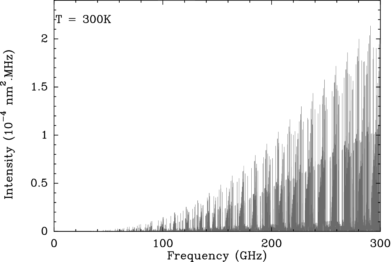
Methyl formate presents close rotational transitions (see Fig.3) with strong line strengths (S up to 50.2 D2 in our selection, see Tables 10 and 14). Several transitions covering an important range of energy can be observed at the same time. Comparison of these data obtained with identical spatial and spectral resolutions will allow an optimal estimate of the molecular gas physical conditions. The observed lines are all optically thin, which ease greatly their interpretation.
From a chemical point of view, formation of methyl formate on grain surfaces or in gas phase is still debated, as for many other complex species. The study of its spatial distribution, and its relative abundance with respect to other O-bearing molecules like methanol CH3OH, dimethyl ether CH3OCH3 and the two methyl formate isomers, glycolaldehyde CH2OHCHO and acetic acid CH3COOH, could help evaluate the different chemical models (Charnley & Rodgers, 2005; Bisschop et al., 2007; Garrod & Herbst, 2006; Garrod et al., 2008).
2.4 Methyl formate and isomers frequencies
Recently, Ilyushin et al. (2009) recalculated the rotational transitions of HCOOCH3 for the ground and first excited torsional states of this molecule. The JPL database66 6 http://spec.jpl.nasa.gov/home.html (Pickett, 1991; Pickett et al., 1998) is now updated (since April 2009) to include both the newly recalculated methyl formate frequencies and their own predictions (Drouin, B.J.). The methyl group, because of its three-fold internal rotation, leads to a series of thermally populated torsional levels which are split into two torsional substates with A and E symmetries. Previous data separated these two states while current data treat both substates simultaneously. In our study, we use the measured and predicted transitions coming from both Ilyushin’s table and the JPL database up to Eupper 650 K. Assuming HCOOCH3 lines are thermalized, we take into account transitions in their fundamental and first excited torsional states vt = 0 and vt = 1, respectively. Our observations confirm the detection of transitions of methyl formate in the first torsionally excited state (Kobayashi et al., 2007).
We also searched for the methyl formate isomers (see Sect. 5) and used Ilyushin et al. (2008) for the acetic acid and the CDMS database 77 7 http://www.astro.uni-koeln.de/cdms (Müller et al., 2001; Müller et al., 2005) for the glycolaldehyde transitions.
3 Mapping methyl formate emission (HCOOCH3) with the IRAM interferometer
The methyl formate molecule, HCOOCH3, allows us to trace the spatial distribution of one major oxygenated molecule in Orion-KL, especially in the direction of the Compact Ridge where high spatial resolution data are missing. We have adopted the Hot Core and Compact Ridge positions labelled in Beuther et al. (2005). Figure 4 shows our large scale, 1.79 0.79 beam size interferometric map of the HCOOCH3 line emission integrated over the line profile and on three different transitions: 114,8-103,7 A and E in vt =0 and 185,14-175,13 E in vt =1 (at 223465.340 MHz, 223500.463 MHz and 223534.727 MHz respectively) to improve the signal to noise ratio. It shows: (a) several main emission peaks labeled MF1 to MF28, and (b) an extended, V-shaped molecular emission linking the radio source I to the BN object.


3.1 Molecular emission peaks
We used the whole data set obtained with different frequencies and angular resolutions to model and investigate the properties of the methyl formate emission. The molecular emission peaks (MF1 to MF28) were determined from our highest angular resolution data (1.79 0.79) on the channel maps when they are present on at least three adjacent channels; they are listed in Table 2. The individual positions can vary by one pixel (0.25) depending on the HCOOCH3 transition. Two main molecular peaks, MF1 and MF2, are located toward the Compact Ridge and the Hot Core-SW respectively (Beuther et al., 2005; Friedel & Snyder, 2008, e.g references taken from). Emission peaks are present throughout the observed field and exhibit more or less extended structures. At some frequencies a molecular emission is also detected at the position of the millimeter source MM23 (Eisner et al., 2008).
| Position name | R.A (J2000) | Dec (J2000) |
|---|---|---|
| 05h35m | -0522 | |
| MF1 | 1409 | 367 |
| MF2 | 1444 | 344 |
| MF3 | 1431 | 372 |
| MF4 | 1415 | 293 |
| MF5 | 1412 | 277 |
| MF6 | 1450 | 326 |
| MF7 | 1405 | 423 |
| MF8 | 1420 | 461 |
| MF9 | 1411 | 433 |
| MF10 | 1468 | 289 |
| MF11 | 1445 | 306 |
| MF12 | 1418 | 346 |
| MF13 | 1409 | 325 |
| MF14 | 1416 | 370 |
| MF15 | 1372 | 140 |
| MF16 | 1373 | 191 |
| MF17 | 1444 | 240 |
| MF18 | 1346 | 308 |
| MF19 | 1366 | 315 |
| MF20 | 1346 | 366 |
| MF21 | 1364 | 393 |
| MF22 | 1361 | 413 |
| MF23 | 1501 | 348 |
| MF24 | 1468 | 367 |
| MF25 | 1520 | 387 |
| MF26 | 1438 | 494 |
| MF27 | 1392 | 503 |
| MF28 | 1400 | 353 |
The molecular emission peaks MF1, MF2, MF4-5 and MM23 are associated with the 4 main dust peaks identified at 223 GHz (see Fig. 16 in Sect. 6). However the continuum emission does not coincide exactly with the associated molecular line peak ( 0.1 to 1.2 and 0.03 to 1.8, except for MF2 where = 1.8 and = 2.9, for a beam size of 1.8 0.8). Since both continuum and line maps come from the same data sets the observed spatial separations cannot be ascribed to instrumental effects. de Vicente et al. (2002) report the same effect from their HC3N (10-9) lines observed in different vibrational levels. We conclude that even our best resolution is probably not sufficient to determine exactly the relative positions of molecular and dust emissions.
3.2 Velocity structure
Figure 5 presents the channel maps of the 223465.340 MHz line. Most of the peaks appear between 6 and 9 km s-1. However a linear structure is seen mainly toward the North at higher velocities (see discussion on MF1 and MF4 peaks in Sect. 3.5); it goes from MF5 to MF8 . There is no methyl formate emission at the Hot Core position at the usual 5 km s-1 velocity.
3.3 Critical density
We assumed that the HCOOCH3 transitions are thermalized at the five molecular emission peaks MF1 to MF5. From the H2 column densities measured at the continuum peaks associated to those positions (see Sect. 6 and Table 7) we find indeed n ncr 104-7 cm-3 for the detected lines at frequencies between 80 GHz and 226 GHz. To compute ncr, we have adopted the collision coefficients of H2O (Faure & Josselin, 2008) because of a similar dipole moment to HCOOCH3 ( = 1.8 D), and we have taken into account a multiplicative factor between 1 and 10 because HCOOCH3 is a larger molecule. Even if ncr would reach 107 cm-3 the critical density remains well below n (see Table 7).
3.4 Missing flux estimation
To estimate whether there is some flux missing in our data due to spatial filtering with the PdBI interferometer we have compared our PdBI spectra at 3 mm and 1 mm with IRAM 30-m telescope spectra. The PdBI spectra have been convolved with a Gaussian beam similar to the 30-m beam (25 at 3 mm and 11 at 1 mm). For all data sets the convolution was performed at the positions observed with the 30-m telescope. Error bars arising from the calibration and the pointing of the 30-m antenna fall within the typical range of 5 –10 .
In the Compact Ridge, comparison of our PdBI observations (which have a spatial resolution of 3.79 1.99 at the relevant frequencies) with the 30-m observations made at 101 GHz (Combes et al., 1996) indicates a ratio of missing flux of 3 and 15 measured from lines at 101370.505 MHz (133,11-132,12, E) and 101414.746 MHz (133,11-132,12, A) respectively. At 101477.421 MHz the 183,15-183,16E line is strongly blended with an intense H2CS transition (see Fig 6).
Concerning the Hot Core position, we also compared our PdBI observations (spatial resolution: 1.79 0.79) with the 30-m observations made at 223 GHz (J. Cernicharo, private communication). Chemically, this region exhibits an important molecular diversity implying a very high confusion level. All HCOOCH3 lines are blended either with another strong molecule or with a multitude of weaker lines, which makes it difficult to measure the exact missing flux. Using the 223500.463 MHz (114,8-103,7, A) line, we find that about 20 of the flux is missed. At 3 mm we estimate that we can miss between 4 and 15 of methyl formate emission flux ; this is determined from the lines at 101302.159 MHz (256,19-255,20, A) and 101370.505 MHz (133,11-132,12, E).

3.5 Observed parameters of the different HCOOCH3 peaks
Supposing that the gas rotational temperature does not exceed a few hundred Kelvin, we have searched for the 64 methyl formate transitions with Eupper 650 K. We have used the MAPPING GILDAS software to map and model the methyl formate source sizes, and the CLASS GILDAS software to determine the line parameters. The line frequencies, spectroscopic and observed parameters (v, v1/2, TB, W) at the MF1 to MF5 emission peaks are given in Tables 10 to 14. The observational results are briefly summarized below for the main molecular peaks shown in Figure 4.
MF1
is the main HCOOCH3 emission peak toward the Compact Ridge. It is present in all maps of detected HCOOCH3 transitions. The source sizes, estimated at half-peak flux density (see Table 10), increase with a lower spatial resolution from 3.0 2.0 at 223 GHz to 7.0 10.0 at 80 GHz. The line width clearly depends on the spatial and spectral resolutions. For instance, with the same beam ( 3 2) but using two different spectral resolutions, 1.85 km s-1 and 0.42 km s-1, we obtain v 3.6 km s-1 and 1.1 km s-1, respectively. Table 10 summarizes the line parameters for all detected, blended or not detected transitions in all data sets. We detected 20 lines, and observed 2 partially blended and 33 blended lines; 9 transitions were too faint to be detected. At both high spatial and spectral resolutions the 203 GHz, 223 GHz and 225 GHz methyl formate spectra display two components, one around 7.5 km s-1 and the other around 9 km s-1 (see fig. 7). The 2-velocity fit parameters are presented in Table 3. Both components have a narrow average line width of v1/2 1.7 km s-1. For the transitions observed with less resolution the second velocity component cannot be directly separated and the line widths are broader (v1/2 3.6 km s-1).


.
| Frequency | Transition | Eup | S2 | sigma | Component 1 | Component 2 | ||||||
|---|---|---|---|---|---|---|---|---|---|---|---|---|
| v1 | (v1/2)1 | TB1 | W1 | v2 | (v1/2)2 | TB2 | W2 | |||||
| (MHz) | (K) | (D2) | (K) | ( km s-1) | ( km s-1) | (K) | (K km s-1) | ( km s-1) | ( km s-1) | (K) | (K km s-1) | |
| 203435.554 | A | 155 | 5.3 | 0.09 | 7.6(0.9) | 1.6(0.9) | 6.40 | 10.6(1.6) | 9.3(0.9) | 2.2(0.9) | 0.88 | 2.1(1.6) |
| 203471.840 | E | 155 | 4.9 | 0.09 | 7.5(0.1) | 1.6(0.1) | 5.28 | 9.2(2.0) | 9.0(0.7) | 3.1(1.0) | 1.29 | 4.3(2.2) |
| 223465.340 | E | 50 | 2.1 | 0.17 | 7.6(0.1) | 2.0(0.2) | 10.74 | 22.5(1.9) | 9.5(0.2) | 1.5(0.3) | 3.17 | 5.0(1.7) |
| 223500.463 | A | 50 | 1.8 | 0.17 | 7.4(0.1) | 1.8(0.1) | 11.49 | 21.8(1.7) | 9.2(0.3) | 1.9(0.4) | 2.85 | 5.8(1.2) |
| 223534.727 | E, (vt=1) | 305 | 41.6 | 0.17 | 7.4(0.1) | 1.7(0.1) | 10.25 | 18.5(0.8) | 8.9(0.1) | 2.9(0.2) | 4.16 | 13.0(8.2) |
| 225855.505 | E | 36 | 3.1 | 0.10 | 7.6(0.1) | 1.2(0.1) | 6.84 | 9.1(0.1) | 9.2(0.1) | 1.1(0.1) | 2.56 | 2.9(0.1) |
| 225999.145 | E | 312 | 2.2 | 0.11 | 7.5(0.1) | 0.9(0.3) | 0.70 | 0.6(0.2) | 9.1(0.1) | 0.8(0.3) | 0.45 | 0.4(0.1) |
| Frequency | Transition | Eup | S2 | sigma | Component 1 | Component 2 | ||||||
|---|---|---|---|---|---|---|---|---|---|---|---|---|
| v1 | (v1/2)1 | TB1 | W1 | v2 | (v1/2)2 | TB2 | W2 | |||||
| (MHz) | (K) | (D2) | (K) | ( km s-1) | ( km s-1) | (K) | (K km s-1) | ( km s-1) | ( km s-1) | (K) | (K km s-1) | |
| 223465.340 | E | 50 | 2.1 | 0.17 | 8.0(0.1) | 1.9(0.3) | 3.83 | 7.7(2.5) | 10.2(0.8) | 3.7(1.0) | 1.66 | 6.6(2.7) |
| 223500.463 | A | 50 | 1.8 | 0.17 | 8.0(0.1) | 2.2(0.2) | 1.90 | 4.4(0.4) | 11.4(0.2) | 2.2(0.3) | 1.29 | 3.0(0.4) |
| 223534.727 | E, (vt=1) | 305 | 41.6 | 0.17 | 8.7(0.3) | 3.0(0.4) | 1.78 | 5.8(0.8) | 11.0(0.4) | 5.3(0.8) | 1.34 | 7.6(0.9) |
MF2
is the main HCOOCH3 emission peak toward the Hot Core region. This peak is present in all detected HCOOCH3 transitions. The source sizes, estimated at half-peak flux density (see Table 11 in Appendix A) increases with a lower spatial resolution from 2.5 1.2 at 223 GHz to 5.0 2.5 at 101 GHz88 8 Note that the lower spatial resolution of the detected lines at 80565.210 MHz and 105815.953 MHz does not allow us to identify individual sources. . This source appears to be more compact than MF1 in the Compact Ridge. Table 11 (in Appendix A) summarizes the line parameters for all detected, blended or not detected transitions in all data sets. We detected 14 lines and observed 3 partially blended and 40 blended lines; 7 transitions were too faint to be detected. The mean velocity is around 7.7 km s-1. As for clump MF1 the line widths depend on the spatial and spectral resolutions. With the highest spatial resolution (1.79 0.79) we find v1/2 2.4 km s-1 while for a resolution of 3.79 1.99, v1/2 4.1 km s-1; we did not take into account the partially blended line at 226061.796 GHz. The linewidths observed here are slightly broader than those of components 1 and 2 at the MF1 peak; as the lines are optically thin (see Sect. 4) this indicates a larger velocity spread in the source.
MF3
is a HCOOCH3 emission peak located in-between the two previous clumps. It often appears as an extension of the emission as most of our data do not allow us to isolate the emission peak. As for clumps MF1 and MF2, the linewidth is narrow; at 203 GHz and 223 GHz v1/2 1.7 km s-1. Table 12 (in Appendix A) summarizes the line parameters for all detected, blended or not detected transitions in all data sets. We detected 14 lines, and observed 3 partially blended and 26 blended lines; 21 transitions were too faint to be detected. The methyl formate velocity is around 7.7 km s-1.
MF4
is one of the main HCOOCH3 emission peaks lying at the North of the Compact Ridge. Table 13 (in Appendix A) summarizes the line parameters for all detected, blended or not detected transitions in all data sets. We detected 9 lines, and observed 4 partially blended and 28 blended lines; 23 transitions were too faint to be detected. As for clump MF1 the high spectral resolution line profiles show two components (see fig. 8). The 223 GHz methyl formate emission profiles are fitted with two components centered around 8.0 km s-1 and 11.4 km s-1 (Table 4). Both components have linewidths in the range (v1/2 1.9 - 3.7 km s-1).
MF5
lies near the emission peak MF4 and its size is similar to that of MF4. Two velocity components, visible with high spectral resolution only, are present in our data. However, we have not made any precise velocity identification of these components because they are more blended than those identified in the direction of MF4 and MF1. The unresolved emission is centered around 7.7 km s-1. We detected 9 methyl formate transitions and observed 3 partially blended and 28 blended lines. 24 other lines were too faint to be detected. All results from all data sets are summarized in Table 14 (in Appendix A).
3.6 Fraction of blended and detected lines
We have mentioned earlier that spectral confusion is a major problem toward Orion-KL. Confusion increases with frequency and it is more prevalent in our data at 223 GHz–225 GHz than at 101 GHz. Spectral confusion is present to some extent toward all the emission peaks identified in this work (MF1 to MF28).
We present here a rough estimate of the confusion level. From a visual inspection of our spectra, we believe that some line frequencies are contaminated by other lines, and noted a priori as blended, whereas at other line frequencies the spectrum appears free of contamination. To determine which lines are detectable in our data set we use the simple one-temperature model derived in Section 4 and compare the expected line intensity to the noise level. Of the detectable lines, a number, , are blended whereas others appear free of contamination.
For sources MF1, MF2 and MF3 all lines expected above 3 sigma and free of contamination are detected; this is a consistency check of the LTE model. To roughly quantify the effect of confusion in these sources we compute . We obtain the following results for temperatures derived from our rotational diagrams (see following Section):
- •
at the MF1 peak for T = 79 K,
- •
at the MF2 peak for T = 130 K,
- •
at the MF3 peak for T = 85 K
For sources MF4 and MF5, the presence of two velocity components makes the methyl formate lines broader and more difficult to detect. The number of detected lines is thus more imprecise, as for example some broad lines may be classified as blended instead of broadened by the dynamics. We get which is coherent with an increase of the confusion for broader lines. Some of the fainter lines expected to be detectable from the LTE model are not seen, especially in the data cubes around 225 GHz, which we attribute to an increased interferometric filtering of the quasi vertical MF4-MF5 structure in these cubes (compare the two uv coverages in Fig. 1).
The meaning of should not be overinterpreted because i) it depends on the LTE hypothesis, on the derived column density and temperature values and on the expected line profile; ii) it is not intrinsic to a molecule in a given source as it depends also on the frequency range and other observation parameters (noise level, spectral and spatial resolution, coverage). Note in addition that in the case of our dataset, the latter parameters vary from one datacube to another, so that is only an average value. It is however a first indication of the relative importance of the confusion problem - a similar indicator was given by Belloche et al. (2008) for their search and detection of amino acetonitrile in Sgr B2(N).
4 Temperatures and abundance of methyl formate towards the whole molecular V-shape
We assumed that all the lines are optically thin (calculated opacities are generally less than 0.05 and at most 0.1) and that the local thermodynamic equilibrium is reached for all positions (see Sect. 3.3), so that the kinetic temperature is equal to the excitation, rotational and vibrational temperatures. We estimated the rotational temperature and the column density of HCOOCH3 using the equation (Turner, 1991):
| (2) |
where,
Due to the CH3 group methyl formate is divided into two forms: A and E. Turner (1991) indicates that for A species: gi = 2 and gk = 1, and inversely for E species. We used gigk = 2 for all the transition lines.
We have made the rotational diagrams for two different spatial resolutions. One is based on the data with the highest spatial resolution (synthesized beam of 1.79 0.79 at 223 GHz ). The other one includes data at 101 GHz, 203 GHz and 225 GHz where the two first data sets are smoothed to the resolution of the third one (synthesized beam of 3.63 2.26) for the MF1 emission peak. The rotational temperatures and column density uncertainties, estimated by a least-square fit, are only based on the statistical weight of the detection measurements99 9 Error bars reflect only the uncertainties in the gaussian fit of the lines. Note that some points overlap because they correspond to lines with the same upper energy level Eup. (upper limits are not taken into account by the fit). The derived column densities are corrected for the beam filling factor.
Rotational diagram at the MF1 peak


We have made a rotational diagram for each velocity component. Figure 9 displays the diagrams obtained with the data at a 1.79 0.79 resolution (see set n∘9 in Table 1) and figure 10 the diagrams obtained with the data at a 3.63 2.26 resolution (see sets 7, 8, 10, 11 and 12 in Table 1). They show that the temperature of the 9.2 km s-1 component is higher (11250 K at high resolution and 16830 K at a lower resolution) than that of the 7.6 km s-1 component (792 K at high resolution and 11910 K at a lower resolution). We also note for both components that the temperatures are lower with the high spatial resolution, suggesting an external heating of the clump. The rotational diagram taking into account both components leads to an average rotational temperature of 100 K.
The derived column densities are given in Table 5. The column density derived with a high spatial resolution is larger than that derived with a lower spatial resolution.


Rotational diagram at the MF2 peak
Both rotational diagrams, for angular resolutions of 1.79 0.79 and 3.63 2.26 (see sets 9 and 3, 7, 8, 10, 11, 12 in Table 1, respectively), give comparable rotational temperatures, within the uncertainties. We obtain 1289 K and 14014 K, respectively (see Fig.11). The derived methyl formate column densities are given in Table 5.
Rotational diagram at the MF3 peak
The rotational temperature derived at a higher resolution is smaller (853 K) than that at a lower resolution (1033 K) (see Fig.12), suggesting external heating like for the MF1 peak. The derived methyl formate column densities are given in Table 5.
| Emission peaks | v1010 10 Towards MF1 and MF4 two different velocity components are identified but separate rotational diagrams could be made only for MF1 (see text) – for the other sources, velocity is a mean value of detected lines (see tables 11, 12 and 14 for details). | Trot1111 11 Error bars reflect only the uncertainties in the gaussian fit of the lines. | Nb | ||
|---|---|---|---|---|---|
| (km s-1) | (K) | (10cm-2) | |||
| (1.79 0.79) | (3.63 2.26) | (1.79 0.79) | (3.63 2.26) | ||
| MF1 | 7.6 | 792 | 11910 | 16.01.0 | 3.00.1 |
| MF1 | 9.2 | 11250 | 16830 | 6.82.1 | 1.60.1 |
| MF2 | 7.7 | 1289 | 14014 | 16.02.0 | 7.00.4 |
| MF3 | 7.7 | 853 | 1033 | 4.60.3 | 5.50.1 |
| MF4 | 8.2 | – | 1084 | – | 4.50.2 |
| MF5 | 7.8 | – | 1114 | – | 5.80.1 |
Rotational diagram at the MF4 peak
At 223 GHz, two velocity components are present as for the MF1 peak. Though two different upper energies are available, no rotational diagram at the resolution of 1.79 0.79 has been made because of the important error bars in the velocity decomposition. Fig.13 shows the rotational diagram at a 3.63 2.26 resolution. The derived gas temperature and column density are given in Table 5.
Rotational diagram at the MF5 peak
As for the MF4 peak and from the same above-mentioned argument no rotational diagram has been made at the resolution of 1.79 0.79.
Fig.14 shows the rotational diagram at a 3.63 2.26 resolution. The derived gas temperature and column density are given in Table 5. These values are close to those found at the nearby MF4 position.
The different temperatures obtained at different positions (MF1 to MF5) are most likely due to different physical conditions (see Sect. 8).

When we compare the methyl formate emission from different energy levels (see Fig.15), it is noticeable that for low upper state energies, the emission at the MF1 position is much stronger than at MF2. The emission at MF2 becomes stronger at higher energy levels.
5 Comparison with the other C2H4O2 isomers
Methyl formate (HCOOCH3), acetic acid (CH3COOH) and glycolaldehyde (CH2OHCHO) are three isomers among which acetic acid is the most stable. In a recent paper, Lattelais et al. (2009) have argued that the abundance ratio of isomers could be linked to their relative stability, except for some species as methyl formate. Indeed whereas methyl formate is known to be abundant in many molecular cores, glycolaldehyde has only been detected toward Sgr B2 (Hollis et al., 2000; Halfen et al., 2006, e.g.) and acetic acid is barely detected in hot cores (Shiao et al., 2010, e.g.).
We have searched for acetic acid and glycolaldehyde in our data sets (from upper energy levels of 18 K up to 452 K and of 25 K up to 646 K, respectively), using Ilyushin et al. (2008) for the acetic acid frequencies, but we detect neither of them. Assuming the rotational temperatures derived from our HCOOCH3 study, we have calculated upper limits for the column densities of these isomers at the MF1 and MF2 positions (Table 6). We find that the abundance of acetic acid is at least 50 times less than the methyl formate one and the abundance of glycolaldehyde at least 200-500 times less.
| Emission Peak | Temperature | Beam | N |
|---|---|---|---|
| (K) | ( ) | (cm-2) | |
| CH2OHCHO | |||
| MF1 | 78 | 1.79 0.79 | 2.41014 |
| MF1 | 120 | 3.79 1.99 | 2.81014 |
| MF2 | 128 | 1.79 0.79 | --1212 12 All the glycolaldehyde lines are blended, so that the upper limit is not significant. |
| MF2 | 140 | 3.79 1.99 | 3.51014 |
| CH3COOH | |||
| MF1 | 78 | 1.79 0.79 | 1.81015 |
| MF1 | 120 | 3.79 1.99 | 1.21015 |
| MF2 | 128 | 1.79 0.79 | 2.61015 |
| MF2 | 140 | 3.79 1.99 | 1.41015 |
6 Dust emission and characteristics of main clumps
Fig.2 shows that the continuum emission in the 101 to 225 GHz range is strong, extended and, from the highest frequency data, clumpy in places. In this Section we use the high spatial resolution and high signal-to-noise ratio achieved at 223 GHz (see Fig.16) to estimate, for the main clumps of dust emission, their masses, the mean projected column density and the H2 volume density. Combining our line results with our N estimates we further derive the relative abundance of the methyl formate molecule.
There are 4 main dust clumps in our 223 GHz map (Fig. 16): two, Cb and Ca, lie in the Compact Ridge and the Hot Core near the methyl formate peaks MF1 and MF2, respectively; Cc, in the north lies near MF4 and MF5; another clump, Cd, lies in the south near MM23. Each clump exhibits a complex spatial structure which is not fully revealed even with our 1.79 0.79 spatial resolution. In the Compact Ridge for instance, we have identified toward MF1 two clear continuum maxima (labelled Cb1 and Cb2 in Figure 16) which we consider, however, as one “single clump” (Cb). Ca, Cc and Cd are most probably not single entities as well, but we will consider them as roughly Gaussian clumps in our subsequent analysis. We first give below details on the equations used to derive the mean clump properties.
| Continuum | R.A (J2000) | Dec (J2000) | Adopted Td | sν1313 13 flux density per beam or brightness temperature. | N1414 14 estimated in a beam size of 1.79 0.79. | n1515 15 estimated in a beam size of 1.79 0.79 at a distance of 414 pc (Menten et al., 2007). | N/N1616 16 estimated at continuum and associated molecular peaks. The methyl formate column densities are derived from this work. | |
| Source | 05h35m | -0522 | (K) | (Jy beam-1) | (10cm-2) | (10cm-3) | (10-8) | |
| Ca | 1456 | 3150 | 200 | 0.49 | 5.4 | 7.3 | 0.6 | at continuum peak |
| 130 | 0.18 | 3.1 | 4.2 | 5.2 | at MF2 molecular peak | |||
| Cb | Cb1 1408 | 3673 | 80 | 0.18 | 5.0 | 6.8 | 3.1 | at continuum peak |
| Cb2 1401 | 3724 | |||||||
| 80 | 0.18 | 5.0 | 6.8 | 3.1 | at MF1 molecular peak | |||
| Cc | 1408 | 2750 | 110 | 0.12 | 2.4 | 3.3 | 0.3 | at continuum peak |
| 110 | 0.08 | 1.6 | 2.2 | 0.2 | at MF4 molecular peak | |||
| 110 | 0.08 | 1.6 | 2.2 | 0.5 | at MF5 molecular peak | |||
| Cd | 1403 | 4460 | 105 | 0.17 | 3.6 | 4.9 | 0.1 | at continuum peak |
| 105 | 0.17 | 3.6 | 4.9 | 0.1 | at MM23 molecular peak | |||

The flux density, Sν, from a dust cloud at frequency is given in the optically thin case by:
| (3) |
where is the dust opacity at frequency , Bν(T the Planck function, Td the dust temperature and the dust cloud solid angle. Estimating the dust column density and mass from the observables Sν and requires a dust opacity model and to know the variation of the extinction efficiency with frequency. This variation strongly depends on the wavelength range, the dust composition and its temperature. Mathis et al. (1977) suggested that the visible and UV interstellar extinction can be reproduced with a mixture of graphite and silicate grains and their model was extended to the infrared by Draine & Lee (1984). Draine & Lee (1984) showed that a mixture of silicate and graphite explains rather well the NIR and FIR observations and they showed that the FIR opacity varies as where is the wavelength. Of particular interest here is their estimate of the dust opacity at 125 m as a function of the visual absorption or the projected H gas density NH. They obtain NH(cm-2) which we extrapolate to the mm-wavelength regime, assuming that the extinction varies as ,
| (4) |
where we further assume the relation holds for molecular hydrogen with NH 2N. We are aware that the Draine & Lee (1984) data are rather typical of diffuse interstellar clouds and that dust coagulation as described by Ossenkopf & Henning (1994) for protostellar cores could be more appropriate. For an assumed central luminosity and outer envelope radius, the dust mass derived from a 1–D fit of the derived fluxes to the observed spectral energy distribution of the massive protostellar object W3IRS5 is 3 times lower with the Ossenkopf & Henning (1994) opacity profile than with the Draine & Lee (1984) profile (Luis Chavarria, private communication). However, the Ossenkopf & Henning (1994) opacities may be uncertain by a factor of at least 2 due to changes in the physical conditions and, given the additional dust to mass ratio uncertainty, derivation of the total gas mass in protostellar cores remains uncertain.
In this work we adopt a simple approach and combine equations 3 and 4 to derive in a straightforward manner the H2 projected density and hence the total mass. Using the observed peak flux density per synthesized beam, sν in Jy beam-1 (or source brightness temperature in K), and the Rayleigh-Jeans approximation, we derive, for the mean observing frequency of 223.65 GHz (1 Jy beam-1 = 17.3 K, for a HPBW of 1.79 0.79), the beam averaged projected density from
| (5) |
Assuming, for simplicity, that the dust clump is Gaussian with peak flux density sν and size determined from the 2-D Gaussian fits to the source half peak flux density, we derive the total gas mass in the entire Gaussian clump from the following equation (taking a mean molecular weight of 2.33 and adopting 414 pc as the Orion KL distance):
| (6) |
We use this equation to obtain the total gas mass present in our clumps (see Table 8).
All relevant gas clump parameters are gathered in Tables 7 and 8. They include the positions and names of the 4 main dust clumps as well as the adopted dust temperature (see details below), the peak flux in Jy beam-1, the projected and volumic densities and, see last 4 columns in Table 8, the clump sizes, total flux density and estimated total gas mass within the identified clumps. The methyl formate relative abundance at continuum and molecular peaks is also given in the last column of Table 7.
| Continuum | Nearby molecular | Adopted Td | Adopted clump surface1717 17 taken at half size | Mgas | Stotal |
|---|---|---|---|---|---|
| source | peak | (K) | ( ) | (M☉) | (Jy) |
| Ca | MF2 | 200 | 5.0 2.5 | 5.8 | 3.9 |
| Cb1818 18 Overall structure including Cb1 and Cb2. | MF1 | 80 | 4.0 2.5 | 4.3 | 1 |
| Cc | MF4, MF5 | 110 | 2.6 1.5 | 0.8 | 0.45 |
| Cd | MM23 | 105 | 3.0 1.5 | 1.4 | 0.8 |
The dust temperature is a crucial parameter in all of the above calculations. In order to estimate Td we assume that : (a) the gas-dust relaxation time is short (Draine, 2010; Tielens, 2005), and (b) the gas temperature is close to the rotational temperature Tr deduced from our methyl formate data. The gas-dust relaxation time is roughly given by 4 s / Tn(cm-3) which is 130 years for n cm-3 and TK around 100 K; therefore, dust thermalization should be well verified in Orion. Tr is rather well determined from our LTE multi-line analysis. Hence, it is reasonable to assume that both (a) and (b) are verified, thus Td Tr. Another complication arises because Td is not uniform throughout Orion as demonstrated by our continum maps, and our continuum and line peaks do not match exactly. The values of Td adopted here are given in Tables 7 and 8. They are taken from the rotational temperature obtained for the main gas peaks MF1, MF2, MF4, MF5 and MM23. There is also some uncertainty at the continuum peaks near both MF2 and MM23 because only 3 and 2 methyl formate lines were unanmbiguously detected in these directions (while many lines are present at the molecular peaks); in this case we used our best judgement to estimate Tr and thus Td.
The beam averaged projected density N lies in the range 2 to 5 1024 cm-2 corresponding to very large visual extinctions. The latter density is used to derive the volumic H2 density across the synthesized beam projected at the 414 pc distance of Orion-KL; it lies in the range 2 to 7 108 cm-3. Our derived densities are much higher than those found in the literature (Irvine et al., 1987; Persson et al., 2007; Mezger et al., 1990, e.g.). However, our spatial resolution is higher and the densities are similar if we take into account the beam dilution. Moreover, we find similar H2 density values when we use the continuum map of Beuther et al. (2004) and use their source and dust properties hypothesis.
Our individual clump masses vary from about 1 to 5 solar masses. We stress that these individual masses cannot be highly accurate because of various reasons. First, any Td uncertainty is directly translated into a mass uncertainty in our mass equations. Second, an uncertainty in the opacity wavelength dependence also results in a mass uncertainty; at 1.3 mm there is a 30% mass change when the extinction varies from a dependence to . Third, as explained earlier our clumps might not be Gaussian and our observed spatial structure might be even more clumpy than reported here. Another way to estimate our mass uncertainty is to derive the total gas mass for the entire clump from the equation, , where Sν is the flux density measured in Jy in our calibrated maps (see last column in Table 8). The derived masses differ from those obtained with equation 6 by about 9 to 30. Despite these uncertainties, we estimate that the total mass derived for all clumps identified here, about 12 solar masses, is meaningful. This mass reservoir could well be used in future star forming activity.
In the last column of Table 7 we also give the methyl formate relative abundance averaged over the synthesized beam in the direction of the 223 GHz dust emission peaks and of the molecular peaks. The relative abundances lie in the range 0.110-8 to 510-8 and show variations from one peak to another. Toward Cc and Cd, there are not enough detected molecular lines to estimate a precise methyl formate column density and we only give upper limits of the relative abundance. Toward Cb there is no difference in abundance between the molecular and continuum peaks, while there is a marked difference in the relative abundances measured toward the Hot Core (Ca) and the associated Hot Core-SW molecular peak (MF2). The largest methyl formate relative abundances are observed toward MF2 and MF1.
7 Comparison with previous studies
In this section we try to relate our results to some of the most comparable and recent other studies of Orion-KL. The large number of published works devoted to this region prevents us from being exhaustive. Therefore, we limit ourselves to the high (10) resolution studies of the continuum emission and methyl formate emission. There is a general agreement on space and velocity distribution and on column densities derived; however, our data show more details due to higher spatial and/or spectral resolution.
Methyl formate temperatures were often not derived by previous authors from their interferometric studies so we quote also for reference other temperature indicators at high resolution: dust color temperature, and methanol (CH3OH) and methyl cyanid (CH3CN) rotational temperatures. Methanol is interesting because this O-bearing species may be formed on grains (van der Tak et al., 2000, e.g.) like methyl formate, and, as stated previously it may also be a precursor of methyl formate. It may however suffer opacity problems, and its excitation is often more complex than LTE (Menten et al., 1988; Leurini et al., 2004, see e.g.). Methyl cyanide is a well-known probe of kinetic temperature (Boucher et al., 1980). But N-bearing species have a different distribution, so that temperatures derived from these molecules may thus differ from those derived from methyl formate.
Much work has been done on the other hand with single dish telescopes towards Orion-KL, and large surveys allow for the determination of a temperature of the region averaged over the beam, and sometimes for a decomposition into a few spectral features identified from their velocity profiles. We quote previous results on methyl formate and methanol avoiding, however, studies most affected by optical thickness effects. The HCOOCH3 temperatures we derive fall in the 60-220 K range found in these studies.
7.1 High resolution continuum maps
Our 1.3 mm continuum map differs from the Hot Core maps obtained with the SMA at 345 GHz and 690 GHz by Beuther et al. (2004) and Beuther et al. (2006) because we do not see any emission peak on source I and SMA1. We note that the Beuther et al. (2004) and Beuther et al. (2006) maps already show differences between each other. This could be due to the different spatial resolutions and/or to the different uv coverages used in these two works. Finally, we note that the SMA 870 m dust continuum maps of Tang et al. (2010) is much similar to our 223 GHz map obtained with a 1.79 0.79 resolution. Our map covers a more extended region of the southern Compact Ridge but all other clumps observed by us along the Ridge up to BN are also detected in the 0.8 0.7 SMA map. As also suggested by our 1.3 mm map, the 870 m dust emission map shows that there are at least two clumps in the Hot Core region. From their polarization study of the Hot Core and Compact Ridge Tang et al. (2010) suggest that the magnetic field is regulating star formation at large physical scales. Hence, all clumps identified here are probably intimately related with the Orion large scale magnetic field.
7.2 High resolution studies of methyl formate distribution and temperature
Our methyl formate emission peaks MF1, MF2 and MF4-5 1919 19 The MF5 emission peak corresponds to the IRc6 position in Friedel & Snyder (2008) and Beuther et al. (2005). are also present in the interferometric maps of Friedel & Snyder (2008) and Beuther et al. (2005) but the MF3 and MF4 peaks are less obvious in their data. Their maps, like ours, do not show any emission of this molecule towards the Hot Core around 5 km s-1.
The methyl formate observations of Friedel & Snyder (2008) made with the CARMA interferometer with a 2.5 0.85 beam size also reveal components at 7.6 km s-1 and 9.3 km s-1 towards the Compact Ridge region2020 20 Note that the Compact Ridge position defined in Friedel & Snyder (2008) is not the the same as that used in this study. Their IRc5 position is closer to our Compact Ridge position (1.5 away).. However the authors do not separate the two velocity components to derive the temperature and the column density. Their results agree with ours if we do not separate the two HCOOCH3 spectral components: Trot=101 K and N=1.51017 cm-2. Moreover methyl formate emission towards the Compact Ridge region has also been observed with BIMA by Liu et al. (2002) and Remijan et al. (2003). Their spatial and spectral resolutions do not allow them to see the two velocity components and they derive a temperature and a column density similar to those found by Friedel & Snyder (2008) and to ours when we combine the two components into one.
Hollis et al. (2003) also imaged methyl formate at high resolution (2.9 1.6) using the VLA at 45 GHz. The very low ( 6 K) energy of the upper state of the transition they observed shows that emission from the Compact Ridge is dominant, thus confirming the trend shown in our Fig.15. Despite their very good spatial resolution, their limited spectral resolution (1.36 km s-1 channel separation) allows them to detect only two broad peaks beside the Compact Ridge, corresponding to our MF2 and MF4-5 peaks. At the Compact Ridge peak (MF1), again summing up our two velocity components, our column density agrees with their value derived for a temperature of 100 K.
The interferometric map of methyl formate at 2 1.5 resolution integrated over velocities obtained with the Owens Valley interferometer by Blake et al. (1996) shows a reasonable global agreement with ours: Hot Core-SW and MF4-5 (IRc6) peaks are displaced from ours by 1, and their Compact Ridge peak lies 1.5 North of MF1; the emission around MF4-5 (IRc6) appears more intense and more extended, with peaks displaced by compared to ours.
7.3 Other temperature determinations
7.3.1 From dust infrared emission
Our temperature estimates lie in the range 80-170 K which is close to the range of (color) dust temperatures found by Wynn-Williams et al. (1984) from their 30 m and 20 m measurements, but they are lower than the temperatures they derive at shorter (and more optically thick) wavelengths. However, the temperature variations observed by Wynn-Williams et al. (1984) between the Hot Core, the Compact Ridge and IRc6 (MF4-5) are not ordered as in our study. This may be due to remaining opacity effects in the mid-infrared. In a more recent work Robberto et al. (2005) derived color temperatures in Orion-KL (excepting BN) of 125-140 K from 10 and 20 m observations, and higher values (200-230 K) from silicate features, using a simple “two-component” model for the IR emission.
7.3.2 From methanol and methyl cyanide high resolution studies
A comparison of our results with the temperatures derived from previous interferometric works on methanol (CH3OH) by Beuther et al. (2005) cannot be done toward the Compact Ridge and the Hot Core-SW because, unfortunately but not surprisingly, our two strongest methyl formate peaks correspond to areas where methanol is optically thick. It is only in the direction of MF4-MF5 (IRc6) that we observe some overlap with their temperature map: they find a somewhat higher temperature, around 180-240 K to be compared with our 110 K. Note that methanol emission is more extended than methyl formate and does not sample exactly the same gas, and methanol may be formed at least in part in the gas phase (Plambeck & Wright, 1988, e.g.); note also that a methanol maser has been identified by the latter authors at IRc6.
As N-bearing and O-bearing molecules clearly do not share the same spatial and velocity distribution (see e.g. their position velocity diagram showing the much broader velocity range of CH3CN emission), no simple comparison can be made of our work with the higher temperature values recently obtained by Wang et al. (2010) using CH3CN (190-620 K in the Hot Core and 170-280 K in the Compact Ridge).
Our temperatures and column densities derived from the analysis of the MF1 emission peak suggest an external heating towards the Compact Ridge. It is interesting to mention that recently Zapata et al. (2010) have also found some evidence for external heating towards the Hot Core. These two dense regions of the Orion-KL nebula seem to be associated with the dynamical event which occurred 500 years ago.
7.3.3 From single dish methyl formate and methanol studies
From a single dish measurement of the optically thin isotopologue 13CH3OH Blake et al. (1984) derived a rotational temperature of 120 K averaged over their 30 beam; this is close to the 140 K derived for CH3OH by Johansson et al. (1984) with a similar beam. Blake et al. (1987), also in a 30 beam, have attributed the methanol and methyl formate emissions to the Compact Ridge and derived rotational temperatures of 1463 K and 9010 K respectively, whereas a temperature of 16670 K was found in the Hot Core from their H2CO data. Within a 22-28 beam Menten et al. (1988) have derived from their CH3OH and 13CH3OH observations rotational temperatures of 109-147 K and 33 K respectively. Their CH3OH line profiles are interpreted as the superposition of a broad and a narrow component (the former marginally warmer by 10-20 K). This interpretation , aimed both at thermal emission and maser excitation, suggests that infrared radiation from the dust plays an important role in the excitation of methanol in addition to collisions. From a 325-360 GHz survey made with 20 resolution, Schilke et al. (1997) found rotational temperatures of 1883 K (methanol) and 983 K (methyl formate). More recently, at 350 m and with a 11 beam Comito et al. (2005) infer 220 K for the Hot Core, and 160 K for the Compact Ridge from CH3OH lines, and an almost identical value (220 K and 155 K) from H2CO. A somewhat lower temperature, 61 K, was found in a 40 beam for methyl formate by Ziurys & McGonagle (1993).
Very recently Herschel observations of 13CH3OH (and CH3OH) at 534 GHz and 1061 GHz made by Wang et al. (2011) determined Trot = 1052.6 K (resp. Trot = 1252.8 K) in the Compact Ridge; the Compact ridge was isolated from other spatial components in the 43 and 20 Herschel beams thanks to its velocity profile. A more elaborated transfer model developed for a spherical source with a temperature gradient provides a very good fit to the methanol population diagram of the Compact Ridge at both frequencies if it is externally heated. This conclusion well agrees with our findings.
8 Discussion on methyl formate distribution and Orion structure
The ÊOrion-KL region is located about 1 from the Trapezium OB stars at the heart of a large stellar cluster still in formation. Many remarkable objects Êhave been identified in this region (Irvine et al., 1987; Genzel & Stutzki, 1989; O’dell et al., 1993; O’dell, 2001; O’Dell & Henney, 2008; O’Dell et al., 2009, see e.g. reviews by). In this Section, we primarily try to correlate the HCOOCH3 distribution with several optical, NIR, MIR, X, radio continuum and radio line data, with the help of the ALADIN software2121 21 Centre de Données Astronomiques de Strasbourg, see:Ê http://aladin.u-strasbg.fr/aladin.gml andÊ http://simbad.u-strasbg.fr/simbad/. (Bonnarel et al., 2000) and the SIMBAD database8. We focus our discussion on the Compact Ridge and Hot Core regions as they contain the main methyl formate peaks in Orion-KL (MF1 and MF2, respectively).
8.1 Stars and YSOs
Orion-KL is a complex region, with a very high density of YSOs (Young Stellar Objects) and recently formed stars.
Putting together the remarkably detailed NIR pictures of Stolovy et al. (1998) and D. Rouan (private communication) together with the X picture (Getman et al., 2005; Grosso et al., 2005) and previous IR work (Greenhill et al., 2004; Hillenbrand & Carpenter, 2000; Lonsdale et al., 1982; Muench et al., 2002),Ê and including the IR polarization work of Simpson et al. (2006) we have been able to identify more than 34 probable stars or forming stars in the 0.5 region of methyl formate emission in Fig. 4. In this 0.058 pc wide field, this means a projected density of 156 objects arcmin-2 (1 object every 5) or objects pc-2. For comparison, Lada et al. (2004) determined stellar projected densities for deeply embedded sources reaching up to 3000 star pc-2 Êsouth of Orion-KL (this would mean 10 objects in the same 0.5 region of Fig. 4); for less embedded stars close to the Trapezium, the observed projected density is twice higher, up to 6000 star pc-2. With such a high density, one should Êalways keep in mind the possibility of chance projection effects Êin the following spatial comparisons.
Over small distance scales (a few or 1000-2000 AU), and with the exception of Parenago 1822/LBLS k at the center of the Compact Ridge (see discussion below), little correlation is seen between the methyl formate (MF) peaks and the stellar objects. Almost no association is obvious as well with the IRc sources, as seen on figure 17 which shows the position of the IRc sources from Shuping et al. (2004) with respect to the methyl formate emission. Over larger scales Ê(10 or 4500 AU) it seems, as discussed below, that the methyl formate distribution is closely linked to the presence of a few remarkable objects, in particular the “low-velocity” ÊSiO outflow whose origin is attributed to radiosource I by Goddi et al. (2009) and Plambeck et al. (2009), and linked to the matter (traced in CO and H2) ejected during the recent ( 500 yr) stellar collision or close interaction between the B-type star BN, and the I and n objects (at least) as proposed by e.g. Zapata et al. (2009). Long range effects due to heating, photodissociating photons or shocks are also possible from BN itself and source n. Note that our data do not allow us to separate the respective effects of source I from source SMA1 which has recently been identified by Beuther & Nissen (2008) as another candidate source for the high-velocity CO and H2 outflow.

8.2 HCOOCH3 and the "low-velocity" SiO outflow
As shown in Fig. 18 there is a striking complementarity of the 87 GHz SiO v=0 J=2-1 line map from Plambeck et al. (2009) with our methyl formate distribution. We consider that this fact is not fortuitous and points to some kind of direct connection between both species. The SiO traces the large “low-velocity” outflow originating from radio source I. As shown by various proper motion studies (Gómez et al., 2005; Rodríguez et al., 2005; Goddi et al., 2010) source I is moving towards the South-East (bottom left).
The HCOOCH3 distribution near MF2 (Hot Core-SW) may be due, to a large extent, to the recent sidewise “encounter” of this outflow with quiet dense gas resulting in shocks which in turn disrupt icy grain mantles and release new molecules.ÊThe Hot Core region would then be the prominent result of this sidewise encounter. With this picture in mind one expects a recent major increase in the release of molecules from grains in the Hot Core region and in the eastern side of the large scale V-shaped region mapped in MF in this work.
The Compact Ridge methyl formate distribution also matches the shape of the SiO outflow. In this area, the interaction is more frontal, the ouflowing matter coming more or less perpendicular to the border of the quiescent gas. The SiO outflow could be older than the stellar collision event. In that case the shock at the Compact Ridge would be older than the collision and be modified only by the recent motion of source I. Alternatively, the outflow could be linked to the stellar collision, or its trajectory might have encountered the Compact Ridge gas because of the recent proper motion of source I. In the first case, the release of molecules from grains would be older than 500 yr, in the latter case it would be more recent. Such a connection between the “low-velocity” outflow and the Compact Ridge has been proposed earlier (Irvine et al., 1987, see e.g.).
A shock from the I outflow can either release CH3OH rich ices, followed by gas phase chemistry leading to HCOOCH3 formation (Charnley & Rodgers, 2005), or directly release HCOOCH3 formed on the grain (Garrod & Herbst, 2006). The detailed chemical modelling is beyond the scope of the present study.
Ê

Ê
ÊÊÊÊÊÊÊÊÊÊÊÊÊÊ
8.3 HCOOCH3 and IR 11 map
In Fig. 19 we compare the methyl formate distribution with the 11 m map of Smith et al. (2005). There is a clear trend for Êthe MF emission peaks to lie outside the bright Ê11 m regions— it is especially true for the East branch of the V-shaped MF emission, which encompasses the Hot Core MF2 and goes from ÊMF7 to MF10. A notable apparent exception to this anticorrelation (but see below) is the main source MF1 located in the Compact Ridge.Ê
It has long been noted that there is a tendency for some molecular emission in Orion-KL, in particular NH3, Êto be anticorrelated with mid-IR emission (Genzel & Stutzki, 1989; Wynn-Williams et al., 1984, e.g.). Recently Shuping et al. (2004) reached a similar conclusion from their high resolution mid-IR map and the NH3 high resolution map of Wilson et al. (2000): they suggest that the NH3 emission comes from a foreground layer of interstellar matter, cold and dense enough to be seen in the mid-IR as an absorbing dark lane against a brighter background.
We propose that most of the methyl formate emission Êseen in places of low 11 m emission is also originating in this Êdark foreground material. In the case of MF1 in the Compact Ridge, there are indications that the methyl formate layer is also in the foreground material, but is thin enough to let the IR background radiation to be seen through it (see discussion on excited H2).
Ê
Ê Ê.
ÊÊÊÊÊÊÊÊÊÊÊÊÊÊ
Ê.
ÊÊÊÊÊÊÊÊÊÊÊÊÊÊ
8.4 HCOOCH3 and 2.12 H2 emission
MF1:
A most striking spatial correlation is observed between the methyl formate distribution at the MF1 peak and the 2.12 m H2 emission imaged by Lacombe et al. (2004) with adaptative optics (NACO) at the Very Large Telescope. This is shown in Fig. 20. Additional H2 pictures can be found in Stolovy et al. (1998) and Nissen et al. (2007).
We first note a global overlap of MF1 with a zone of excited H2 emission. Going into details, the MF1 methyl formate distribution departs from a simple elliptical shape, showing several extensions: 1) the MF1 peak corresponds to a local maximum of H2 emission, 2) there is a second peak at a North West position of the Compact Ridge (labeled NW in Fig. 20) in both tracers, 3) Two extensions of the MF map towards the South South East and West respectively of the Compact Ridge (labeled SSE and SSW in Fig. 20) correspond to two other peaks. These findings strongly support the association between MF and excited H2. At the North East of the Compact Ridge (position labeled NE in Fig. 20), MF overlaps the strong 2 m continuum emission which has been Êsubtracted and appears as a black zone in Fig. 20. This prevents a good comparison of the H2 emission in this area. However, inspection of the Subaru map (Fig. Ê21) confirms that there is also 2.12 m emission there.Ê
The North and South MF extensions have no counterpart at 2.12 m (only faint 2.12 m emission is present near N). They seem to be related to a different layer of emission, which appears as a North-South bar in the MF channel maps at velocities around or larger than 9 km s-1. Because such a structure does not show up in any optical or IR map, we consider it likely that the gas is on the far side of OMC-1, probably behind Êthe KL nebula itself.
Other peaks:
The methyl formate - excited H2 association observed in the MF1 area is also observed on a broader scale, especially, clockwise from the West, toward MF19, MF18-SW, MF21, MF27, MF8, MF23. However, some MF peaks have no excited H2 emission counterpart: for example, and most notably, there is no H2 emission at the MF2 (Hot Core-SW) peak; however excited H2 emission is present in its Southern part (Fig. Ê20 and 21). Conversely bright 2.12 m emission areas (e.g. East of the Hot Core, close to star LBLS t) do not exhibit MF emission.
To better understand the diversity of the observations the following explanations are worth considering:
- •
MF is seen associated with a 2.12 m emission if the shock related to the Orion-KL explosive event passes through interstellar material dense and cold enough so that grains have ice mantles. In that case the correlation observed toward MF1 is explained by the shock-induced release of methyl formate or its progenitor CH3OH from ice-coated grain mantles.
- •
The molecular production efficiency related to the shock may also be low in places, or cold grain mantles may be less abundant Ê(e.g. closer to the very luminous Trapezium OB stars located 1 SE of Orion-KL), so that the MF column density is undetectable.
- •
In some other places (e.g. around LBLS t) the 2.12 m emission geometry suggests that the emission is linked to the star and thus might be of a different nature.
- •
ÊMF may also peak in regions where it is released or produced by mechanisms (e.g. thermal heating) different from the shock generated by the explosive event.
- •
H2 emission may be hidden in some areas by a large column density of foreground dust.
The latter possibility is well illustrated by the comparison of the H2 2.12 m map of Lacombe et al. (2004) (Fig. Ê20) with the Subaru deep exposure (Shuping et al., 2004, Fig. Ê21, reproduced in extenso in). The larger extension of the H2 emission seen in the Subaru map indicates that a rather “ÊthinÊ” layer prevented some H2 peaks to be visible in the Lacombe et al. (2004) map. For a few H2 emission spots in this field Colgan et al. (2007) estimated indeed a foreground absorption corresponding to Av = 4-8. In the direction of the Compact Ridge, the NIR sources IRc4 and IRc5 are interpreted as reflection nebulae seen through holes of foreground matter (Shuping et al., 2004; Simpson et al., 2006); the larger size of these sources (hence of these holes) at 11 m compared to 2 m (continuum) is an additional indication of the relative thinness of the foreground matter.
On the contrary the MF2 peak would be a case where strong dust absorption hides all H2 2.12 m emission. Close to MF2, very large opacities are advocated to explain the non-detection of the bright source I (Greenhill et al., 2004, e.g.). Indeed from our continuum data (Sect. 6) we derive at both MF1 and MF2 peaks large N column densities (5 and 3.1 1024 cm-2 respectively); this corresponds to 1000, assuming standard dust opacities. Our interpretation of the contrasted situation at both peaks is that at the Compact Ridge (MF1), a shock hits the front side of a dense clump of matter, whereas at the Hot Core-SW (MF2), it hits the rear side (with respect to the observer). The presence close to MF2 of a H2O maser spot (Gaume et al., 1998, 053247.001-052427.81,), similar to other spots found in the Compact Ridge, strengthens the hypothesis that a shock is present there too.
The source of excitation of the H2 molecules is most likely linked to the global explosive event. Most of the H2 emission can be traced to a common center whose coordinates are given in Table 9 (e.g. Zapata et al. 2009 and refs. therein). Stolovy et al. (1998) analyse in detail two remarkable features which they call the “nested arcs” and the “bullets” (see their Fig. 4c),Ê and suggest that other H2 features in their map could be of similar nature but are less easily identified due to projection effects. If this is indeed the case, the comparison with these two features favourably seen in a more edge-on configuration sheds some light on the probable geometry of the shocked region at MF1, and how the shock might lead to the release of methyl formate from grain mantles; a detailed modelling at MF1 is however required.
Ê

Ê
ÊÊÊÊÊÊÊÊÊÊÊÊÊÊ
Ê

Ê
ÊÊÊÊÊÊÊÊÊÊÊÊÊÊ
Ê
| Object/place Ê | R.A. (J2000) | Dec. (J2000) | Precision Ê |
|---|---|---|---|
| 05h35m | -0522 | ÊÊ | |
| HCOOCH3 MF1 peak 2222 22 This study | ÊÊ05 35 14.09 | ÊÊ-05 22 36.7 | ÊÊ0.8 |
| P1822/LBLS k Ê2323 23 SIMBAD Ê | ÊÊ05 35 14.092 | ÊÊ-05 22 36.43 | ÊÊÊÊ |
| COUP 600 X source 2424 24 Grosso et al. (2005) | ÊÊ05 35 14.09 | ÊÊ-05 22 36.4 | ÊÊÊÊ |
| H2O supermaser Ê2525 25 Matveenko et al. (2000) after Greenhill et al. (2004) ÊÊ | ÊÊ05 Ê35 14.12 | ÊÊ-5 22 36.27 | ÊÊÊ |
| HC 438 2626 26 Eisner et al. (2008) Ê | ÊÊ05 35 14.09 | Ê-5 22 36.6 Ê | ÊÊÊÊ |
| CO Fingers Outflow Center 2727 27 Stolovy et al. (1998); Zapata et al. (2009) Ê | Ê05 35 14.37 | Ê-05 22 27.9 | 1.5 Ê |
| Proper motion center 2828 28 Gómez et al. (2005); Gómez et al. (2008); Rodríguez et al. (2005) | Ê05 35 14.35 | Ê-05 22 27.7 | Ê1 Ê |
8.5 Main Methyl Formate peak MF1 (Compact Ridge)
In addition to the correlation observed between the low-velocity outflow traced by SiO and the excited H2 emission at 2.12 m discussed above, some other remarkable objects are observed towards the main MF peak, MF1. The visible star Parenago 1822/LBLS k (Parenago, 1954; Parenago, 1997) is situated right in the middle of the MF1 methyl formate peak. ÊIt exhibits 1.3 mm continuum emission which is analyzed as disk emission by Eisner et al. (2008) under the name HC 438. Getman et al. (2005) derive an age of 22 000 yr and a small mass of 0.26 M☉. Another nearby remarkable object is the H2O “Supermaser” identified and studied by Matveenko et al. (2000), see also Demichev & Matveenko (2009) and Matveyenko et al. (2007). Table 9 gives the absolute position of this H2O source together with our methyl formate position and positions from other studies of nearby objects. Matveenko et al. (2000) estimate a very small mass of 0.007 M☉ for their H2O supermaser central source whose position is distinct from P1822/LBLS k. However, the proximity and youth of these two objects suggest that they might be a binary still in its forming phase.
P1822/LBLS k and associated supermaser could perhaps play a role in the observed distribution of methyl formate. Shocks are playing a central role in the Êvicinity of the H2O supermaser whose excitation and properties are best explained by molecular collisions in shocked dense gas clumps. These shocks may well have released the methyl formate or its precursor from grain mantles. However the methyl formate clumps cannot be always tightly associated with all the H2O maser spots because H2O maser emission traces only the hottest and densest pockets of gas.
We suggest that four phenomena, observed in an area as small as 5, may play a role in the release of the methyl formate molecule from ice grain mantles: i) bullets ejected 500 years ago (due to the BN-I-n encounter), ii) bipolar outflow from source I, iii) action from the star P1822/LBLS k, and iv) shocks linked to the excitation of the H2O supermaser. From a statistical point of view it seems unlikely that the above suggestions are unrelated. However, the relative importance of these four phenomena in the MF production, their relative timing and their causal relationship deserve further study.
9 Conclusions
We have studied the distribution of the complex O-bearing molecule Methyl Formate (MF) HCOOCH3 with medium to high angular resolution (7 to 2) using interferometric data from the IRAM Plateau de Bure Interferometer. Our main results and conclusions are the following:
- 1.
Our data sets include 21 well detected transitions of MF from Eup=25 K to Eup=618 K. A few more lines are present, still usable but partially blended with other lines. Only about 40 of the lines stronger than the weakest detected line appear free of blend. The line ares optically thin ( 0.1).
- 2.
We confirm the detection of vt=1 transitions. In this study, we used together vt=0 and vt=1 transitions to derive rotational temperatures.
- 3.
We identify at least 28 MF concentrations. The most intense emissions, MF1 and MF2, arise from the Compact Ridge and the Hot Core-SW respectively. The emission toward MF1 is much stronger than toward MF2 for low energy levels whereas the emission at MF2 becomes stronger at high energy levels.
- 4.
We have determined the MF temperature using rotational diagrams for the five main positions and deduced HCOOCH3 column densities assuming LTE. Temperatures cover the range 80 to 170 K, and column densities 1.61016 to 1.61017 cm-2.
- 5.
In the course of the MF data reduction, we had to produce and subtract maps of the continuum emission, using line free channels. We used these continuum maps to identify four major clumps Ca to Cd, for which we derived dust masses in the range 0.01 to 0.05 M☉ using a dust temperature equal to the MF rotational temperature. Assuming a gas-to-dust ratio of 100 the gas masses are in the range 1 to 5 M☉.
- 6.
MF gas velocities lie in the range 7-8 km s-1. At some places two different velocity components are clearly seen and the high velocity component (around 9-10 km s-1) has a linear North-South structure. We see no gas emission at the 5 km s-1 velocity usually reported for the Hot Core: the gas we observe there is slightly higher in velocity and probably of the same nature as the gas we observe for the Compact Ridge.
- 7.
We have searched for the two isomers of methyl formate but we did not detect them. We find an abundance ratio of less than 1/50 for acetic acid CH3COOH and less than 1/(200-500) for glycolaldehyde CH2OHCHO.
- 8.
We have correlated the MF1/Compact Ridge emission with other gas tracers and with various Orion objects. A very clear association is found with 2.12 m excited H2 maps. This tends to confirm a scenario of MF production involving the release of molecules from ice mantles, either MF itself or a precursor (CH3OH). Four possible origins have been identified for the excited H2 emission and the MF production: shock from the “low-velocity”outflow from source I, shock from a bullet ejected during the supposed collision-explosion event 500 yr ago (Zapata et al., 2009), action of the young forming star Parenago 1822/LBLS k , or from the nearby source (and possible companion of the star) responsible for the H2O supermaser (Matveenko et al., 2000).
We can not conclude yet which of these four likely processes dominates the MF production but all may have contributed.
To further analyze the Compact Ridge history more radio and IR high angular resolution images are needed. In the future, ALMA and adaptive optics on large ground based telescopes and space telescopes will provide the new data required to progress deeply in the understanding of the Orion-KL region.
The structure we find in Orion-KL might help to better understand the correlation previously found between cometary and interstellar ices (Bockelée-Morvan et al., 2000). In this correlation, sources of different nature a priori, "hot cores" on one side and a bipolar flow L1157 on the other side, both appeared as a good match of cometary ices. Shocks releasing molecules from icy grain mantles are in L1157 a major source of molecules in the gas phase . From the correlation we found between methyl formate and excited H2 emission, this might also be the case in Orion-KL as well as in other hot cores.
Acknowledgements.
We thank Laurent Margules and Brian Drouin for their spectroscopic knowledge and advices on HCOOCH3. We thank Thierry Jacq for his dataset at 80 GHz and 203 GHz, and Daniel Rouan and Nathan Smith for their H2 and 11 m maps. Valuable contributions from David Field are gratetfully acknowledged. We also thank Alexandre Faure for the discussion on lines in fundamental and excited torsional states. We thank the IRAM staff in Grenoble for their help to get and reduce the data. Finally we thank the anonymous referee for his helpful comments. This research has made use of the SIMBAD database and ALADIN software, operated at CDS, Strasbourg, France. This work was supported by CNRS national programs PCMI (Physics and Chemistry of the Interstellar Medium) and GDR Exobiology.References
- Belloche et al. (2008) Belloche, A., Menten, K. M., Comito, C., et al. 2008, A&A, 482, 179
- Beuther & Nissen (2008) Beuther, H. & Nissen, H. D. 2008, ApJ, 679, L121
- Beuther et al. (2004) Beuther, H., Zhang, Q., Greenhill, L. J., et al. 2004, ApJ, 616, L31
- Beuther et al. (2005) Beuther, H., Zhang, Q., Greenhill, L. J., et al. 2005, ApJ, 632, 355
- Beuther et al. (2006) Beuther, H., Zhang, Q., Reid, M. J., et al. 2006, ApJ, 636, 323
- Bisschop et al. (2007) Bisschop, S. E., Jørgensen, J. K., van Dishoeck, E. F., & de Wachter, E. B. M. 2007, A&A, 465, 913
- Blake et al. (1996) Blake, G. A., Mundy, L. G., Carlstrom, J. E., et al. 1996, ApJ, 472, L49+
- Blake et al. (1987) Blake, G. A., Sutton, E. C., Masson, C. R., & Phillips, T. G. 1987, ApJ, 315, 621
- Blake et al. (1984) Blake, G. A., Sutton, E. C., Masson, C. R., et al. 1984, ApJ, 286, 586
- Bockelée-Morvan et al. (2000) Bockelée-Morvan, D., Lis, D. C., Wink, J. E., et al. 2000, A&A, 353, 1101
- Bonnarel et al. (2000) Bonnarel, F., Fernique, P., Bienaymé, O., et al. 2000, A&AS, 143, 33
- Boucher et al. (1980) Boucher, D., Burie, J., Bauer, A., Dubrulle, A., & Demaison, J. 1980, Journal of Physical and Chemical Reference Data, 9, 659
- Charnley & Rodgers (2005) Charnley, S. B. & Rodgers, S. D. 2005, in IAU Symposium, Vol. 231, Astrochemistry: Recent Successes and Current Challenges, ed. D. C. Lis, G. A. Blake, & E. Herbst, 237–246
- Colgan et al. (2007) Colgan, S. W. J., Schultz, A. S. B., Kaufman, M. J., Erickson, E. F., & Hollenbach, D. J. 2007, ApJ, 671, 536
- Combes et al. (1996) Combes, F., Q-Rieu, N., & Wlodarczak, G. 1996, A&A, 308, 618
- Comito et al. (2005) Comito, C., Schilke, P., Phillips, T. G., et al. 2005, ApJS, 156, 127
- de Vicente et al. (2002) de Vicente, P., Martín-Pintado, J., Neri, R., & Rodríguez-Franco, A. 2002, ApJ, 574, L163
- Demichev & Matveenko (2009) Demichev, V. A. & Matveenko, L. I. 2009, Astronomy Reports, 53, 79
- Draine (2010) Draine, B. T. 2010, Physics of the Interstellar and Intergalactic Medium, ed. Draine, B. T.
- Draine & Lee (1984) Draine, B. T. & Lee, H. M. 1984, ApJ, 285, 89
- Eisner et al. (2008) Eisner, J. A., Plambeck, R. L., Carpenter, J. M., et al. 2008, ApJ, 683, 304
- Faure & Josselin (2008) Faure, A. & Josselin, E. 2008, A&A, 492, 257
- Friedel & Snyder (2008) Friedel, D. N. & Snyder, L. E. 2008, ApJ, 672, 962
- Garrod & Herbst (2006) Garrod, R. T. & Herbst, E. 2006, A&A, 457, 927
- Garrod et al. (2008) Garrod, R. T., Weaver, S. L. W., & Herbst, E. 2008, ApJ, 682, 283
- Gaume et al. (1998) Gaume, R. A., Wilson, T. L., Vrba, F. J., Johnston, K. J., & Schmid-Burgk, J. 1998, ApJ, 493, 940
- Genzel & Stutzki (1989) Genzel, R. & Stutzki, J. 1989, ARA&A, 27, 41
- Getman et al. (2005) Getman, K. V., Flaccomio, E., Broos, P. S., et al. 2005, ApJS, 160, 319
- Goddi et al. (2009) Goddi, C., Greenhill, L. J., Chandler, C. J., et al. 2009, ApJ, 698, 1165
- Goddi et al. (2010) Goddi, C., Humphreys, E. M. L., Greenhill, L. J., Chandler, C. J., & Matthews, L. D. 2010, ArXiv e-prints
- Gómez et al. (2008) Gómez, L., Rodríguez, L. F., Loinard, L., et al. 2008, ApJ, 685, 333
- Gómez et al. (2005) Gómez, L., Rodríguez, L. F., Loinard, L., et al. 2005, ApJ, 635, 1166
- Greenhill et al. (2004) Greenhill, L. J., Gezari, D. Y., Danchi, W. C., et al. 2004, ApJ, 605, L57
- Grosso et al. (2005) Grosso, N., Feigelson, E. D., Getman, K. V., et al. 2005, ApJS, 160, 530
- Guélin et al. (2008) Guélin, M., Brouillet, N., Cernicharo, J., Combes, F., & Wooten, A. 2008, Ap&SS, 313, 45
- Halfen et al. (2006) Halfen, D. T., Apponi, A. J., Woolf, N., Polt, R., & Ziurys, L. M. 2006, ApJ, 639, 237
- Hillenbrand & Carpenter (2000) Hillenbrand, L. A. & Carpenter, J. M. 2000, ApJ, 540, 236
- Hollis et al. (2000) Hollis, J. M., Lovas, F. J., & Jewell, P. R. 2000, ApJ, 540, L107
- Hollis et al. (2003) Hollis, J. M., Pedelty, J. A., Snyder, L. E., et al. 2003, ApJ, 588, 353
- Ilyushin et al. (2008) Ilyushin, V., Kleiner, I., & Lovas, F. J. 2008, Journal of Physical and Chemical Reference Data, 37, 97
- Ilyushin et al. (2009) Ilyushin, V., Kryvda, A., & Alekseev, E. 2009, Journal of Molecular Spectroscopy, 255, 32
- Irvine et al. (1987) Irvine, W. M., Goldsmith, P. F., & Hjalmarson, A. 1987, Astrophysics and Space Science Library, Vol. 134, Chemical abundances in molecular clouds, ed. D. J. Hollenbach & H. A. Thronson Jr., 561–609
- Johansson et al. (1984) Johansson, L. E. B., Andersson, C., Ellder, J., et al. 1984, A&A, 130, 227
- Kobayashi et al. (2007) Kobayashi, K., Ogata, K., Tsunekawa, S., & Takano, S. 2007, ApJ, 657, L17
- Lacombe et al. (2004) Lacombe, F., Gendron, E., Rouan, D., et al. 2004, A&A, 417, L5
- Lada et al. (2004) Lada, C. J., Muench, A. A., Lada, E. A., & Alves, J. F. 2004, AJ, 128, 1254
- Lattelais et al. (2009) Lattelais, M., Pauzat, F., Ellinger, Y., & Ceccarelli, C. 2009, ApJ, 696, L133
- Leurini et al. (2004) Leurini, S., Schilke, P., Menten, K. M., et al. 2004, A&A, 422, 573
- Liu et al. (2002) Liu, S., Girart, J. M., Remijan, A., & Snyder, L. E. 2002, ApJ, 576, 255
- Lonsdale et al. (1982) Lonsdale, C. J., Becklin, E. E., Lee, T. J., & Stewart, J. M. 1982, AJ, 87, 1819
- Mathis et al. (1977) Mathis, J. S., Rumpl, W., & Nordsieck, K. H. 1977, ApJ, 217, 425
- Matthews et al. (2010) Matthews, L. D., Greenhill, L. J., Goddi, C., et al. 2010, ApJ, 708, 80
- Matveenko et al. (2000) Matveenko, L. I., Diamond, P. J., & Graham, D. A. 2000, Astronomy Reports, 44, 592
- Matveyenko et al. (2007) Matveyenko, L. I., Graham, D. A., & Demichev, V. A. 2007, Memorie della Societa Astronomica Italiana, 78, 419
- Menten et al. (2007) Menten, K. M., Reid, M. J., Forbrich, J., & Brunthaler, A. 2007, A&A, 474, 515
- Menten et al. (1988) Menten, K. M., Walmsley, C. M., Henkel, C., & Wilson, T. L. 1988, A&A, 198, 253
- Mezger et al. (1990) Mezger, P. G., Wink, J. E., & Zylka, R. 1990, A&A, 228, 95
- Muench et al. (2002) Muench, A. A., Lada, E. A., Lada, C. J., & Alves, J. 2002, ApJ, 573, 366
- Müller et al. (2005) Müller, H. S. P., Schlöder, F., Stutzki, J., & Winnewisser, G. 2005, Journal of Molecular Structure, 742, 215
- Müller et al. (2001) Müller, H. S. P., Thorwirth, S., Roth, D. A., & Winnewisser, G. 2001, A&A, 370, L49
- Nissen et al. (2007) Nissen, H. D., Gustafsson, M., Lemaire, J. L., et al. 2007, A&A, 466, 949
- O’dell (2001) O’dell, C. R. 2001, in Revista Mexicana de Astronomia y Astrofisica, vol. 27, Vol. 10, Revista Mexicana de Astronomia y Astrofisica Conference Series, ed. J. Cantó & L. F. Rodríguez, 1–8
- O’Dell & Henney (2008) O’Dell, C. R. & Henney, W. J. 2008, AJ, 136, 1566
- O’Dell et al. (2009) O’Dell, C. R., Henney, W. J., Abel, N. P., Ferland, G. J., & Arthur, S. J. 2009, AJ, 137, 367
- O’dell et al. (1993) O’dell, C. R., Wen, Z., & Hu, X. 1993, ApJ, 410, 696
- Ossenkopf & Henning (1994) Ossenkopf, V. & Henning, T. 1994, A&A, 291, 943
- Parenago (1954) Parenago, P. P. 1954, Trudy Gosudarstvennogo Astronomicheskogo Instituta, 25, 3
- Parenago (1997) Parenago, P. P. 1997, VizieR Online Data Catalog, 2171, 0
- Persson et al. (2007) Persson, C. M., Olofsson, A. O. H., Koning, N., et al. 2007, A&A, 476, 807
- Pickett (1991) Pickett, H. M. 1991, Journal of Molecular Spectroscopy, 148, 371
- Pickett et al. (1998) Pickett, H. M., Poynter, I. R. L., Cohen, E. A., et al. 1998, Journal of Quantitative Spectroscopy and Radiative Transfer, 60, 883
- Plambeck & Wright (1988) Plambeck, R. L. & Wright, M. C. H. 1988, ApJ, 330, L61
- Plambeck et al. (2009) Plambeck, R. L., Wright, M. C. H., Friedel, D. N., et al. 2009, ApJ, 704, L25
- Remijan et al. (2003) Remijan, A., Snyder, L. E., Friedel, D. N., Liu, S., & Shah, R. Y. 2003, ApJ, 590, 314
- Robberto et al. (2005) Robberto, M., Beckwith, S. V. W., Panagia, N., et al. 2005, AJ, 129, 1534
- Rodríguez et al. (2005) Rodríguez, L. F., Poveda, A., Lizano, S., & Allen, C. 2005, ApJ, 627, L65
- Rohlfs & Wilson (2000) Rohlfs, K. & Wilson, T. L. 2000, Book Review: Tools of radio astronomy.- 3rd rev. ed. Springer, 2000, Vol. 120, 289
- Schilke et al. (1997) Schilke, P., Groesbeck, T. D., Blake, G. A., & Phillips, T. G. 1997, ApJS, 108, 301
- Shiao et al. (2010) Shiao, Y., Looney, L. W., Remijan, A. J., Snyder, L. E., & Friedel, D. N. 2010, ApJ, 716, 286
- Shuping et al. (2004) Shuping, R. Y., Morris, M., & Bally, J. 2004, AJ, 128, 363
- Simpson et al. (2006) Simpson, J. P., Colgan, S. W. J., Erickson, E. F., Burton, M. G., & Schultz, A. S. B. 2006, ApJ, 642, 339
- Smith et al. (2005) Smith, N., Bally, J., Shuping, R. Y., Morris, M., & Kassis, M. 2005, AJ, 130, 1763
- Snyder et al. (2005) Snyder, L. E., Lovas, F. J., Hollis, J. M., et al. 2005, ApJ, 619, 914
- Stolovy et al. (1998) Stolovy, S. R., Burton, M. G., Erickson, E. F., et al. 1998, ApJ, 492, L151+
- Tang et al. (2010) Tang, Y., Ho, P. T. P., Koch, P. M., & Rao, R. 2010, ApJ, 717, 1262
- Tielens (2005) Tielens, A. G. G. M. 2005, The Physics and Chemistry of the Interstellar Medium, ed. Tielens, A. G. G. M.
- Turner (1991) Turner, B. E. 1991, ApJS, 76, 617
- van der Tak et al. (2000) van der Tak, F. F. S., van Dishoeck, E. F., & Caselli, P. 2000, A&A, 361, 327
- Wang et al. (2010) Wang, K., Kuan, Y., Liu, S., & Charnley, S. B. 2010, ApJ, 713, 1192
- Wang et al. (2011) Wang, S., Bergin, E. A., Crockett, N. R., et al. 2011, ArXiv e-prints
- Wilson et al. (2000) Wilson, T. L., Gaume, R. A., Gensheimer, P., & Johnston, K. J. 2000, ApJ, 538, 665
- Wynn-Williams et al. (1984) Wynn-Williams, C. G., Genzel, R., Becklin, E. E., & Downes, D. 1984, ApJ, 281, 172
- Zapata et al. (2009) Zapata, L. A., Schmid-Burgk, J., Ho, P. T. P., Rodríguez, L. F., & Menten, K. M. 2009, ApJ, 704, L45
- Zapata et al. (2010) Zapata, L. A., Schmid-Burgk, J., & Menten, K. M. 2010, ArXiv e-prints
- Ziurys & McGonagle (1993) Ziurys, L. M. & McGonagle, D. 1993, ApJS, 89, 155
10
| N | Set | Frequency | Transition | Eup | S2 | sigma | v | v1/2 | TB | W | Nup/gup | Source size | Comments | |
|---|---|---|---|---|---|---|---|---|---|---|---|---|---|---|
| (MHz) | (K) | (D2) | (K) | ( km s-1) | ( km s-1) | (K) | (K km s-1) | (1012 cm-2) | ( x ) | PA() | ||||
| (1) | (2) | (3) | (4) | (5) | (6) | (7) | (8) | (9) | (10) | (11) | (12) | (13) | (14) | (15) |
| 1 | 1 | 80531.669(0.030) | E, (vt=1) | 216 | 0.6 | 0.05 | - | - | 0.15 | 0.6 | 1.04 | - | - | not detected |
| 2 | 1 | 80565.210(0.010) | E | 36 | 1.1 | 0.05 | 7.9(0.1) | 3.8(0.3) | 0.51 | 2.0(0.1) | 1.88 | 10.0x7.0 | 10 | detected |
| 3 | 1 | 80572.589(0.010) | A | 36 | 1.1 | 0.05 | 8.0(0.5) | 4.3(1.5) | 0.47 | 2.2(0.5) | 2.07 | 10.0x8.0 | 45 | detected |
| 4 | 2 | 80604.508(0.030) | E, (vt=1) | 288 | 0.2 | 0.09 | - | - | 0.31 | 1.3 | 6.73 | - | - | blend |
| 5 | 2 | 80652.521(0.010) | A | 83 | 1.0 | 0.09 | - | - | 0.74 | 3.0 | 3.10 | - | - | blend |
| 6 | 3 | 101202.806(0.010) | A, (vt=1) | 213 | 4.2 | 0.04 | 7.6(0.1) | 3.5(0.2) | 1.02 | 3.8(0.2) | 0.75 | - | - | partial blend |
| with U-line | ||||||||||||||
| 7 | 3 | 101210.208(0.004) | A | 187 | 0.04 | 0.04 | - | - | 0.12 | 0.4 | 8.68 | - | - | not detected |
| 8 | 3 | 101279.006(0.010) | E, (vt=1) | 212 | 4.0 | 0.04 | 7.8(0.1) | 3.4(0.1) | 1.18 | 4.3(0.1) | 0.89 | 5.5x3.5 | 84 | detected |
| 9 | 3 | 101289.471(0.010) | A, (vt=1) | 498 | 1.8 | 0.04 | - | - | 0.12 | 0.4 | 0.18 | - | - | not detected |
| 10 | 3 | 101302.159(0.010) | A | 219 | 11.1 | 0.04 | 7.6(0.1) | 3.9(0.4) | 3.11 | 12.8(1.0) | 0.95 | 5.0x3.5 | 26 | detected |
| 11 | 3 | 101305.506(0.010) | E | 219 | 11.1 | 0.04 | 7.8(0.2) | 3.7(0.4) | 2.65 | 10.4(1.0) | 0.77 | 5.5x3.5 | 20 | detected |
| 12 | 3 | 101318.966(0.010) | E, (vt=1) | 246 | 3.2 | 0.04 | 7.8(0.1) | 3.1(0.3) | 0.70 | 2.3(0.2) | 0.59 | 5.5x3.5 | 5 | detected |
| 13 | 3 | 101356.788(0.010) | A, (vt=1) | 263 | 3.5 | 0.04 | - | - | 0.59 | 2.1 | 0.49 | - | - | blend |
| 14 | 3 | 101370.505(0.010) | E | 60 | 3.2 | 0.04 | 7.9(0.1) | 3.7(0.1) | 3.78 | 14.7(0.1) | 3.78 | 5.0x3.5 | 5 | detected |
| 15 | 3 | 101414.746(0.010) | A | 60 | 3.2 | 0.04 | 7.8(0.1) | 3.6(0.1) | 3.73 | 14.3(0.1) | 3.68 | 5.0x3.5 | 5 | detected |
| 16 | 3 | 101418.330(0.001) | A, (vt=1) | 203 | 0.04 | 0.04 | - | - | 0.12 | 0.4 | 7.37 | - | - | not detected |
| 17 | 3 | 101477.421(0.010) | E | 111 | 1.8 | 0.04 | - | - | 9.31 | 33.2 | 15.17 | - | - | blend with H2CS |
| 18 | 3 | 101545.453(0.010) | A | 111 | 1.8 | 0.04 | 7.8(0.1) | 3.6(0.1) | 1.80 | 6.9(0.2) | 3.15 | 5.0x3.5 | 5 | detected |
| 19 | 3 | 101626.884(0.010) | E | 25 | 4.1 | 0.04 | - | - | 5.96 | 21.2 | 4.25 | - | - | blend with |
| HCOOCH3-A | ||||||||||||||
| 20 | 3 | 101628.149(0.010) | A | 25 | 4.1 | 0.04 | - | - | 5.47 | 19.5 | 3.91 | - | - | blend with |
| HCOOCH3-E | ||||||||||||||
| 21 | 4 | 105663.117(0.030) | E, (vt=1) | 412 | 0.4 | 0.02 | - | - | 0.06 | 0.1 | 0.20 | - | - | not detected |
| 22 | 4 | 105722.672(0.030) | E, (vt=1) | 230 | 0.5 | 0.02 | - | - | 0.11 | 0.2 | 0.32 | - | - | blend |
| 23 | 5 | 105810.803(0.030) | E | 142 | 0.2 | 0.03 | - | - | 0.11 | 0.2 | 0.79 | - | - | blend |
| 24 | 5 | 105815.953(0.030) | E | 10 | 0.2 | 0.03 | 7.6(0.1) | 2.2(0.2) | 0.39 | 0.9(0.1) | 3.55 | 10.5x7.5 | 6 | detected |
| 25 | 5 | 105832.067(0.030) | E | 142 | 0.2 | 0.03 | 7.9(0.1) | 1.6(0.2) | 0.20 | 0.4(0.1) | 1.58 | 10.5x7.5 | 6 | detected |
| 26 | 6 | 110153.652(0.010) | A, (vt=1) | 218 | 25.1 | 0.12 | - | - | 8.08 | 9.7 | 0.29 | - | - | blend with NH2D |
| 27 | 7 | 203349.158(0.006) | E | 416 | 0.2 | 0.09 | - | - | 1.73 | 2.8 | 5.77 | - | - | blend |
| 28 | 7 | 203378.812(0.007) | E | 416 | 0.2 | 0.09 | - | - | 5.64 | 9.2 | 18.94 | - | - | blend |
| 29 | 8 | 203427.575(0.100) | A, (vt=1) | 366 | 6.2 | 0.09 | 7.9(0.4) | 1.7(0.8) | 1.40 | 2.5(1.0) | 0.17 | 4.5x2.5 | 45 | detected |
| 30 | 8 | 203435.554(0.100) | A | 155 | 5.3 | 0.09 | 7.6(0.9) | 1.6(0.9) | 6.40 | 10.6(1.6) | 0.82 | 5.0x3.5 | 65 | detected |
| 31 | 8 | 203471.840(0.05) | E | 155 | 4.9 | 0.09 | 7.5(0.1) | 1.6(0.1) | 5.28 | 9.2(2.0) | 0.77 | 5.0x3.5 | 40 | detected |
| 32 | 9 | 223435.416(0.001) | A, (vt=1) | 237 | 1.8 | 0.17 | - | - | 3.66 | 6.7 | 1.38 | - | - | blend |
| 33 | 9 | 223465.340(0.050) | E | 50 | 2.1 | 0.17 | 7.6(0.1) | 2.0(0.2) | 10.74 | 22.5(1.9) | 4.00 | 3.0x2.0 | 0 | detected |
| 34 | 9 | 223500.463(0.001) | A | 50 | 1.8 | 0.17 | 7.4(0.1) | 1.8(0.1) | 11.49 | 21.8(1.7) | 4.61 | 3.0x1.5 | 0 | detected |
| 35 | 9 | 223534.727(0.100) | E, (vt=1) | 305 | 41.6 | 0.17 | 7.4(0.1) | 1.7(0.1) | 10.25 | 18.5(0.8) | 0.17 | 3.5x2.0 | 0 | detected |
| 36 | 9 | 223538.511(0.100) | E | 618 | 13.9 | 0.17 | - | - | 0.51 | 0.9 | 0.02 | - | - | not detected |
| 37 | 9 | 223592.231(0.100) | A | 618 | 13.9 | 0.17 | - | - | 0.91 | 1.7 | 0.05 | - | - | blend |
| 38 | 9 | 223618.470(0.007) | E, (vt=1) | 464 | 0.4 | 0.17 | - | - | 0.51 | 0.9 | 0.90 | - | - | not detected |
| 39 | 9 | 223624.496(0.100) | E | 463 | 11.7 | 0.17 | 7.7(0.3) | 1.8(0.6) | 0.68 | 1.3(0.4) | 0.04 | - | - | partial blend |
| 40 | 9 | 223634.916(0.100) | A | 463 | 11.7 | 0.17 | - | - | 2.06 | 3.8 | 0.12 | - | - | blend |
| 41 | 9 | 223642.180(0.001) | E | 63 | 0.1 | 0.17 | - | - | 4.08 | 7.4 | 32.97 | - | - | blend |
| 42 | 9 | 223645.342(0.001) | A | 63 | 0.1 | 0.17 | - | - | 1.66 | 3.0 | 11.23 | - | - | blend |
| 43 | 9 | 223651.592(0.007) | E, (vt=1) | 573 | 0.7 | 0.17 | - | - | 1.35 | 2.5 | 1.25 | - | - | blend |
| 44 | 9 | 223676.472(0.006) | A, (vt=1) | 593 | 3.0 | 0.17 | - | - | 2.09 | 3.8 | 0.47 | - | - | blend |
| 45 | 9 | 223782.081(0.007) | E, (vt=1) | 543 | 7.0 | 0.17 | - | - | 0.51 | 0.9 | 0.05 | - | - | not detected |
| 46 | 9 | 223821.523(0.002) | E | 409 | 8.2 | 0.17 | - | - | 2.31 | 4.2 | 0.19 | - | - | blend |
| 47 | 9 | 223854.201(0.100) | A | 409 | 10.1 | 0.17 | - | - | 4.63 | 8.4 | 0.31 | - | - | blend |
| 48 | 10 | 225689.371(0.008) | A, (vt=1) | 562 | 3.0 | 0.13 | - | - | 12.20 | 12.6 | 1.57 | - | - | blend |
| 49 | 10 | 225696.842(0.100) | E, (vt=1) | 307 | 50.2 | 0.13 | - | - | 16.8 | 17.4 | 0.13 | - | - | blend |
| 50 | 10 | 225702.857(0.100) | A, (vt=1) | 304 | 46.8 | 0.13 | - | - | 20.09 | 20.8 | 0.16 | - | - | blend |
| 51 | 10 | 225727.506(0.100) | A, (vt=1) | 224 | 3.1 | 0.13 | - | - | 4.04 | 4.2 | 0.50 | - | - | blend |
| 52 | 10 | 225727.506(0.100) | A, (vt=1) | 224 | 3.1 | 0.13 | - | - | 4.04 | 4.2 | 0.50 | - | - | blend |
| 53 | 11 | 225855.505(0.100) | E | 36 | 3.1 | 0.10 | 7.6(0.1) | 1.2(0.1) | 6.84 | 9.1(0.1) | 1.08 | 5.5x4.5 | 5 | detected |
| 54 | 11 | 225900.684(0.100) | E | 36 | 3.1 | 0.10 | - | - | 12.74 | 13.2 | 1.57 | - | - | blend with HDO |
| 55 | 11 | 225928.659(0.100) | A | 36 | 3.1 | 0.10 | - | - | 11.42 | 11.8 | 1.41 | - | - | blend |
| 56 | 11 | 225928.659(0.100) | A | 36 | 3.1 | 0.10 | - | - | 11.42 | 11.8 | 1.41 | - | - | blend |
| 57 | 12 | 225999.145(0.100) | E | 312 | 2.2 | 0.11 | 7.5(0.1) | 0.9(0.3) | 0.70 | 0.6(0.2) | 0.10 | 5.0x3.5 | 0 | detected |
| 58 | 12 | 226061.796(0.100) | E, (vt=1) | 321 | 4.0 | 0.11 | 7.6(0.2) | 1.0(0.5) | 0.72 | 0.8(0.3) | 0.07 | 5.5x3.5 | 25 | detected |
| 59 | 12 | 226077.920(0.001) | E | 39 | 0.3 | 0.11 | - | - | 2.62 | 2.7 | 3.53 | - | - | blend |
| 60 | 12 | 226081.175(0.002) | A | 312 | 1.8 | 0.11 | - | - | 0.71 | 0.7 | 0.14 | - | - | blend |
| 61 | 12 | 226087.718(0.007) | A, (vt=1) | 450 | 4.3 | 0.11 | - | - | 0.82 | 0.8 | 0.07 | - | - | blend |
| 62 | 12 | 226090.301(0.100) | E, (vt=1) | 303 | 47.0 | 0.11 | - | - | 9.62 | 9.6 | 0.08 | - | - | blend |
| 63 | 12 | 226112.470(0.007) | A, (vt=1) | 450 | 2.1 | 0.11 | - | - | 0.33 | 0.3 | 0.05 | - | - | not detected |
| 64 | 12 | 226125.600(0.001) | A | 39 | 0.3 | 0.11 | - | - | 4.04 | 4.2 | 5.49 | - | - | blend |
Notes: (1) Numbering of the observed transitions with Eupper 650 K. (2) Reference number of the corresponding data set (see Table 1). (3) Frequencies and uncertainties taken from Ilyushin et al. (2009) and from the JPL database (http://spec.jpl.nasa.gov/). (4) Transitions in ground state (vt=0). Transitions in torsional levels (vt=1) are specified. (5) Energy of the upper level. (6) Line strength calculated by Ilyushin et al. (2009). For the transitions coming from the JPL database, the line strength is calculated from the formulae of Pickett et al. (1998). (7) Noise estimated from spectrum (1). (8) Lines with number 30, 31, 33, 34, 35, 41, 53 and 57 are decomposed. Only the first component is given here, other components are given in Table 3, except for lines 29, 39 and 58 because of the blend with the second component. (8), (9), (10) and (11) Velocity, linewidth at half intensity, brightness temperature and integrated intensities. The uncertainties are estimated with the CLASS software. (12) Column densities of the upper state of the transition with respect to the rotational degeneracy (2Jup+1). (13) and (14) Source size estimated at half flux density from detected transitions with spatial resolution allowing to isolate the source. (15) Blended lines are specified.
Appendix A Transitions of methyl formate observed with the Plateau de Bure Interferometer towards positions MF2 to MF5 in Orion-KL.
The following tables summarize the line parameters for all detected, blended or not detected transitions of the methyl formate molecule (HCOOCH3) in all our PdBI data sets towards the emission peaks MF2 to MF5. \longtabL1
| N | Set | Frequency | Transition | Eup | S2 | sigma | v | v1/2 | TB | W | Nup/gup | Source size | Comments | |
|---|---|---|---|---|---|---|---|---|---|---|---|---|---|---|
| (MHz) | (K) | (D2) | (K) | ( km s-1) | ( km s-1) | (K) | (K km s-1) | (1012 cm-2) | ( x ) | PA() | ||||
| (1) | (2) | (3) | (4) | (5) | (6) | (7) | (8) | (9) | (10) | (11) | (12) | (13) | (14) | (15) |
| 1 | 1 | 80531.669(0.030) | E, (vt=1) | 216 | 0.6 | 0.03 | - | - | 0.09 | 0.4 | 0.69 | - | - | not detected |
| 2 | 1 | 80565.210(0.010) | E | 36 | 1.1 | 0.03 | 7.9(0.3) | 4.4(0.5) | 0.24 | 1.1(0.1) | 1.04 | - | - | detected |
| 3 | 1 | 80572.589(0.010) | A | 36 | 1.1 | 0.03 | - | - | 0.30 | 1.3 | 1.22 | - | - | blend |
| 4 | 2 | 80604.508(0.030) | E, (vt=1) | 288 | 0.2 | 0.10 | - | - | 8.03 | 35.3 | 182.73 | - | - | blend |
| 5 | 2 | 80652.521(0.010) | A | 83 | 1.0 | 0.10 | - | - | 3.92 | 17.2 | 17.80 | - | - | blend |
| 6 | 3 | 101202.806(0.010) | A, (vt=1) | 213 | 4.2 | 0.04 | - | - | 0.64 | 2.6 | 0.51 | - | - | blend |
| 7 | 3 | 101210.208(0.004) | A | 187 | 0.04 | 0.04 | - | - | 0.34 | 1.4 | 30.36 | - | - | blend |
| 8 | 3 | 101279.006(0.010) | E, (vt=1) | 212 | 4.0 | 0.04 | 7.6(0.7) | 4.1(2.0) | 0.64 | 2.8(1.0) | 0.58 | 4.0x2.5 | 20 | detected |
| 9 | 3 | 101289.471(0.010) | A, (vt=1) | 498 | 1.8 | 0.04 | - | - | 0.12 | 0.5 | 0.23 | - | - | not detected |
| 10 | 3 | 101302.159(0.010) | A | 219 | 11.1 | 0.04 | 7.1(0.4) | 4.3(1.0) | 2.09 | 9.6(1.9) | 0.71 | - | - | partial blend |
| 11 | 3 | 101305.506(0.010) | E | 219 | 11.1 | 0.04 | 7.5(0.8) | 4.4(2.2) | 1.58 | 7.3(3.0) | 0.54 | 5.0x2.5 | 20 | detected |
| 12 | 3 | 101318.966(0.010) | E, (vt=1) | 246 | 3.2 | 0.04 | 7.7(0.5) | 3.8(1.2) | 0.50 | 2.0(0.5) | 0.51 | 5.5x2.5 | 35 | detected |
| 13 | 3 | 101356.788(0.010) | A, (vt=1) | 263 | 3.5 | 0.04 | - | - | 0.56 | 2.2 | 0.52 | - | - | blend |
| 14 | 3 | 101370.505(0.010) | E | 60 | 3.2 | 0.04 | 7.5(0.1) | 3.8(0.1) | 1.66 | 6.6(0.2) | 1.70 | 4.5x2.5 | 35 | detected |
| 15 | 3 | 101414.746(0.010) | A | 60 | 3.2 | 0.04 | 7.5(0.1) | 4.1(0.3) | 1.49 | 6.6(0.4) | 1.70 | 4.5x2.5 | 35 | detected |
| 16 | 3 | 101418.330(0.001) | A, (vt=1) | 203 | 0.04 | 0.04 | - | - | 0.12 | 0.5 | 9.22 | - | - | not detected |
| 17 | 3 | 101477.421(0.010) | E | 111 | 1.8 | 0.04 | - | - | 9.17 | 36.7 | 16.77 | - | - | blend with H2CS |
| 18 | 3 | 101545.453(0.010) | A | 111 | 1.8 | 0.04 | 7.6(0.3) | 3.5(0.6) | 1.03 | 3.8(0.6) | 1.73 | 4.5x2.5 | 35 | detected |
| 19 | 3 | 101626.884(0.010) | E | 25 | 4.1 | 0.04 | - | - | 2.80 | 11.2 | 2.24 | - | - | blend with |
| HCOOCH3-A | ||||||||||||||
| 20 | 3 | 101628.149(0.010) | A | 25 | 4.1 | 0.04 | - | - | 2.97 | 11.9 | 2.38 | - | - | blend with |
| HCOOCH3-E | ||||||||||||||
| 21 | 4 | 105663.117(0.030) | E, (vt=1) | 412 | 0.4 | 0.02 | - | - | 0.19 | 0.6 | 1.18 | - | - | blend |
| 22 | 4 | 105722.672(0.030) | E, (vt=1) | 230 | 0.5 | 0.02 | - | - | 0.06 | 0.2 | 0.32 | - | - | not detected |
| 23 | 5 | 105810.803(0.030) | E | 142 | 0.2 | 0.02 | - | - | 0.09 | 0.3 | 1.18 | - | - | blend |
| 24 | 5 | 105815.953(0.030) | E | 10 | 0.2 | 0.02 | 7.7(0.2) | 3.0(0.9) | 0.17 | 0.5(0.1) | 1.97 | - | - | detected |
| 25 | 5 | 105832.067(0.030) | E | 142 | 0.2 | 0.02 | - | - | 0.23 | 0.7 | 2.76 | - | - | blend |
| 26 | 6 | 110153.652(0.010) | A, (vt=1) | 218 | 25.1 | 0.10 | - | - | 8.63 | 9.5 | 0.29 | - | - | blend with NH2D |
| 27 | 7 | 203349.158(0.006) | E | 416 | 0.2 | 0.07 | - | - | 3.35 | 8.3 | 17.09 | - | - | blend |
| 28 | 7 | 203378.812(0.007) | E | 416 | 0.2 | 0.07 | - | - | 20.42 | 50.4 | 103.77 | - | - | blend |
| 29 | 8 | 203427.575(0.100) | A, (vt=1) | 366 | 6.2 | 0.07 | 7.8(0.4) | 2.3(1.0) | 1.14 | 2.7(1.1) | 0.18 | 6.5x3.0 | 35 | detected |
| 30 | 8 | 203435.554(0.100) | A | 155 | 5.3 | 0.07 | 7.8(0.2) | 2.6(0.6) | 4.24 | 11.8(2.0) | 0.91 | 6.0x2.5 | 25 | detected |
| 31 | 8 | 203471.840(0.050) | E | 155 | 4.9 | 0.07 | 7.6(0.5) | 2.5(1.3) | 3.22 | 8.5(3.4) | 0.71 | 6.0x2.5 | 25 | detected |
| 32 | 9 | 223435.416(0.001) | A, (vt=1) | 237 | 1.8 | 0.25 | - | - | 5.75 | 13.9 | 2.86 | - | - | blend |
| 33 | 9 | 223465.340(0.050) | E | 50 | 2.1 | 0.25 | 7.8(0.1) | 2.2(0.2) | 5.62 | 12.9(1.3) | 2.29 | 2.5x1.2 | 10 | detected |
| 34 | 9 | 223500.463(0.001) | A | 50 | 1.8 | 0.25 | 7.5(0.2) | 2.3(0.5) | 5.71 | 13.7(2.8) | 2.90 | 2.5x1.2 | 10 | detected |
| 35 | 9 | 223534.727(0.100) | E, (vt=1) | 305 | 41.6 | 0.25 | 7.5(0.1) | 2.6(0.3) | 12.67 | 35.5(3.5) | 0.32 | - | - | partial blend |
| 36 | 9 | 223538.511(0.100) | E | 618 | 13.9 | 0.25 | - | - | 1.23 | 3.0 | 0.08 | - | - | blend |
| 37 | 9 | 223592.231(0.100) | A | 618 | 13.9 | 0.25 | 7.8(0.9) | 2.2(1.8) | 1.22 | 2.8(2.2) | 0.08 | 2.0x1.2 | 20 | detected |
| 38 | 9 | 223618.470(0.007) | E, (vt=1) | 464 | 0.4 | 0.25 | - | - | 0.75 | 1.8 | 1.80 | - | - | not detected |
| 39 | 9 | 223624.496(0.100) | E | 463 | 11.7 | 0.25 | - | - | 0.92 | 2.2 | 0.07 | - | - | blend |
| 40 | 9 | 223634.916(0.100) | A | 463 | 11.7 | 0.25 | - | - | 1.83 | 4.2 | 0.13 | - | - | blend |
| 41 | 9 | 223642.180(0.001) | E | 63 | 0.1 | 0.25 | - | - | 3.58 | 8.7 | 38.77 | - | - | blend |
| 42 | 9 | 223645.342(0.001) | A | 63 | 0.1 | 0.25 | - | - | 0.83 | 2.0 | 7.49 | - | - | blend |
| 43 | 9 | 223651.592(0.007) | E, (vt=1) | 573 | 0.7 | 0.25 | - | - | 1.88 | 4.5 | 2.25 | - | - | blend |
| 44 | 9 | 223676.472(0.006) | A, (vt=1) | 593 | 3.0 | 0.25 | - | - | 3.42 | 8.3 | 1.02 | - | - | blend |
| 45 | 9 | 223782.081(0.007) | E, (vt=1) | 543 | 7.0 | 0.25 | - | - | 0.75 | 1.8 | 0.10 | - | - | not detected |
| 46 | 9 | 223821.523(0.002) | E | 409 | 8.2 | 0.25 | - | - | 2.06 | 5.0 | 0.23 | - | - | blend |
| 47 | 9 | 223854.201(0.100) | A | 409 | 10.1 | 0.25 | - | - | 2.33 | 5.6 | 0.21 | - | - | blend |
| 48 | 10 | 225689.371(0.008) | A, (vt=1) | 562 | 3.0 | 0.10 | - | - | 17.26 | 19.0 | 2.37 | - | - | blend |
| 49 | 10 | 225696.842(0.100) | E, (vt=1) | 307 | 50.2 | 0.10 | - | - | 24.50 | 27.0 | 0.20 | - | - | blend |
| 50 | 10 | 225702.857(0.100) | A, (vt=1) | 304 | 46.8 | 0.10 | - | - | 43.23 | 47.6 | 0.38 | - | - | blend |
| 51 | 10 | 225727.506(0.100) | A, (vt=1) | 224 | 3.1 | 0.10 | - | - | 4.61 | 5.1 | 0.61 | - | - | blend |
| 52 | 10 | 225727.506(0.100) | A, (vt=1) | 224 | 3.1 | 0.10 | - | - | 4.61 | 5.1 | 0.61 | - | - | blend |
| 53 | 11 | 225855.505(0.100) | E | 36 | 3.1 | 0.11 | - | - | 3.68 | 4.0 | 0.48 | - | - | blend |
| 54 | 11 | 225900.684(0.100) | E | 36 | 3.1 | 0.11 | - | - | 19.23 | 21.2 | 2.53 | - | - | blend with HDO |
| 55 | 11 | 225928.659(0.100) | A | 36 | 3.1 | 0.11 | - | - | 5.80 | 6.4 | 0.76 | - | - | blend |
| 56 | 11 | 225928.659(0.100) | A | 36 | 3.1 | 0.11 | - | - | 5.80 | 6.4 | 0.76 | - | - | blend |
| 57 | 12 | 225999.145(0.100) | E | 312 | 2.2 | 0.10 | - | - | 0.30 | 0.3 | 0.05 | - | - | not detected |
| 58 | 12 | 226061.796(0.100) | E, (vt=1) | 321 | 4.0 | 0.10 | 7.8(0.3) | 1.1(0.6) | 0.42 | 0.5(0.2) | 0.05 | - | - | partial blend |
| 59 | 12 | 226077.920(0.001) | E | 39 | 0.3 | 0.10 | - | - | 2.52 | 2.8 | 3.66 | - | - | blend |
| 60 | 12 | 226081.175(0.002) | A | 312 | 1.8 | 0.10 | - | - | 0.42 | 0.5 | 0.10 | - | - | blend |
| 61 | 12 | 226087.718(0.007) | A, (vt=1) | 450 | 4.3 | 0.10 | - | - | 0.73 | 0.8 | 0.07 | - | - | blend |
| 62 | 12 | 226090.301(0.100) | E, (vt=1) | 303 | 47.0 | 0.10 | - | - | 7.67 | 8.4 | 0.07 | - | - | blend |
| 63 | 12 | 226112.470(0.007) | A, (vt=1) | 450 | 2.1 | 0.10 | - | - | 0.53 | 0.6 | 0.11 | - | - | blend |
| 64 | 12 | 226125.600(0.001) | A | 39 | 0.3 | 0.10 | - | - | 3.22 | 3.5 | 4.58 | - | - | blend |
Notes: (1) Numbering of the observed transitions with Eupper 650 K. (2) Reference number of the corresponding data set (see Table 1). (3) Frequencies and uncertainties taken from Ilyushin et al. (2009) and from the JPL database (http://spec.jpl.nasa.gov/). (4) Transitions in ground state (vt=0). Transitions in torsional levels (vt=1) are specified. (5) Energy of the upper level. (6) Line strength calculated by Ilyushin et al. (2009). For the transitions coming from the JPL database, the line strength is calculated from the formulae of Pickett et al. (1998). (7) Noise estimated from spectrum (1). (8), (9), (10) and (11) Velocity, linewidth at half intensity, brightness temperature and integrated intensities. The uncertainties are estimated with the CLASS software. (12) Column densities of the upper state of the transition with respect to the rotational degeneracy (2Jup+1). (13) and (14) Source size estimated at half flux density from detected transitions with spatial resolution allowing to isolate the source. (15) Blended lines are specified.
2
| N | Set | Frequency | Transition | Eup | S2 | sigma | v | v1/2 | TB | W | Nup/gup | Source size | Comments | |
|---|---|---|---|---|---|---|---|---|---|---|---|---|---|---|
| (MHz) | (K) | (D2) | (K) | ( km s-1) | ( km s-1) | (K) | (K km s-1) | (1012 cm-2) | ( x ) | PA() | ||||
| (1) | (2) | (3) | (4) | (5) | (6) | (7) | (8) | (9) | (10) | (11) | (12) | (13) | (14) | (15) |
| 1 | 1 | 80531.669(0.030) | E, (vt=1) | 216 | 0.6 | 0.02 | - | - | 0.06 | 0.2 | 0.35 | - | - | not detected |
| 2 | 1 | 80565.210(0.010) | E | 36 | 1.1 | 0.02 | 7.8(0.1) | 3.8(0.2) | 0.43 | 1.8(0.1) | 1.69 | 10.0x7.0 | 10 | detected |
| 3 | 1 | 80572.589(0.010) | A | 36 | 1.1 | 0.02 | - | - | 0.39 | 1.5 | 1.41 | - | - | blend |
| 4 | 2 | 80604.508(0.030) | E, (vt=1) | 288 | 0.2 | 0.06 | - | - | 3.20 | 12.2 | 63.15 | - | - | blend |
| 5 | 2 | 80652.521(0.010) | A | 83 | 1.0 | 0.06 | - | - | 1.94 | 7.4 | 7.66 | - | - | blend |
| 6 | 3 | 101202.806(0.010) | A, (vt=1) | 213 | 4.2 | 0.04 | 8.0(0.1) | 4.0(0.2) | 0.51 | 2.2(0.1) | 0.43 | - | - | partial blend |
| 7 | 3 | 101210.208(0.004) | A | 187 | 0.04 | 0.04 | - | - | 0.12 | 0.5 | 10.84 | - | - | not detected |
| 8 | 3 | 101279.006(0.010) | E, (vt=1) | 212 | 4.0 | 0.04 | 7.5(0.4) | 3.5(0.9) | 0.55 | 2.0(0.4) | 0.41 | - | - | detected |
| 9 | 3 | 101289.471(0.010) | A, (vt=1) | 498 | 1.8 | 0.04 | - | - | 0.12 | 0.5 | 0.23 | - | - | not detected |
| 10 | 3 | 101302.159(0.010) | A | 219 | 11.1 | 0.04 | 7.4(0.4) | 4.1(1.2) | 1.76 | 7.6(1.8) | 0.56 | - | - | partial blend |
| 11 | 3 | 101305.506(0.010) | E | 219 | 11.1 | 0.04 | 7.8(0.2) | 4.0(0.6) | 1.33 | 5.7(0.6) | 0.42 | - | - | detected |
| 12 | 3 | 101318.966(0.010) | E, (vt=1) | 246 | 3.2 | 0.04 | 7.5(0.3) | 3.2(0.8) | 0.28 | 1.0(0.2) | 0.26 | - | - | detected |
| 13 | 3 | 101356.788(0.010) | A, (vt=1) | 263 | 3.5 | 0.04 | - | - | 0.30 | 1.1 | 0.26 | - | - | blend |
| 14 | 3 | 101370.505(0.010) | E | 60 | 3.2 | 0.04 | 7.7(0.1) | 3.8(0.1) | 1.77 | 7.2(0.1) | 1.85 | - | - | detected |
| 15 | 3 | 101414.746(0.010) | A | 60 | 3.2 | 0.04 | 7.7(0.1) | 3.7(0.1) | 1.83 | 7.2(0.2) | 1.85 | - | - | detected |
| 16 | 3 | 101418.330(0.001) | A, (vt=1) | 203 | 0.04 | 0.04 | - | - | 0.12 | 0.5 | 9.22 | - | - | not detected |
| 17 | 3 | 101477.421(0.010) | E | 111 | 1.8 | 0.04 | - | - | 10.05 | 37.8 | 17.27 | - | - | blend with H2CS |
| 18 | 3 | 101545.453(0.010) | A | 111 | 1.8 | 0.04 | 7.9(0.1) | 3.8(0.2) | 0.83 | 3.4(0.1) | 1.55 | - | - | detected |
| 19 | 3 | 101626.884(0.010) | E | 25 | 4.1 | 0.04 | - | - | 3.21 | 12.1 | 2.42 | - | - | blend with |
| HCOOCH3-A | ||||||||||||||
| 20 | 3 | 101628.149(0.010) | A | 25 | 4.1 | 0.04 | - | - | 3.23 | 12.2 | 2.44 | - | - | blend with |
| HCOOCH3-E | ||||||||||||||
| 21 | 4 | 105663.117(0.030) | E, (vt=1) | 412 | 0.4 | 0.02 | 7.6(0.3) | 2.1(0.8) | 0.09 | 0.2(0.1) | 0.39 | 11x8.5 | 6 | detected |
| 22 | 4 | 105722.672(0.030) | E, (vt=1) | 230 | 0.5 | 0.02 | - | - | 0.11 | 0.2 | 0.32 | - | - | blend |
| 23 | 5 | 105810.803(0.030) | E | 142 | 0.2 | 0.02 | - | - | 0.12 | 0.2 | 0.79 | - | - | blend |
| 24 | 5 | 105815.953(0.030) | E | 10 | 0.2 | 0.02 | 7.6(0.1) | 2.1(0.3) | 0.35 | 0.8(0.1) | 3.15 | 10.5x8.5 | 6 | detected |
| 25 | 5 | 105832.067(0.030) | E | 142 | 0.2 | 0.02 | 7.7(0.1) | 1.5(0.2) | 0.17 | 0.3(0.1) | 1.18 | 10.0x7.5 | 6 | detected |
| 26 | 6 | 110153.652(0.010) | A, (vt=1) | 218 | 25.1 | 0.12 | - | - | 6.40 | 12.2 | 0.37 | - | - | blend with NH2D |
| 27 | 7 | 203349.158(0.006) | E | 416 | 0.2 | 0.20 | - | - | 0.60 | 1.0 | 2.06 | - | - | not detected |
| 28 | 7 | 203378.812(0.007) | E | 416 | 0.2 | 0.20 | - | - | 2.94 | 5.0 | 10.29 | - | - | blend |
| 29 | 8 | 203427.575(0.100) | A, (vt=1) | 366 | 6.2 | 0.20 | - | - | 0.60 | 1.0 | 0.07 | - | - | not detected |
| 30 | 8 | 203435.554(0.100) | A | 155 | 5.3 | 0.20 | 7.7(0.1) | 1.7(0.1) | 3.33 | 6.1(0.3) | 0.47 | - | - | detected |
| 31 | 8 | 203471.840(0.050) | E | 155 | 4.9 | 0.20 | 7.6(0.1) | 1.7(0.3) | 2.73 | 4.8(0.8) | 0.40 | - | - | detected |
| 32 | 9 | 223435.416(0.001) | A, (vt=1) | 237 | 1.8 | 0.30 | - | - | 0.90 | 1.4 | 0.29 | - | - | not detected |
| 33 | 9 | 223465.340(0.050) | E | 50 | 2.1 | 0.30 | 7.7(0.1) | 1.7(0.3) | 3.24 | 5.8(1.2) | 1.03 | - | - | partial blend |
| 34 | 9 | 223500.463(0.001) | A | 50 | 1.8 | 0.30 | 7.7(0.1) | 1.2(0.1) | 4.02 | 5.2(0.3) | 1.10 | 3.0x1.5 | 0 | detected |
| 35 | 9 | 223534.727(0.100) | E, (vt=1) | 305 | 41.6 | 0.30 | 7.7(0.1) | 1.6(0.1) | 3.49 | 6.0(0.4) | 0.05 | 2.5x1.5 | 0 | detected |
| 36 | 9 | 223538.511(0.100) | E | 618 | 13.9 | 0.30 | - | - | 0.90 | 1.4 | 0.04 | - | - | not detected |
| 37 | 9 | 223592.231(0.100) | A | 618 | 13.9 | 0.30 | - | - | 0.90 | 1.4 | 0.04 | - | - | not detected |
| 38 | 9 | 223618.470(0.007) | E, (vt=1) | 464 | 0.4 | 0.30 | - | - | 0.90 | 1.4 | 1.40 | - | - | not detected |
| 39 | 9 | 223624.496(0.100) | E | 463 | 11.7 | 0.30 | - | - | 0.90 | 1.4 | 0.04 | - | - | not detected |
| 40 | 9 | 223634.916(0.100) | A | 463 | 11.7 | 0.30 | - | - | 0.90 | 1.4 | 0.04 | - | - | not detected |
| 41 | 9 | 223642.180(0.001) | E | 63 | 0.1 | 0.30 | - | - | 1.13 | 1.7 | 7.57 | - | - | blend |
| 42 | 9 | 223645.342(0.001) | A | 63 | 0.1 | 0.30 | - | - | 0.90 | 1.4 | 5.24 | - | - | not detected |
| 43 | 9 | 223651.592(0.007) | E, (vt=1) | 573 | 0.7 | 0.30 | - | - | 0.90 | 1.4 | 0.70 | - | - | not detected |
| 44 | 9 | 223676.472(0.006) | A, (vt=1) | 593 | 3.0 | 0.30 | - | - | 0.90 | 1.4 | 0.17 | - | - | not detected |
| 45 | 9 | 223782.081(0.007) | E, (vt=1) | 543 | 7.0 | 0.30 | - | - | 0.90 | 1.4 | 0.08 | - | - | not detected |
| 46 | 9 | 223821.523(0.002) | E | 409 | 8.2 | 0.30 | - | - | 0.90 | 1.4 | 0.06 | - | - | not detected |
| 47 | 9 | 223854.201(0.100) | A | 409 | 10.1 | 0.30 | - | - | 0.90 | 1.4 | 0.05 | - | - | not detected |
| 48 | 10 | 225689.371(0.008) | A, (vt=1) | 562 | 3.0 | 0.14 | - | - | 13.06 | 22.2 | 2.77 | - | - | blend |
| 49 | 10 | 225696.842(0.100) | E, (vt=1) | 307 | 50.2 | 0.14 | - | - | 22.85 | 38.8 | 0.29 | - | - | blend |
| 50 | 10 | 225702.857(0.100) | A, (vt=1) | 304 | 46.8 | 0.14 | - | - | 25.75 | 43.8 | 0.35 | - | - | blend |
| 51 | 10 | 225727.506(0.100) | A, (vt=1) | 224 | 3.1 | 0.14 | - | - | 3.20 | 5.4 | 0.64 | - | - | blend |
| 52 | 10 | 225727.506(0.100) | A, (vt=1) | 224 | 3.1 | 0.14 | - | - | 3.20 | 5.4 | 0.64 | - | - | blend |
| 53 | 11 | 225855.505(0.100) | E | 36 | 3.1 | 0.09 | - | - | 5.27 | 9.0 | 1.07 | - | - | blend |
| 54 | 11 | 225900.684(0.100) | E | 36 | 3.1 | 0.09 | - | - | 11.08 | 18.8 | 2.24 | - | - | blend with HDO |
| 55 | 11 | 225928.659(0.100) | A | 36 | 3.1 | 0.09 | - | - | 7.14 | 12.1 | 1.44 | - | - | blend |
| 56 | 11 | 225928.659(0.100) | A | 36 | 3.1 | 0.09 | - | - | 7.14 | 12.1 | 1.44 | - | - | blend |
| 57 | 12 | 225999.145(0.100) | E | 312 | 2.2 | 0.12 | - | - | 0.36 | 0.6 | 0.10 | - | - | not detected |
| 58 | 12 | 226061.796(0.100) | E, (vt=1) | 321 | 4.0 | 0.12 | - | - | 0.46 | 0.8 | 0.07 | - | - | blend |
| 59 | 12 | 226077.920(0.001) | E | 39 | 0.3 | 0.12 | - | - | 2.48 | 4.2 | 5.50 | - | - | blend |
| 60 | 12 | 226081.175(0.002) | A | 312 | 1.8 | 0.12 | - | - | 0.36 | 0.6 | 0.12 | - | - | not detected |
| 61 | 12 | 226087.718(0.007) | A, (vt=1) | 450 | 4.3 | 0.12 | - | - | 0.46 | 0.8 | 0.07 | - | - | blend |
| 62 | 12 | 226090.301(0.100) | E, (vt=1) | 303 | 47.0 | 0.12 | - | - | 6.10 | 10.4 | 0.08 | - | - | blend |
| 63 | 12 | 226112.470(0.007) | A, (vt=1) | 450 | 2.1 | 0.12 | - | - | 0.36 | 0.6 | 0.11 | - | - | not detected |
| 64 | 12 | 226125.600(0.001) | A | 39 | 0.3 | 0.12 | - | - | 1.83 | 3.1 | 4.05 | - | - | blend |
Notes: (1) Numbering of the observed transitions with Eupper 650 K. (2) Reference number of the corresponding data set (see Table 1). (3) Frequencies and uncertainties taken from Ilyushin et al. (2009) and from the JPL database (http://spec.jpl.nasa.gov/). (4) Transitions in ground state (vt=0). Transitions in torsional levels (vt=1) are specified. (5) Energy of the upper level. (6) Line strength calculated by Ilyushin et al. (2009). For the transitions coming from the JPL database, the line strength is calculated from the formulae of Pickett et al. (1998). (7) Noise estimated from spectrum (1). (8), (9), (10) and (11) Velocity, linewidth at half intensity, brightness temperature and integrated intensities. The uncertainties are estimated with the CLASS software. (12) Column densities of the upper state of the transition with respect to the rotational degeneracy (2Jup+1). (13) and (14) Source size estimated at half flux density from detected transitions with spatial resolution allowing to isolate the source. (15) Blended lines are specified.
3
| N | Set | Frequency | Transition | Eup | S2 | sigma | v | v1/2 | TB | W | Nup/gup | Source size | Comments | |
|---|---|---|---|---|---|---|---|---|---|---|---|---|---|---|
| (MHz) | (K) | (D2) | (K) | ( km s-1) | ( km s-1) | (K) | (K km s-1) | (1012 cm-2) | ( x ) | PA() | ||||
| (1) | (2) | (3) | (4) | (5) | (6) | (7) | (8) | (9) | (10) | (11) | (12) | (13) | (14) | (15) |
| 1 | 1 | 80531.669(0.030) | E, (vt=1) | 216 | 0.6 | 0.02 | - | - | 0.06 | 0.2 | 0.35 | - | - | not detected |
| 2 | 1 | 80565.210(0.010) | E | 36 | 1.1 | 0.02 | 8.1(0.2) | 4.0(0.4) | 0.28 | 1.2(0.1) | 1.13 | - | - | detected |
| 3 | 1 | 80572.589(0.010) | A | 36 | 1.1 | 0.02 | - | - | 0.33 | 1.3 | 1.22 | - | - | blend |
| 4 | 2 | 80604.508(0.030) | E, (vt=1) | 288 | 0.2 | 0.12 | - | - | 6.26 | 25.0 | 129.41 | - | - | blend |
| 5 | 2 | 80652.521(0.010) | A | 83 | 1.0 | 0.12 | - | - | 2.33 | 9.3 | 9.62 | - | - | blend |
| 6 | 3 | 101202.806(0.010) | A, (vt=1) | 213 | 4.2 | 0.03 | - | - | 0.42 | 1.8 | 0.35 | - | - | blend |
| 7 | 3 | 101210.208(0.004) | A | 187 | 0.04 | 0.03 | - | - | 0.37 | 1.6 | 34.70 | - | - | blend |
| 8 | 3 | 101279.006(0.010) | E, (vt=1) | 212 | 4.0 | 0.03 | - | - | 0.42 | 1.8 | 0.37 | - | - | blend |
| 9 | 3 | 101289.471(0.010) | A, (vt=1) | 498 | 1.8 | 0.03 | - | - | 0.09 | 0.4 | 0.18 | - | - | not detected |
| 10 | 3 | 101302.159(0.010) | A | 219 | 11.1 | 0.03 | 8.0(0.1) | 4.3(0.2) | 1.07 | 4.9(0.3) | 0.36 | - | - | partial blend |
| 11 | 3 | 101305.506(0.010) | E | 219 | 11.1 | 0.03 | 8.1(0.2) | 4.5(0.6) | 1.04 | 4.9(0.6) | 0.36 | 5.0x2.7 | 0 | detected |
| 12 | 3 | 101318.966(0.010) | E, (vt=1) | 246 | 3.2 | 0.03 | 8.4(0.3) | 3.9(0.6) | 0.23 | 0.9(0.1) | 0.23 | 4.5x2.7 | 20 | detected |
| 13 | 3 | 101356.788(0.010) | A, (vt=1) | 263 | 3.5 | 0.03 | - | - | 0.29 | 1.2 | 0.28 | - | - | blend |
| 14 | 3 | 101370.505(0.010) | E | 60 | 3.2 | 0.03 | 7.9(0.1) | 4.0(0.1) | 1.27 | 5.4(0.1) | 1.39 | - | - | partial blend |
| 15 | 3 | 101414.746(0.010) | A | 60 | 3.2 | 0.03 | 8.2(0.1) | 4.6(0.1) | 1.36 | 6.6(0.2) | 1.70 | 5.5x3.0 | 0 | detected |
| 16 | 3 | 101418.330(0.001) | A, (vt=1) | 203 | 0.04 | 0.03 | - | - | 0.09 | 0.4 | 7.37 | - | - | not detected |
| 17 | 3 | 101477.421(0.010) | E | 111 | 1.8 | 0.03 | - | - | 7.79 | 32.8 | 14.99 | - | - | blend with H2CS |
| 18 | 3 | 101545.453(0.010) | A | 111 | 1.8 | 0.03 | 8.7(0.3) | 4.0(0.6) | 0.57 | 2.4(0.3) | 1.10 | 5.5x2.7 | 0 | detected |
| 19 | 3 | 101626.884(0.010) | E | 25 | 4.1 | 0.03 | - | - | 2.88 | 12.1 | 2.42 | - | - | blend with |
| HCOOCH3-A | ||||||||||||||
| 20 | 3 | 101628.149(0.010) | A | 25 | 4.1 | 0.03 | - | - | 2.22 | 9.4 | 1.88 | - | - | blend with |
| HCOOCH3-E | ||||||||||||||
| 21 | 4 | 105663.117(0.030) | E, (vt=1) | 412 | 0.4 | 0.02 | - | - | 0.10 | 0.3 | 0.59 | - | - | blend |
| 22 | 4 | 105722.672(0.030) | E, (vt=1) | 230 | 0.5 | 0.02 | - | - | 0.06 | 0.2 | 0.32 | - | - | not detected |
| 23 | 5 | 105810.803(0.030) | E | 142 | 0.2 | 0.02 | - | - | 0.06 | 0.2 | 0.79 | - | - | not detected |
| 24 | 5 | 105815.953(0.030) | E | 10 | 0.2 | 0.02 | 7.9(0.1) | 2.5(0.3) | 0.15 | 0.4(0.1) | 1.58 | - | - | partial blend |
| 25 | 5 | 105832.067(0.030) | E | 142 | 0.2 | 0.02 | 7.6(0.2) | 2.5(0.4) | 0.14 | 0.4(0.1) | 1.58 | - | - | detected |
| 26 | 6 | 110153.652(0.010) | A, (vt=1) | 218 | 25.1 | 0.11 | - | - | 3.32 | 6.6 | 0.20 | - | - | blend with NH2D |
| 27 | 7 | 203349.158(0.006) | E | 416 | 0.2 | 0.09 | - | - | 1.15 | 2.3 | 4.74 | - | - | blend |
| 28 | 7 | 203378.812(0.007) | E | 416 | 0.2 | 0.09 | - | - | 16.84 | 33.7 | 69.38 | - | - | blend |
| 29 | 8 | 203427.575(0.100) | A, (vt=1) | 366 | 6.2 | 0.09 | - | - | 0.27 | 0.5 | 0.03 | - | - | not detected |
| 30 | 8 | 203435.554(0.100) | A | 155 | 5.3 | 0.09 | 7.8(0.1) | 2.0(0.3) | 2.13 | 4.6(0.5) | 0.36 | - | - | partial blend |
| 31 | 8 | 203471.840(0.050) | E | 155 | 4.9 | 0.09 | - | - | 1.09 | 2.2 | 0.18 | - | - | blend |
| 32 | 9 | 223435.416(0.001) | A, (vt=1) | 237 | 1.8 | 0.20 | - | - | 0.60 | 1.2 | 0.25 | - | - | not detected |
| 33 | 9 | 223465.340(0.050) | E | 50 | 2.1 | 0.20 | 8.0(0.1) | 1.9(0.3) | 3.83 | 7.7(2.5) | 1.37 | 2.0x1.5 | 60 | detected |
| 34 | 9 | 223500.463(0.001) | A | 50 | 1.8 | 0.20 | 8.0(0.1) | 2.2(0.2) | 1.90 | 4.4(0.4) | 0.93 | 2.0x1.5 | 60 | detected |
| 35 | 9 | 223534.727(0.100) | E, (vt=1) | 305 | 41.6 | 0.20 | 8.7(0.3) | 3.0(0.4) | 1.78 | 5.8(0.8) | 0.05 | 3.0x1.5 | 60 | detected |
| 36 | 9 | 223538.511(0.100) | E | 618 | 13.9 | 0.20 | - | - | 0.60 | 1.2 | 0.03 | - | - | not detected |
| 37 | 9 | 223592.231(0.100) | A | 618 | 13.9 | 0.20 | - | - | 0.60 | 1.2 | 0.03 | - | - | not detected |
| 38 | 9 | 223618.470(0.007) | E, (vt=1) | 464 | 0.4 | 0.20 | - | - | 0.60 | 1.2 | 1.20 | - | - | not detected |
| 39 | 9 | 223624.496(0.100) | E | 463 | 11.7 | 0.20 | - | - | 0.60 | 1.2 | 0.04 | - | - | not detected |
| 40 | 9 | 223634.916(0.100) | A | 463 | 11.7 | 0.20 | - | - | 0.60 | 1.2 | 0.04 | - | - | not detected |
| 41 | 9 | 223642.180(0.001) | E | 63 | 0.1 | 0.20 | - | - | 0.60 | 1.2 | 5.35 | - | - | not detected |
| 42 | 9 | 223645.342(0.001) | A | 63 | 0.1 | 0.20 | - | - | 0.60 | 1.2 | 4.49 | - | - | not detected |
| 43 | 9 | 223651.592(0.007) | E, (vt=1) | 573 | 0.7 | 0.20 | - | - | 0.60 | 1.2 | 0.60 | - | - | not detected |
| 44 | 9 | 223676.472(0.006) | A, (vt=1) | 593 | 3.0 | 0.20 | - | - | 2.20 | 4.5 | 0.55 | - | - | blend |
| 45 | 9 | 223782.081(0.007) | E, (vt=1) | 543 | 7.0 | 0.20 | - | - | 0.60 | 1.2 | 0.06 | - | - | not detected |
| 46 | 9 | 223821.523(0.002) | E | 409 | 8.2 | 0.20 | - | - | 0.60 | 1.2 | 0.05 | - | - | not detected |
| 47 | 9 | 223854.201(0.100) | A | 409 | 10.1 | 0.20 | - | - | 0.60 | 1.2 | 0.04 | - | - | not detected |
| 48 | 10 | 225689.371(0.008) | A, (vt=1) | 562 | 3.0 | 0.12 | - | - | 20.83 | 41.7 | 5.19 | - | - | blend |
| 49 | 10 | 225696.842(0.100) | E, (vt=1) | 307 | 50.2 | 0.12 | - | - | 10.57 | 21.1 | 0.16 | - | - | strongly blend |
| 50 | 10 | 225702.857(0.100) | A, (vt=1) | 304 | 46.8 | 0.12 | - | - | 14.30 | 28.6 | 0.23 | - | - | blend |
| 51 | 10 | 225727.506(0.100) | A, (vt=1) | 224 | 3.1 | 0.12 | - | - | 0.71 | 1.4 | 0.17 | - | - | blend |
| 52 | 10 | 225727.506(0.100) | A, (vt=1) | 224 | 3.1 | 0.12 | - | - | 0.71 | 1.4 | 0.17 | - | - | blend |
| 53 | 11 | 225855.505(0.100) | E | 36 | 3.1 | 0.07 | - | - | 1.02 | 2.0 | 0.24 | - | - | blend |
| 54 | 11 | 225900.684(0.100) | E | 36 | 3.1 | 0.07 | - | - | 5.59 | 11.2 | 1.33 | - | - | blend with HDO |
| 55 | 11 | 225928.659(0.100) | A | 36 | 3.1 | 0.07 | - | - | 1.74 | 3.5 | 0.42 | - | - | blend |
| 56 | 11 | 225928.659(0.100) | A | 36 | 3.1 | 0.07 | - | - | 1.74 | 3.5 | 0.42 | - | - | blend |
| 57 | 12 | 225999.145(0.100) | E | 312 | 2.2 | 0.09 | - | - | 0.27 | 0.5 | 0.08 | - | - | not detected |
| 58 | 12 | 226061.796(0.100) | E, (vt=1) | 321 | 4.0 | 0.09 | - | - | 0.27 | 0.5 | 0.05 | - | - | not detected |
| 59 | 12 | 226077.920(0.001) | E | 39 | 0.3 | 0.09 | - | - | 0.27 | 0.5 | 0.65 | - | - | not detected |
| 60 | 12 | 226081.175(0.002) | A | 312 | 1.8 | 0.09 | - | - | 0.27 | 0.5 | 0.10 | - | - | not detected |
| 61 | 12 | 226087.718(0.007) | A, (vt=1) | 450 | 4.3 | 0.09 | - | - | 0.84 | 1.7 | 0.15 | - | - | blend |
| 62 | 12 | 226090.301(0.100) | E, (vt=1) | 303 | 47.0 | 0.09 | - | - | 2.57 | 5.1 | 0.04 | - | - | blend |
| 63 | 12 | 226112.470(0.007) | A, (vt=1) | 450 | 2.1 | 0.09 | - | - | 0.27 | 0.5 | 0.09 | - | - | not detected |
| 64 | 12 | 226125.600(0.001) | A | 39 | 0.3 | 0.09 | - | - | 0.32 | 0.6 | 0.78 | - | - | blend |
Notes: (1) Numbering of the observed transitions with Eupper 650 K. (2) Reference number of the corresponding data set (see Table 1). (3) Frequencies and uncertainties taken from Ilyushin et al. (2009) and from the JPL database (http://spec.jpl.nasa.gov/). (4) Transitions in ground state (vt=0). Transitions in torsional levels (vt=1) are specified. (5) Energy of the upper level. (6) Line strength calculated by Ilyushin et al. (2009). For the transitions coming from the JPL database, the line strength is calculated from the formulae of Pickett et al. (1998). (7) Noise estimated from spectrum (1). (8) Lines with number 33 and 34 are decomposed. Only the first component is given here, other components are given in Table 4, except for line 30 because of the blend with the second component. (8), (9), (10) and (11) Velocity, linewidth at half intensity, brightness temperature and integrated intensities. The uncertainties are estimated with the CLASS software. (12) Column densities of the upper state of the transition with respect to the rotational degeneracy (2Jup+1). (13) and (14) Source size estimated at half flux density from detected transitions with spatial resolution allowing to isolate the source. (15) Blended lines are specified.
4
| N | Set | Frequency | Transition | Eup | S2 | sigma | v | v1/2 | TB | W | Nup/gup | Source size | Comments | |
|---|---|---|---|---|---|---|---|---|---|---|---|---|---|---|
| (MHz) | (K) | (D2) | (K) | ( km s-1) | ( km s-1) | (K) | (K km s-1) | (1012 cm-2) | ( x ) | PA() | ||||
| (1) | (2) | (3) | (4) | (5) | (6) | (7) | (8) | (9) | (10) | (11) | (12) | (13) | (14) | (15) |
| 1 | 1 | 80531.669(0.030) | E, (vt=1) | 216 | 0.6 | 0.03 | - | - | 0.09 | 0.4 | 0.69 | - | - | not detected |
| 2 | 1 | 80565.210(0.010) | E | 36 | 1.1 | 0.03 | - | - | 0.21 | 0.8 | 0.75 | - | - | blend |
| 3 | 1 | 80572.589(0.010) | A | 36 | 1.1 | 0.03 | - | - | 0.28 | 1.1 | 1.04 | - | - | blend |
| 4 | 2 | 80604.508(0.030) | E, (vt=1) | 288 | 0.2 | 0.11 | - | - | 5.48 | 21.9 | 113.37 | - | - | blend |
| 5 | 2 | 80652.521(0.010) | A | 83 | 1.0 | 0.11 | - | - | 1.96 | 7.8 | 8.07 | - | - | blend |
| 6 | 3 | 101202.806(0.010) | A, (vt=1) | 213 | 4.2 | 0.04 | 7.7(0.2) | 4.5(0.4) | 0.43 | 2.1(0.2) | 0.41 | - | - | partial blend |
| 7 | 3 | 101210.208(0.004) | A | 187 | 0.04 | 0.04 | - | - | 0.41 | 1.9 | 41.21 | - | - | blend |
| 8 | 3 | 101279.006(0.010) | E, (vt=1) | 212 | 4.0 | 0.04 | 7.5(0.5) | 4.6(1.2) | 0.49 | 2.4(0.5) | 0.49 | 5.0x2.7 | 0 | detected |
| 9 | 3 | 101289.471(0.010) | A, (vt=1) | 498 | 1.8 | 0.04 | - | - | 0.12 | 0.5 | 0.23 | - | - | not detected |
| 10 | 3 | 101302.159(0.010) | A | 219 | 11.1 | 0.04 | 7.7(0.5) | 5.5(1.4) | 1.16 | 6.8(1.1) | 0.50 | - | - | partial blend |
| 11 | 3 | 101305.506(0.010) | E | 219 | 11.1 | 0.04 | 7.7(0.3) | 4.2(0.6) | 1.11 | 5.0(0.6) | 0.37 | 5.0x2.7 | 0 | detected |
| 12 | 3 | 101318.966(0.010) | E, (vt=1) | 246 | 3.2 | 0.04 | 7.7(0.2) | 4.5(0.5) | 0.30 | 1.4(0.1) | 0.36 | 4.5x2.7 | 20 | detected |
| 13 | 3 | 101356.788(0.010) | A, (vt=1) | 263 | 3.5 | 0.04 | - | - | 0.19 | 0.9 | 0.21 | - | - | blend |
| 14 | 3 | 101370.505(0.010) | E | 60 | 3.2 | 0.04 | 7.9(0.1) | 4.7(0.1) | 1.42 | 7.1(0.1) | 1.83 | 5.0x2.7 | 0 | detected |
| 15 | 3 | 101414.746(0.010) | A | 60 | 3.2 | 0.04 | 7.8(0.1) | 4.8(0.1) | 1.42 | 7.2(0.1) | 1.85 | 5.5x3.0 | 0 | detected |
| 16 | 3 | 101418.330(0.001) | A, (vt=1) | 203 | 0.04 | 0.04 | - | - | 0.12 | 0.5 | 9.22 | - | - | not detected |
| 17 | 3 | 101477.421(0.010) | E | 111 | 1.8 | 0.04 | - | - | 7.56 | 34.4 | 15.72 | - | - | blend with H2CS |
| 18 | 3 | 101545.453(0.010) | A | 111 | 1.8 | 0.04 | - | - | 0.58 | 2.6 | 1.19 | - | - | blend |
| 19 | 3 | 101626.884(0.010) | E | 25 | 4.1 | 0.04 | - | - | 2.89 | 13.1 | 2.62 | - | - | blend with |
| HCOOCH3-A | ||||||||||||||
| 20 | 3 | 101628.149(0.010) | A | 25 | 4.1 | 0.04 | - | - | 2.42 | 11.0 | 2.20 | - | - | blend with |
| HCOOCH3-E | ||||||||||||||
| 21 | 4 | 105663.117(0.030) | E, (vt=1) | 412 | 0.4 | 0.02 | - | - | 0.08 | 0.2 | 0.39 | - | - | blend |
| 22 | 4 | 105722.672(0.030) | E, (vt=1) | 230 | 0.5 | 0.02 | - | - | 0.06 | 0.1 | 0.16 | - | - | not detected |
| 23 | 5 | 105810.803(0.030) | E | 142 | 0.2 | 0.02 | - | - | 0.06 | 0.1 | 0.39 | - | - | not detected |
| 24 | 5 | 105815.953(0.030) | E | 10 | 0.2 | 0.02 | 7.9(0.4) | 2.6(0.3) | 0.13 | 0.3(0.1) | 1.18 | - | - | partial blend |
| 25 | 5 | 105832.067(0.030) | E | 142 | 0.2 | 0.02 | 7.5(0.2) | 2.1(0.3) | 0.12 | 0.3(0.1) | 1.18 | - | - | detected |
| 26 | 6 | 110153.652(0.010) | A, (vt=1) | 218 | 25.1 | 0.10 | - | - | 2.75 | 7.2 | 0.22 | - | - | blend with NH2D |
| 27 | 7 | 203349.158(0.006) | E | 416 | 0.2 | 0.16 | - | - | 1.44 | 2.9 | 5.97 | - | - | blend |
| 28 | 7 | 203378.812(0.007) | E | 416 | 0.2 | 0.16 | - | - | 4.30 | 8.6 | 17.71 | - | - | blend |
| 29 | 8 | 203427.575(0.100) | A, (vt=1) | 366 | 6.2 | 0.16 | - | - | 0.48 | 1.0 | 0.07 | - | - | not detected |
| 30 | 8 | 203435.554(0.100) | A | 155 | 5.3 | 0.16 | - | - | 1.85 | 3.7 | 0.29 | - | - | blend |
| 31 | 8 | 203471.840(0.050) | E | 155 | 4.9 | 0.16 | - | - | 1.25 | 2.5 | 0.21 | - | - | blend |
| 32 | 9 | 223435.416(0.001) | A, (vt=1) | 237 | 1.8 | 0.27 | - | - | 0.81 | 1.7 | 0.35 | - | - | not detected |
| 33 | 9 | 223465.340(0.050) | E | 50 | 2.1 | 0.27 | 7.8(0.1) | 4.3(0.3) | 2.2 | 10.1(0.6) | 1.79 | 2.0x1.5 | 60 | detected |
| 34 | 9 | 223500.463(0.001) | A | 50 | 1.8 | 0.27 | 7.6(0.1) | 4.2(0.2) | 2.4 | 10.7(0.5) | 2.26 | 2.0x1.5 | 60 | detected |
| 35 | 9 | 223534.727(0.100) | E, (vt=1) | 305 | 41.6 | 0.27 | 8.1(0.1) | 5.7(0.3) | 2.5 | 15.1(0.8) | 0.14 | 3.0x1.5 | 70 | detected |
| 36 | 9 | 223538.511(0.100) | E | 618 | 13.9 | 0.27 | - | - | 0.81 | 1.7 | 0.05 | - | - | not detected |
| 37 | 9 | 223592.231(0.100) | A | 618 | 13.9 | 0.27 | - | - | 0.81 | 1.7 | 0.05 | - | - | not detected |
| 38 | 9 | 223618.470(0.007) | E, (vt=1) | 464 | 0.4 | 0.27 | - | - | 0.81 | 1.7 | 1.70 | - | - | not detected |
| 39 | 9 | 223624.496(0.100) | E | 463 | 11.7 | 0.27 | - | - | 0.81 | 1.7 | 0.05 | - | - | not detected |
| 40 | 9 | 223634.916(0.100) | A | 463 | 11.7 | 0.27 | - | - | 0.81 | 1.7 | 0.05 | - | - | not detected |
| 41 | 9 | 223642.180(0.001) | E | 63 | 0.1 | 0.27 | - | - | 0.81 | 1.7 | 7.57 | - | - | not detected |
| 42 | 9 | 223645.342(0.001) | A | 63 | 0.1 | 0.27 | - | - | 0.81 | 1.7 | 6.37 | - | - | not detected |
| 43 | 9 | 223651.592(0.007) | E, (vt=1) | 573 | 0.7 | 0.27 | - | - | 0.81 | 1.7 | 0.85 | - | - | not detected |
| 44 | 9 | 223676.472(0.006) | A, (vt=1) | 593 | 3.0 | 0.27 | - | - | 0.81 | 1.7 | 0.21 | - | - | not detected |
| 45 | 9 | 223782.081(0.007) | E, (vt=1) | 543 | 7.0 | 0.27 | - | - | 0.81 | 1.7 | 0.09 | - | - | not detected |
| 46 | 9 | 223821.523(0.002) | E | 409 | 8.2 | 0.27 | - | - | 0.81 | 1.7 | 0.08 | - | - | not detected |
| 47 | 9 | 223854.201(0.100) | A | 409 | 10.1 | 0.27 | - | - | 0.81 | 1.7 | 0.06 | - | - | not detected |
| 48 | 10 | 225689.371(0.008) | A, (vt=1) | 562 | 3.0 | 0.13 | - | - | 15.43 | 30.9 | 3.85 | - | - | blend |
| 49 | 10 | 225696.842(0.100) | E, (vt=1) | 307 | 50.2 | 0.13 | - | - | 13.25 | 26.5 | 0.20 | - | - | blend |
| 50 | 10 | 225702.857(0.100) | A, (vt=1) | 304 | 46.8 | 0.13 | - | - | 7.71 | 15.4 | 0.12 | - | - | blend |
| 51 | 10 | 225727.506(0.100) | A, (vt=1) | 224 | 3.1 | 0.13 | - | - | 0.90 | 1.8 | 0.21 | - | - | blend |
| 52 | 10 | 225727.506(0.100) | A, (vt=1) | 224 | 3.1 | 0.13 | - | - | 0.90 | 1.8 | 0.21 | - | - | blend |
| 53 | 11 | 225855.505(0.100) | E | 36 | 3.1 | 0.08 | - | - | 1.20 | 2.4 | 0.29 | - | - | blend |
| 54 | 11 | 225900.684(0.100) | E | 36 | 3.1 | 0.08 | - | - | 3.16 | 6.3 | 0.75 | - | - | blend with HDO |
| 55 | 11 | 225928.659(0.100) | A | 36 | 3.1 | 0.08 | - | - | 1.53 | 3.1 | 0.37 | - | - | blend |
| 56 | 11 | 225928.659(0.100) | A | 36 | 3.1 | 0.08 | - | - | 1.53 | 3.1 | 0.37 | - | - | blend |
| 57 | 12 | 225999.145(0.100) | E | 312 | 2.2 | 0.10 | - | - | 0.30 | 0.6 | 0.10 | - | - | not detected |
| 58 | 12 | 226061.796(0.100) | E, (vt=1) | 321 | 4.0 | 0.10 | - | - | 0.30 | 0.6 | 0.06 | - | - | not detected |
| 59 | 12 | 226077.920(0.001) | E | 39 | 0.3 | 0.10 | - | - | 0.30 | 0.6 | 0.79 | - | - | not detected |
| 60 | 12 | 226081.175(0.002) | A | 312 | 1.8 | 0.10 | - | - | 0.30 | 0.6 | 0.12 | - | - | not detected |
| 61 | 12 | 226087.718(0.007) | A, (vt=1) | 450 | 4.3 | 0.10 | - | - | 0.79 | 1.6 | 0.14 | - | - | blend |
| 62 | 12 | 226090.301(0.100) | E, (vt=1) | 303 | 47.0 | 0.10 | - | - | 1.00 | 2.0 | 0.02 | - | - | blend |
| 63 | 12 | 226112.470(0.007) | A, (vt=1) | 450 | 2.1 | 0.10 | - | - | 0.30 | 0.6 | 0.11 | - | - | not detected |
| 64 | 12 | 226125.600(0.001) | A | 39 | 0.3 | 0.10 | - | - | 0.59 | 1.2 | 1.57 | - | - | blend |
Notes: (1) Numbering of the observed transitions with Eupper 650 K. (2) Reference number of the corresponding data set (see Table 1). (3) Frequencies and uncertainties taken from Ilyushin et al. (2009) and from the JPL database (http://spec.jpl.nasa.gov/). (4) Transitions in ground state (vt=0). Transitions in torsional levels (vt=1) are specified. (5) Energy of the upper level. (6) Line strength calculated by Ilyushin et al. (2009). For the transitions coming from the JPL database, the line strength is calculated from the formulae of Pickett et al. (1998). (7) Noise estimated from spectrum (1). (8), (9), (10) and (11) Velocity, linewidth at half intensity, brightness temperature and integrated intensities. The uncertainties are estimated with the CLASS software. (12) Column densities of the upper state of the transition with respect to the rotational degeneracy (2Jup+1). (13) and (14) Source size estimated at half flux density from detected transitions with spatial resolution allowing to isolate the source. (15) Blended lines are specified.