NOON-state formation from Fock-state Bose-Einstein condensates
Abstract
NOON states (states of the form where and are single particle states) have been used for predicting violations of local realism (Greenberger-Horne-Zeilinger violations) and are valuable in metrology for precision measurements of phase at the Heisenberg limit. We show theoretically how the use of two Fock state Bose-Einstein condensates as sources in a modified Mach-Zehnder interferometer can lead to the creation of the NOON state in which and refer to arms of the interferometer and is a subset of the total number of particles in the two condensates. The modification of the interferometer involves making “side” measurements of a few particles near the sources. These measurements put the remaining particles in a superposition of two phase states, which are converted into NOON states by a beam splitter if the phase states are orthogonal. When they are not orthogonal, a “feedforward” correction circuit is shown to convert them into proper form so a NOON results. We apply the NOON to the measurement of phase. Here the NOON experiment is equivalent to one in which a large molecule passes through two slits. The NOON components can be recombined in a final beam splitter to show interference.
I Introduction
NOON states are interesting and useful [1]; they are “all-or-nothing” states, having the form
| (1) |
where the subscripts and represent single particle states. Eq. (1) represents a superposition of all particles in state and none in , or none in and all in Such states can have several important applications: 1) Since they are “Schrödinger cat” states of a system with particles, one might use them to demonstrate the quantum interference of macroscopically distinct objects [2]. 2) They can be used to study violations of quantum realism in the GHZ contradictions [3, 4, 5]. 3) They can be used to violate the standard quantum limit and attain the Heisenberg limit in metrology by providing extremely accurate measurements of phase [6]. 4) They have been proposed for use in quantum lithography [7]. NOON states have been made experimentally with up to ten particles [8, 9, 10, 11, 12]. A two-body NOON state can be constructed by allowing two bosons to impinge on either side of a 50-50 beam splitter. This is because the final state will be a superposition of two-particles on either side of the splitter according to the Hong–Ou–Mandel effect [13]. We have shown previously how one can use two Bose-Einstein condensate Fock states as sources for an interferometer that can produce NOON states, with and two arms of the interferometer [14, 15].
The essential idea of the interferometer is as follows. By drawing off a portion of our condensate particles into a pair of detectors D1 and D2, we measure phase, which puts the uncounted particles in a double phase state–a Schrödinger cat. If the phase difference of the two cat branches is , then passing the remaining particles through a beam splitter results in a NOON state in the two output arms of the interferometer. However, this result occurs only if the number of particles initially detected is ideal (equal numbers in D1 and D2). The phase difference can then be adjusted by use of a correction circuit, in which a “feedforward” method sets the transmission coefficient of a side detector D9 to an appropriate value [14]. The result is that a very good approximation to a pure NOON state can almost always be generated whatever the count of the initial detections at D1 and D2.
We begin in Sec. II by introducing the two-stage interferometer, with several parameters to be determined. In Sec. III, we look first at the case that D1 and D2 register the same particle number, and show how a NOON state is obtained at the output by considing the distribution for the relative phase arising from the initial measurement. In Sec. IV, we progress to the general case, for which D1 and D2 detect different particle numbers. To obtain a NOON state at the output, a condition is derived relating the transmission coefficient for D9, and the outcomes at D1, D2 and D9. To address the probabilistic nature of the side detections, the average value for D9 is computed is Sec. V, providing a simple value for the transmission coefficient. In Sec. VI, the scheme is evaluated by applying two NOON quality factors to the states at the output. The efficiencies of the scheme without and with the correction circuit, taking into account all possible measurement outcomes, are compared and explained in Sec. Appendix C: Circuit Efficiency comparisons. Finally, applications of the scheme to phase estimation and to demonstrating quantum interference are given in Sec. VII.
II Interferometer
The interferometer to be used is shown in Fig. 1. Two Fock state sources of number and enter the interferometer. We will see that the side detectors 1 and 2, situated immediately after the sources, are a key element; by measuring and particles in these detectors, the uncounted particles, in arms 3 and 4, are put into phase states. If the phase relation is correct (equal numbers and in detectors D1 and D2) then, when these remaining particles pass through the middle beam splitter, the result (for suitable value of ) is a NOON state in arms 5 and 6. However, if then we will show that the transmission coefficient at detector D9 can be adjusted to a value that corrects the relative phase giving a NOON after the beam splitter at 7-8.

The annihilation operators at the detectors are found by tracing back from from a detector to each source. We have
| (2) |
where
| (3) |
and and are the transmission and reflection coefficients at the beam splitter leading to D9. We will immediately take which puts the phase states symmetrically around the zero angle as we will see.
III Case with no correction circuit
We first look at the uncorrected situation where we select only cases in which We then want to show how a NOON state arises in arms 5 and 6. The amplitude for finding particle numbers in those detectors is
| (4) |
Put in the forms from Eq. (2) and expand the binomials to give
| (5) | |||||
The second line is evaluated to , where . For accurate analysis we could replace one of the summation variables by use of the -function. But for physical analysis we replace the first by
| (6) |
Putting this into Eq. (5) we find that each has been replaced by and each by 1. The result of redoing the sum is then
| (7) |
where
| (8) |
Factor out , to give
| (9) |
where and
| (10) |
For arbitrary , the function Q12 has peaks at In the case the plot of has peaks at as shown in Fig. 2.

To test for the presence of the NOON state we approximate the peaks in of Fig. 2 by -functions:
| (11) |
The result is then
| (12) | |||||
When we take and first line is proportional to requiring and for non-zero contribution. The second line is proportional to requiring Thus we get a NOON state with a superposition of and . To make we must have
To avoid a numerical integral, we use the -function generated in Eq. (5) to keep the probability in the form of a sum:
| (13) | |||||
By adjusting the phase to we get the approximate NOON state as seen in Fig. 3. The NOON state is not perfect because of the finite width of the peaks in . As and increase the peaks narrow; in the limit in which they can be replaced by -functions, the output state becomes an ideal NOON.

Thus we see in this case that we need to be only approximately equal to to get a good approximate NOON state.
IV The correction circuit
Consider now the complete circuit of Fig. 1. What do we have to do to produce a NOON state in D7 and D8 in the case when ? The basic idea to answer this question was given in Ref. 14. The amplitude for finding the detector counts is
| (14) | |||||
Replacing the -function by an integral as above gives us
| (15) | |||||
where is an unimportant phase and
| (16) |
We see immediately that if we take then the 9-term has the same binary form as the 1-term and and will simply add. With we have
| (17) |
which has peaks at
However, for arbitrary the second line of Eq. (15) becomes (for ),
| (18) | |||||
We can make the factors real if we take , which gives
| (19) |
where , and
| (20) |
| (21) |
peaks sharply at two angles analogous to of Eq. (10) and, for large , peaks sharply at a different angle; the product also peaks sharply at an intermediate angle. The product is plotted in Fig. 4 for some specific parameter values to show this.

If is small, we can assume the last factor in Eq. (18) (call it is slowly varying compared to the other factor, which can be approximately represented as a -function at its maximum angle Our result for the probability will then have a factor If we make as small as possible, then the probability will be small for all except for ; that will give us a NOON state.
We can find the maximum angle of by taking the logarithmic derivative of the quantity. We take equal to the total number of particles entering D7 and D8, that is The result of this is the following cubic equation in :
| (22) |
Also we want or
| (23) |
Combining the last two equations gives us a value for :
| (24) |
Since we have
| (25) |
If this value of will be surely less than one. However, if then we will have to go back to Eq. (16) and take to give an appropriate value, which has and interchanged.
Unfortunately, our value of depends on the value of whose probability distribution in turn depends on We consider how to solve this problem in the next section.
V Finding
Our expression for contains , which we should approximate in some way to get the best NOON state. We want to set the transmission coefficient to a value that depends on the count that just occurred in D1 and D2; of course, then the number going into D9 is probabilistic and is not precisely known. However we could hope to do well enough by replacing in Eq. (25) by so
| (26) |
We then need to find (for fixed and ) , which itself depends on .
We proceed just as before to now look at the probability of finding particles just before the last beam splitter in Fig. 1, with given input values of and . The amplitude for this is
| (27) |
We now note that, with the phases chosen, all of the operators are of the form and for we have
| (28) |
Using this relation we are able to show the following rigorous relation for the average of over a series of measurements at fixed and :
| (29) |
Particle conservation requires
| (30) |
Further we can prove that an extremely good approximation is given by
| (31) |
We derive these equations in Appendix A. The physically revelant solutions to these equations, valid for are
| (32) | |||||
| (33) |
We can actually compute a rigorous numerical average for (Appendix B) to show that this formula is quite accurate.
VI The Corrected NOON State
Now let us return to the expression for the NOON probability and compute the distribution with the most probable value of now known. One possible formula uses the -function in Eq. (14) to eliminate and to find the following result for the probability:
| (34) | |||||
This formula is very general, but has many sums. Nevertheless we can use the angular expression given in Eq. (19), which is also exact and leads to fast and accurate numerical calculations. We have then the alternative formula
| (35) | |||||
This probability is symmetric in exchange of and ; to see this, after the interchange, simply set and the result is the same. We summarize the procedure: For a given , we determine and from Eqs. (32) and (33). The value of used in the probability (other than in the and values themselves) should be at or near the most probable value (rounded to the nearest integer) since the probability distribution is fairly narrow (see Appendix B).
In the first trial we pick the most probable value and then a less probable value of with use of the optimum value. In the case shown in Fig. 5 e, , the value of the transmission is and the average value of . When that is, a less probable value (the probability of getting this value relative to the most probable value is ), the distribution is only slightly less NOON-like.


There is a simple NOON quality factor to test the approximate NOON state, namely
| (36) |
that is, twice the value of the probability at ; we would like to be as close to 1.0 as possible. The NOON quality for the case in Fig. 5 is 0.97; for it is 0.91. Even when the probability of having or is high, it is possible to imagine a peculiar situation where the rest of the particles might be situated near which would diminish the NOON quality of the state. A quality factor that takes this into account is
| (37) |
where where is the variance of over the distribution. In a perfect NOON state the variance is maximal and The worst possible case might be when with all others zero; this case has A case in which all probabilities are equal has The second quality number seems less sensitive to changes in the resulting NOON states, but compare them in the case shown in Fig. 6. While the first quality factor vanishes, the second one is greater than zero because there is some NOON-like separation in the two peaks.

Next we choose a wide range of values of , to provide the thorough set of comparisons. The result given in Table 1, which lists values of the optimal transmission coefficient at . The parameter is the total number of particles involved in the NOON state. In each case the average value of is used.
| 5 | 18 | 72 | 0.11 | 0.976 | 0.990 | |
| 40 | 10 | 36 | 54 | 0.25 | 0.968 | 0.993 |
| 35 | 15 | 54 | 36 | 0.43 | 0.955 | 0.993 |
| 30 | 20 | 72 | 19 | 0.67 | 0.932 | 0.992 |
| 25 | 25 | 90 | 0 | 1.0 | 0.883 | 0.988 |
It is likely, in any set of experimental runs, that a random assortment of values of , and will be averaged over in making a NOON state. What percentage of the inputs will result in good NOON states? In Appendix C we compare the corrected and uncorrected efficiencies and show that the correction process is successful in producing good quality NOON states with high probability.
VII Applications of the NOON state
VII.1 Metrology
A key application of NOON states is to ultrasensitive sensors, with fundamental sources of noise reduced to the minimal level permitted by quantum mechanics [1, 16]. Fig. 7(i) shows a Mach-Zehnder interferometer set up for the measurement of a path-length difference , a model that can applied to the detection of a variety of physical parameters. A wide variety of input states, measurement protocols, and decoherence models have been considered in the literature. In what follows, we will consider the usefulness of approximate NOON states generated by the interferometric method described previously. The phase estimation process can be considered as an additional interferometric stage at the output, as illustrated in Fig. 7(ii).

A typical phase estimation procedure is as follows. For each estimate of parameter , with value , the experiment is repeated times. It is assumed that the (conditional) probability distributions , for the possible detection outcomes , are known from theory. Following a Bayesian approach, the posterior distribution is obtained from the prior distribution by the update rule . A suitable estimator - such as the mean value for - is applied to obtain a value for . For a so-called “global” estimation procedure no prior information is assumed and ; for a “local” estimation procedure, the aim is to track small changes of [17]. It is for the latter case that NOON states are particularly useful. A common measure of the statistical information available for a local estimation procedure is the (classical) Fisher information defined as . Given a total of independent estimates , the Cramer-Rao bound places a lower bound on precision (defined as the root mean-square error of the final estimate) as . This bound may be assumed to be tight, provided is not too small, although we will not attempt to provide a detailed statistical analysis on this point.
Returning to the case of the phase-estimation procedure in Fig. 7(ii), is upper bounded by a value termed the quantum Fisher information . For the case of the interferometric detection of phase shifts using particle counting, can be straightforwardly derived (see Ref. 20, a special case of the analysis in Ref. 21), and for the interferometer in Fig. 7(ii) the value is (where denotes the particle-number variance ). It is important to verify whether this bound is tight across the range of possible values for (many existing schemes are in fact suboptimal in this respect). To check this, we verify that the approximate NOON states at 7 and 8 satisfy the path-symmetry condition identified in Ref. 20. Applying the analysis to the amplitudes for positions 7 and 8, after , and particles are counted at detectors , , and ,
| (38) |
the path-symmetry condition requires that,
| (39) |
where the phase factor is the same for all possible values for and (where and ), and indices and have been swapped. For the amplitudes , this condition can be verified by inspecting the explicit forms of the operators , given by Eq. (2), under (scalar) complex conjugation. As previously it is assumed that (, and ). Since , , and are proportional to , complex conjugation generates only a fixed phase factor contributing to in the path-symmetry condition. In addition we find and . Hence complex conjugation swaps the and labels, and contributes a fixed factor of to .
To compare the usefulness for phase estimation of states with the same total particle number
, we adopt the quality factor of Eq. (37) ; is normalized between and , with the maximum value being attained by a perfect NOON state. For the input state combined at a beam splitter, with (assumed to be even), has the value . In particular, there is already a Heisenberg-limit type scaling for the precision, which at larger particle numbers is less than that for a corresponding NOON state by a constant factor of .
While the direct dual-Fock-state method has a smaller precision by than the corrected NOON method, one must also consider how many particles the corrected device “loses” in the detectors D1, D2, and D9, especially if the total number of quantum sources is limited. If the final output contains a fraction of the original source number, , then to exceed the dual-Fock-state method in phase accuracy we require
| (40) |
For we have . For, say, that would require . We have repeated the averaging calculation shown in Fig. 9 for and find in that case , (still a very high value!). However the absolute probability of that particular value of is only compared to the value for of Fig. 9. Higher values of become even less likely. Thus the direct dual-Fock-state process may well provide a more efficient use of limited source resources.
VII.2 Probing the state
Here we consider the uncorrected case of Sec. III where we took so the NOON is formed in arms 5 and 6 and interferes at the last beam splitter with detection in 7 and 8. We take we also have and (as above in Sec. III), in which case we find
| (41) |
where is a normalization factor. A plot of this probability versus is shown in Fig. 8. The oscillations are equivalent to interference fringes and are similar to those found in Ref. 22 where the phase states shown in Fig. 10 were allowed to interfere.

The NOON superposition in the two arms is analogous to macroscopic particle interference in a two-slit experiment. As explained in more detail Ref. 15 any attempt to detect the arm in which the particles travel results in the destruction of the interference pattern.
VIII Conclusion
In conclusion, we have discussed a measurement-based approach to generating atomic NOON states with a high particle number, developing ideas first proposed in Refs. 14, 15. The key requirements for the method are dual-Fock state Bose-Einstein condensates for the input, atom interferometry, and particle counting, the basic experimental feasibility of which have already been demonstrated [24, 25]. In the photonic case both high-efficiency number-resolved detection [26] and feed-forward switching [27] have been demonstrated experimentally. However photon loss would make successful implementation of the scheme in a truly scalable manner very difficult [28]. We have shown using two different NOON quality factors that, when the number of detected particles is sufficiently high, the NOON states at the output are a very good approximation to the ideal. While dual-Fock states assumed for the input enable measurement precision better than the standard-quantum limit, and Heisenberg-limit-like scaling, NOON states saturate the Heisenberg limit, and represent the optimum strategy using nonclassical resources. One can also envisage macroscopic NOON states being used to demonstrate the quintessential two-slit experiment, in analogy to a large molecule propagating in a superposition state through a double slit, and re-interfering with itself at a screen.
In terms of the detailed analysis, the methodology differs somewhat from that used in Ref. 14. In contrast to the previous work, an integral representation of -functions is used (rather than working in an over-complete basis of coherent states). This approach is simpler; for example, the interferometer parameters can be determined by inspection of the binary form of the annihilation operators at various positions. We derive rigorously an algebraic condition for the transmission coefficient for the side-detections for the correction stage. The optimum value for the coefficient cannot be attained in practice, since it depends on the unknown outcome at the side detector itself. This problem is solved by substituting the mean particle count - the best strategy possible. A simple expression for the transmission coefficient is derived by considering the mean intensities in different arms of the interferometer. This leads to a new explanation of the feed-forward method, and the achievability of high values for the NOON quality factors.
Acknowledgements
H. C. acknowledges support for this work by the National Research Foundation and Ministry of Education, Singapore. Laboratoire Kastler Brossel is “UMR 8552 du CNRS, de l’ENS, et de l’Université Pierre et Marie Curie”.
Appendix A
We present here the derivation of Eqs. (32) and (33). We start with Eq. (28) and write
| (42) |
Then for fixed we have
| (43) |
where is a normalization constant. Change summation variables from to . Then we can pull the factor out of the sum on to get
| (44) |
Because the sum on yields simply to give
| (45) |
An exactly analogous calculation leads to
| (46) |
The sum is just so that
| (47) |
The resulting relation is
| (48) |
which is Eq. (29).
By particle conservation we have
| (49) |
Note the prime is missing from the number here .
We can also prove a relation between and . From Eq. (7), with appropriate values of the phase shifts entered, we have
| (50) | |||||
If we change variables to and we find
| (51) | |||||
To find multiply this by and sum over and subject to the restriction that ; the sum is
| (52) | |||||
This results in the average
| (53) |
where
| (54) | |||||
and contains other factors unimportant for our purposes. A similar equation is found for :
| (55) |
For large the factor peaks very sharply at and can be replaced by , where is a factor that can be lumped into The result is that
| (56) | |||||
yielding the result
| (57) |
which is Eq. (31).
Appendix B
We want to find a rigorous formula for Starting from Eq. (28) we expand the operators, take matrix elements, yielding a function, which wereplace by an integral:
| (58) | |||||
| (60) | |||||
If the integral can be done analytically. We sum the result over all and to give:
| (61) | |||||
where is a normalization factor.
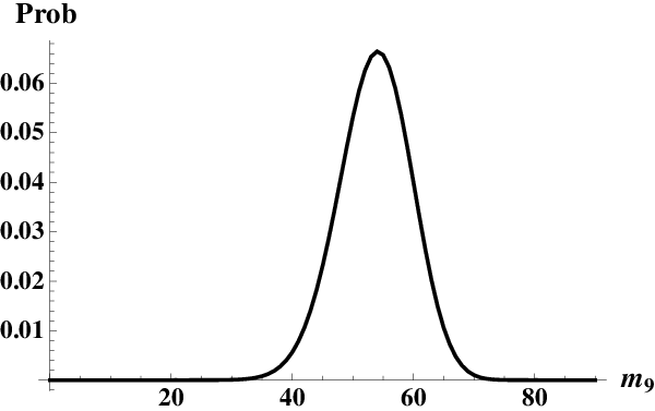
Fig. 9 shows a plot of of Eq. (61) for a set of variables having a large value of . To get this plot we used . We find the exact result compared to the approximation of 54 given by Eq. (33).
Appendix C: Circuit Efficiency comparisons
It is likely, in any set of experimental runs, that a random assortment of values of , and will be averaged over in making a NOON state. What percentage of the inputs will result in good NOON states? Here we compare the corrected and uncorrected efficiencies to get an idea of how successful is the correction circuit in providing good NOON states.
VIII.1 Uncorrected Circuit
With the uncorrected circuit one can, for a given value, compute in the 2D space of , the various possible NOON output numbers, , and the corresponding NOON quality factor and total absolute probability (probability normalized over all five variables) of getting each result. In a 2D plot of the probability one finds the highest factors along , as expected. This line of high is a minimum of absolute probability – nonequal values are more probable. A sample is shown in Fig. 10 for and Note that only the middle seven values give a quality factor greater than 0.90 and only the middle three are greater than 0.95. When is larger, the quality factors drop so that for, say, only the case gives and only the middle three points have . As decreases, the distribution of high quality factors broadens greatly, but one is then getting fewer NOON particles as output, and the absolute probability of occurrence of these states is lower.


We can average the data of Fig. 10 over all to get a NOON that would occur if we accepted all events at constant The result is shown in Fig. 11. The resulting quality factor is low (0.26) because we have averaged over some very poor states. The total probability of getting any results corresponding to is 0.0036.

We can assume that someone using the uncorrected circuit would be more selective and keep only data associated with values that have higher quality factors and sufficiently large values. Thus if one demands that the NOON output particle number be 20 or larger (still for ) for , one will get this 6.2% of the time. Table 2 shows the percentages for various output minimum numbers.
| % () | %() | |
|---|---|---|
| 35 | 0.30 | 0 |
| 30 | 2.7 | 0.2 |
| 20 | 6.2 | 1.6 |
| 15 | 6.2 | 2.0 |
VIII.2 Corrected Circuit
In the corrected circuit we have one more variable , making it very difficult to get the data set equivalent to that which led to, say, Table 2. However, we can analyze a particular case corresponding to fixed values of and output number . We again choose and First we present a NOON that is a probability-weighted average over all and corresponding to those values. Of course, we have determined for each set of the variables and Thus we have a double sum with the probability distribution given by
| (62) |
where and the factor of 2 in the second term takes account of the symmetry that occurs when and are interchanged. The NOON state produced by this process is shown in Fig. 12.

The efficiency in getting this high quality result () is good; that is, output corresponding to any element with this output number occurs with absolute probability 2.1%. This NOON quality comes without any selection of specially chosen values of and as occurred in Table 1. The point is that the probability distribution is small away from the high quality points because the transmission coefficient has been chosen properly.
We can see how the probability distribution selects high quality by taking apart the above NOON output. An important aspect of this is the position in space for which the actual value of is equal to its most likely value, given by Eq. (33). This is the position in the space where the absolute probability will be the largest. Moreover, we expect that the quality factor will be largest here too. Fig. 13 shows the plot of the points where this match of the real agrees with its most probable value.

Suppose we now pick a value of and plot the quality factor and probablity versus : Fig. 14 shows these for There are two peaks in the quality factor corresponding to where crosses the places of maximum probability seen in Figure 13. The cusp occurs at the point where one switches from having to the inverse. The probability shows only the peak at the second crossing; there is also a peak at the first crossing, but it is too small to appear on the graph.


Other samples of such plots show the probability similarly peaking at the point of largest quality factor.
Finally we plot in Fig. 15 the quality factor and probablity, summed over all , as a function of , again for fixed . There are two peaks in the probability since, according to Fig. 13, there are equal probability regions in the space symmetrically at and


Clearly the correction process is successful in producing good quality NOON states with high probability.
References
- [1] J. P. Dowling, Contemp. Phys. 49, 125 (2008).
- [2] A. J. Leggett, Prog. Theor. Phys. Suppl. 69, 80 (1980); J. Phys. Condens. Matter 14, R415 (2002); Phys. Scr. T102, 69 (2002).
- [3] D. M. Greenberger, M. A. Horne, A. Shimony, and A. Zeilinger, Am. J. Phys. 58, 1131 (1990).
- [4] N. D. Mermin, Phys. Rev. Lett. 65, 1838 (1990).
- [5] C. F. Wildfeuer, A. P. Lund, and J. P. Dowling, Phys. Rev. A 76, 052101 (2007).
- [6] J. J . Bollinger, Wayne M. Itano, and D. J. Wineland, Phys. Rev. A 54, R4649 (1996); R. A. Campos, C. C. Gerry, and A. Benmoussa, Phys. Rev. A 68, 023810 (2003).
- [7] A. N. Boto, P. Kok, D. S. Abrams, S. L. Braunstein, C. P. Williams, and J. P. Dowling, Phys. Rev. Lett. 85, 2733 (2000); H. Cable, R. Vyas, S. Singh, and J. P. Dowling New J. Phys. 11, 113055 (2009).
- [8] M. W. Mitchell, J. S. Lundeen, and A. M. Steinberg, Nature 429, 161 (2004).
- [9] J. A. Jones, S. D. Karlen, J. Fitzsimons, A. Ardavan, S. C. Benjamin, G. Andrew, D. Briggs, and J. J. L. Morton, Science 324, 1166 (2009).
- [10] I. Afek, O. Ambar, Y. Silberberg, Science 328, 879 (2010).
- [11] P. Walther, J.-W. Pan, M. Aspelmeyer, R. Ursin, S. Gasparoni, and A. Zeilinger, Nature 429, 158 (2004).
- [12] T. Nagata, R. Okamoto, J. L. O’Brien, K. Sasaki, S. Takeuchi, Science 316, 726 (2007).
- [13] C. K. Hong, Z. Y. Ou, and L. Mandel, Phys. Rev. Lett. 59, 2044 (1987).
- [14] H. Cable and J. P. Dowling, Phys. Rev. Lett. 99, 163604 (2007).
- [15] W. J. Mullin and F. Laloë, J. Low Temp. Phys. 162, 250 (2011).
- [16] V. Giovannetti, S. Lloyd, L. Maccone, arXiv:1102.2318v1.
- [17] G. A. Durkin and J. P. Dowling, Phys. Rev. Lett. 99, 070801 (2007).
- [18] M. J. Holland and K. Burnett, Phys. Rev. Lett. 71, 1355 (1993).
- [19] S. L. Braunstein, C. M. Caves, and G. J. Milburn, Ann. Phys. 247, 135 (1996).
- [20] H. F. Hofmann, Phys. Rev. A 79, 033822 (2009).
- [21] G. A. Durkin, New J. Phys. 12, 023010 (2010).
- [22] W. J. Mullin and F. Laloë, Phys. Rev. Lett. 104, 150401 (2010).
- [23] A. J. Leggett and A. Garg , Phys. Rev. Lett. 54, 857 (1985).
- [24] Y.-J. Wang, D. Z. Anderson, V. M. Bright, E. A. Cornell, Q. Diot, T. Kishimoto, M. Prentiss, R. A. Saravanan, S. R. Segal, and S. Wu, Phys. Rev. Lett. 94, 090405 (2005).
- [25] W. S. Bakr, J. I. Gillen, A. Peng, S. Fölling, and M. Greiner, Nature 462, 74 (2009).
- [26] D. Rosenberg, A. E. Lita, A. J. Miller, and S. W. Nam, Phys. Rev. A 71, 061803(R) (2005)
- [27] R. Prevedel, P. Walther, F. Tiefenbacher, P. Böhi, Rainer Kaltenbaek, T. Jennewein, and A. Zeilinger, Nature 445, 65 (2007).
- [28] X. Chen and L. Jiang, J., Phys. B At. Mol. Opt.Phys. 40, 2799 (2007).