Violation of the area law and long range correlations in infinite matrix product states

In general, one can write the state of a one-dimensional chain of $N$ spins as

where $s_{i}$ is summed over all possible states of the $i$th spin and $\psi(s_{1},\ldots,s_{N})$ are complex coefficients. We shall here assume $s_{i}=\pm 1$. For the family of states investigated in the present work, $\psi(s_{1},\ldots,s_{N})$ is chosen as

where

and we shall always take $N$ to be even. Here, $\delta$ is either $0$ or $1$, $\alpha$ is a real and positive parameter, $z_{n}$ is a complex parameter, $\phi_{0}$, $\pi_{0}$, and $a_{m}$ are operators for which the nonvanishing commutation relations are $[\phi_{0},\pi_{0}]=i$ and $[a_{n},a_{m}^{\dagger}]=\delta_{nm}$, the expectation value in (3) is evaluated with respect to the state $|0\rangle$ defined by $\pi_{0}|0\rangle=a_{m}|0\rangle=0$, and we note that the resulting state is not necessarily normalized. Graphical illustrations of the MPS and iMPS constructions are given in Fig. 1.

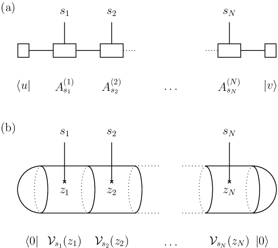
In the limit $M\rightarrow\infty$ and $\delta=1$, (4) is a chiral vertex operator of a conformal field theory with central charge $c=1$ [11] as investigated in [10]. In the following, we shall refer to the mode on which $\phi_{0}$ and $\pi_{0}$ act as the zero mode and use the term $m$th mode for the mode on which the bosonic annihilation operator $a_{m}$ acts. Note that $\delta=1$ ($\delta=0$) corresponds to keeping (omitting) the zero mode. We consider both cases because the zero mode has a special status and because we are particularly interested in the simplest situation $\delta=0$ and $M=1$, which involves only one mode.

Evaluating the expectation values, we find the explicit form

where $\delta_{s}$ is defined to be unity if $\sum_{n=1}^{N}s_{n}=0$ and zero otherwise. Note that the first factor in square brackets is the contribution from the zero mode, while the exponential is a product of $M$ factors coming from modes $1$ to $M$. In this and the next section, we choose $z_{n}=\exp(2\pi in/N)$, which gives a translationally invariant state for $\delta=0$. (Note that the definition in (3) does not impose $|\psi\rangle$ to be translationally invariant in general.)

To investigate the properties of the state (5), we first compute the Renyi entropy $S_{L}^{(2)}=-\log[\Tr(\rho_{L}^{2})]$, where $\rho_{L}$ is the reduced density operator obtained by tracing out spins $L+1$ to $N$. A small calculation shows that

where the stars mean complex conjugation. The right hand side of this equation has the form of an expectation value, and we compute it numerically by using the Metropolis Monte Carlo algorithm [15].

For an MPS, the entropy of a subchain of length $L$ is limited by the logarithm of the virtual dimension, which is independent of $L$, and for critical systems the entropy grows approximately as $\ln(L)$ when the length of the subchain is short compared to the length of the complete chain [10]. The results for the state (5) given in Fig. 2 shows that the entropy increases significantly, when the vertex operators are truncated to a finite number of modes. This is a bit surprising because we go from infinitely many modes representing infinite dimensional Hilbert spaces to a finite number of modes representing infinite dimensional Hilbert spaces and shows that a single bosonic mode is, in fact, sufficient to obtain states, which contain a significant amount of entropy. We also observe that qualitatively similar results are obtained if the zero mode is or is not included.

In addition to the pictorial representation of the transition from $M=1$ to $M\rightarrow\infty$ in Fig. 2(a), it is interesting to investigate the approximate scaling behavior of $S_{L}^{(2)}$ with $L$ as a function of $M$. Inspired by the critical case $M\rightarrow\infty$, for which the entropy is expected to follow the relation $S_{L}^{(2)}=\ln(N\sin(\pi L/N)/\pi)/4+\textrm{constant}$ [10], we plot the entropy as a function of $\sin(\pi L/N)$ in Fig. 3. For each value of $M$ we fit a power law of the form $S_{L}^{(2)}=a(\sin(\pi L/N))^{b}+c$ to the data, where $a$, $b$, and $c$ are fitting parameters, and we plot the exponent $b$ as a function of $M$. The fits show that the power law is a good approximation when $M$ is small provided the subchain does not consist of only a few spins. For intermediate $M$’s there are some discrepancies, and for $M=50$ and $M\rightarrow\infty$, the exponent is close to zero. This reflects the transition to a logarithmic scaling for $M\rightarrow\infty$. Specifically, we find that $S_{L}^{(2)}=0.246\ln(\sin(\pi L/N))+2.39$ provides a good fit to the data for $M\rightarrow\infty$, which is in accordance with the expression given above. Figure 4 provides a schematic summary of the scaling behavior of the entropy for MPS, the critical iMPS studied in [10], and the iMPS considered in the present article.

The dependence of the entropy on $\alpha$ is exemplified in Fig. 5 for $M=1$ and $\delta=0$, where the entropy is observed to increase with $\alpha$, and a very similar behavior is found for $M=1$ and $\delta=1$. We can hence use $\alpha$ to fine-tune the entropy to a desired value. In Appendices A and B, we show that the entropy for $M=1$ and $\delta=0$ is given approximately by the relation

in the limit of large $N$, where $M_{1}$, $M_{2}$, and $M_{3}$ are the eight-by-eight matrices defined in Eqs. (39), (40), and (41). To obtain this result, we use that $z_{n}=\exp(2\pi in/N)$ has practically the same value for several nearby values of $n$ when $N$ is large and that the sum of $s_{n}$ for such a group of $n$-values approximately follow a Gaussian probability distribution when spin configurations are chosen at random. The expression (7) is also plotted in the figure, and we observe an excellent agreement with the numerical results.

Another important characteristic is the behavior of the correlation function between two operators acting on different spins. Specifically, we shall consider

where $\sigma_{z}(k)$ is the third of the Pauli operators acting on the $k$th spin, $\sigma_{z}(0)=\sigma_{z}(N)$, and the expectation value is computed with respect to the atomic state (5). Note that $|\psi(s_{1},\ldots,s_{N})|^{2}$ is translationally invariant, and hence $\langle\sigma_{z}(n)\sigma_{z}(n+k)\rangle=\langle\sigma_{z}(0)\sigma_{z}(k)\rangle$, where $n$ is an integer, and the argument of $\sigma_{z}$ is understood to be modulus $N$.

Numerical results for the correlation function are given in Fig. 6 for various values of $M$, and we observe an excellent agreement with the approximate relation (for $k\neq N$ modulus $N$) obtained in App. D

which is expected to be valid for $M\ll N$. It is interesting to note that the correlation function for $M=1$ does not decay with the separation $k$ for fixed $N$, but instead exhibits an oscillatory behavior with a wavelength, which is equal to the length of the chain. This is a very different behavior from the critical case $M\rightarrow\infty$ and $\delta=1$, in which the correlation function shows an antiferromagnetic ordering and a magnitude decreasing with $k$ [10]. It is also in contrast to MPS, for which the correlation function decays exponentially with the separation [1]. We also note that the correlation functions for $\delta=1$ and $\delta=0$ only differ by the constant term $-\delta/N$, and both correlation functions do not depend on $\alpha$.

The considered class of states is also interesting from the point of view that the structure of Eq. (3) and the fact that $\mathcal{V}_{s_{n}}(z_{n})$ only depends on the state of the $n$th spin provide a direct recipe for preparing the states experimentally in which an ancilla system sequentially interacts once with each of the spins. The form of the truncated vertex operators furthermore allows us to decompose the ancilla system into $M+\delta$ independent bosonic modes that can be treated separately. Specifically, (3) and (4) imply

where $\prod_{n=1}^{N}o_{n}$ for some set of operators $o_{n}$ is understood to mean $o_{1}o_{2}\ldots o_{N}$, and it is hence possible to prepare the desired state from a simple initial state if one can implement the $M+\delta$ operators in (10).

Let us first consider the operator coming from the $m$th mode. This operator is proportional to

which for $z_{n}=\exp(2\pi in/N)$ is the expectation value of a product of $N$ displacement operators, where the displacement $\sigma_{z}(n)\sqrt{\alpha}m^{-1/2}\exp(2\pi inm/N)$ accomplished by the $n$th displacement operator depends on the state of the $n$th spin. In other words, we can implement the contribution from the $m$th mode by initializing the bosonic mode in the vacuum state, engineering the Hamiltonian

where $g$ is a coupling strength, applying it for a time $t$ such that $\int_{0}^{t}gdt=\sqrt{\alpha}m^{-1/2}\exp(2\pi inm/N)$ for each of the spins, and finally projecting the bosonic mode on the vacuum state via a conditional measurement.

The bosonic mode could be a single mode of a cavity, and the spins could be atoms traversing the cavity one by one as illustrated in Fig. 7. The movements of the atoms in and out of the cavity could, for instance, be accomplished by the method demonstrated in [16], where laser fields are used to form a conveyor belt for the atoms. The two levels of the spins correspond to two ground state levels $|{\pm 1}\rangle$ of the atoms, and we assume that the cavity field couples only the state $|{+1}\rangle$ to an excited state. By choosing the cavity field to be far detuned from the atomic transition and driving the same transition with a classical field at the same frequency, one achieves the Hamiltonian

where $\Delta$ is the detuning between the atomic transition and the frequency of the cavity mode, $\tilde{g}$ is the coupling strength between the cavity mode and the atom, and $\Omega$ is the Rabi frequency for the driving of the atom with the classical field. The ac stark shift $-\hbar|\Omega|^{2}|{+1}\rangle\langle{+1}|/\Delta$ can be compensated by coupling $|{+1}\rangle$ to another excited state with another classical field, and the term $-\hbar|\tilde{g}|^{2}a_{m}^{\dagger}a_{m}|{+1}\rangle\langle{+1}|/\Delta$ can be neglected if $\Omega$ is sufficiently large. The resulting interaction only displaces the amplitude of the cavity field if the atom is in the state $|{+1}\rangle$. One way to correct for this is to apply a displacement operation to the cavity field, which is independent of the state of the atom. This is, in fact, not necessary, however, because the error in the displacement occurring when the $n$th atom interacts with the cavity field is opposite to the error in the displacement occurring when the $(n+N/2)$th atom interacts with the cavity field. Except for an overall phase factor, the only consequence of not applying the additional displacement operations is to introduce some single atom phase factors, but these can be canceled by applying the unitary operator

to the atoms after all the interactions with the cavity field have taken place. The final projection of the cavity field on the vacuum state may, for instance, be accomplished with a photo detector, or one can use atoms to probe the state of the cavity field (see [17] for an implementation in the microwave regime).

The contribution from the zero mode (if it is included) can be implemented along similar lines. The key point is to note that

where $a_{0}$ is a bosonic annihilation operator and the expectation value is evaluated in the vacuum state of that operator. We can hence use the same procedure as before if we take the limit where $|{\int\tilde{g}\Omega dt}|$ goes to infinity while the deviation of the phase of $\int\tilde{g}\Omega dt$ from $-\pi/2$ goes to zero as $1/|{\int\tilde{g}\Omega dt}|^{2}$. The physical reason why a $\delta_{s}$ appears in this limit is that the norm of the sum of the displacements is either zero or infinite when the amplitude of the classical field is infinite, and there is only a nonvanishing overlap with the vacuum state of the cavity mode after the interactions in the former case.

We finally need a way to initialize the atoms in the state $\sum_{s_{1},\ldots,s_{N}}|s_{1},\ldots,s_{N}\rangle$. This can be done by pumping all the atoms to the state $|{-1}\rangle$ and applying a $\pi/2$ pulse between the levels $|{-1}\rangle$ and $|{+1}\rangle$.

The proposed generation scheme is only efficient if the probability $P_{M}$ for successfully projecting all the cavity modes on the vacuum state after the interactions with the atoms is not too small. $P_{M}$ is the square of the norm of the final state of the atoms relative to the square of the norm of the initial state of the atoms, and we find

where

We evaluate the expression in (16) numerically by including a larger and larger number of randomly chosen configurations of the spins in the sum until the sum divided by the number of included configurations converges to a constant value, and the results are shown in Fig. 8.

It is possible to obtain an analytical approximation to $P_{M}$ as follows. In App. A we show that the values of $x_{N}=N\Real(\tilde{s}_{1})$ and $y_{N}=N\Imag(\tilde{s}_{1})$ for randomly chosen spin configurations in the limit of large $N$ follow a Gaussian probability distribution

and the same distribution also applies to the real and imaginary parts of $N\tilde{s}_{q}$. Hence, if we start from the atomic state $\sum_{s_{1},\ldots,s_{N}}|s_{1},\ldots,s_{N}\rangle$ and only apply the operations required to take the $q$th mode in the truncated vertex operators into account, the projection on the vacuum state for that mode proceeds successfully with probability

Since the inclusion of the zero mode projects the atomic state on the subspace of states with $\sum_{n=1}^{N}s_{n}=0$ in addition to introducing some phase factors, the probability of success when we only include the zero mode is $2^{-N}\times N!/[(N/2)!]^{2}$, which by use of Stirling’s approximation can be replaced by $[2/(\pi N)]^{1/2}$ for large $N$.

From the arguments in App. C we expect the distributions of $N\tilde{s}_{q}$ for a moderate number of different values of $q$ to be approximately independent in the limit of large $N$. This means that the success probability $P_{M}$ factorizes into a product of the individual contributions from the $M+\delta$ modes, and we hence predict the approximate relation

This result is also plotted in Fig. 8, and we see an excellent agreement with the numerical computations even for only moderately high $N$. Equation (20) suggests that $P_{M}$ scales approximately as $N^{-(M+\delta/2)}$, and for moderate $M$ we hence conclude that the number of operations required to prepare the desired state grows only polynomially in $N$. The proposed method can, however, not be used for generating the critical state investigated in [10] since the success probability vanishes in the limit $M\rightarrow\infty$.

One way to modify the preparation scheme is to modify the state of the cavity field before and after the interactions with the atoms. A nontrivial example is to apply a squeezing operation, i.e., the time evolution operator $\exp(r(e^{2i\phi}(a_{1}^{\dagger})^{2}-e^{-2i\phi}a_{1}^{2})/2)$, where $r$ and $\phi$ are real parameters, before the interactions and to apply the inverse operation after the interactions. Physically, this can be done by placing a nonlinear crystal inside the cavity and pumping it with a classical field [18], and mathematically this amounts to replacing the vacuum expectation value in Eq. (3) by an expectation value with respect to the squeezed vacuum state

where $A=e^{2i\phi}\tanh(r)/2$, i.e.,

where $\tilde{s}_{1}$ is defined in Eq. (17) and we have used a theorem derived in [19] to evaluate the expectation value.

We can use the same approach as for $A=0$ to derive analytical approximations to the Renyi entropy (see App. B), the correlation function (see App. D)

(for $k\neq N$ modulus $N$), and the success probability

Numerical and analytical results for the entropy and the correlation function are provided in Figs. 9 and 10, and it is apparent that $|A|$ needs to be close to $1/2$ in order to observe significant deviations from the case $A=0$. More precisely, Eqs. (23) and (24) show that $(1+4|A|^{2})/(1-4|A|^{2})$ should be on the order of $\alpha N$ or larger for the squeezing to have a significant effect. If $|A|$ is close to $1/2$, we observe an increase in the entropy compared to the case $A=0$. The correlation function keeps the same shape but the amplitude decreases from $2/N$ to $1/N$ as $A$ increases from $0$ to $1/2$. Finally, we note that $P_{\textrm{sq}}\sim\sqrt{\epsilon/(\alpha N)}$ when $|A|=1/2-\epsilon$ and $\epsilon\ll 1/(\alpha N)$.

Another natural way to modify the preparation scheme is to allow a bit of the cavity field to leak out between each interaction with one atom and project the field that has escaped from the cavity on the vacuum state to remain within the set of pure states. The leakage corresponds to the application of a beam splitter operation, and hence

where $b_{n}$ are bosonic annihilation operators, i.e., $[b_{n},b_{m}^{\dagger}]=\delta_{nm}$, and $g$ is a parameter quantifying the amount of leakage (the relative loss in intensity is $\sin^{2}(|g|)$). Commuting operators in this expression, one can show that it is again possible to only displace the cavity field each time an atom is in the state $|{+1}\rangle$ provided (i) one applies appropriate displacement operations to the field that leaks out of the cavity, (ii) one applies an appropriate displacement to the cavity field after completing the interaction with all the atoms and before the projection on the vacuum state, and (iii) one applies appropriate single atom phase shifts to the atoms. We note that the displacements of the field amplitudes can be accomplished by use of a strong classical field and a beam splitter as proposed in [20].

Evaluating the expectation value, we find that the wave function

is, in fact, again given by Eq. (5) (with $M=1$ and $\delta=0$), but now $z_{n}=\cos(|g|)^{n}e^{2\pi in/N}$. The numerical results for the entropy and the correlation function (8) in Figs. 11 and 12 show that even a small leakage has a significant impact on the properties of the produced states. The entropy is reduced significantly, and the correlation function now decays with separation. For $g=0.05\times\pi/2$, the decay is roughly exponential. This indicates that it is important to exclude losses from the setup to obtain the high entropies and long range correlations found in Sec. II. The correlation function also shows that antialignment of nearby spins become more favorable when leakage is included. This can be understood from the fact that the field leaking out of the cavity is more likely to be projected on the vacuum state if the total displacement of the cavity field is close to zero at all times during the preparation.

The probability of success

is plotted as a function of the number of spins in Fig. 13. $P_{\textrm{pr}}$ decreases significantly with increasing $|g|$, and for $g=0.05\times\pi/2$, the decrease in $P_{\textrm{pr}}$ with $N$ is almost exponential as detailed in the figure.

References

- [1] J. I. Cirac and F. Verstraete, J. Phys. A: Math. Theor. 42, 504004 (2009).
- [2] M. B. Hastings, J. Stat. Mech., P08024 (2007).
- [3] J. Eisert, M. Cramer, and M. B. Plenio, Rev. Mod. Phys. 82, 277 (2010).
- [4] F. Verstraete and J. I. Cirac, Phys. Rev. B 73, 094423 (2006).
- [5] C. Holzhey, F. Larsen, and F. Wilczek, Nucl. Phys. B 424, 443 (1994).
- [6] P. Calabrese and J. Cardy, J. Stat. Mech. P06002 (2004).
- [7] F. Verstraete and J. I. Cirac, Phys. Rev. B 73, 094423 (2006).
- [8] R. N. C. Pfeifer, G. Evenbly, and G. Vidal, Phys. Rev. A 79, 040301(R) (2009).
- [9] S. Montangero, M. Rizzi, V. Giovannetti, and R. Fazio, Phys. Rev. B 80, 113103 (2009).
- [10] J. I. Cirac and G. Sierra, Phys. Rev. B 81, 104431 (2010).
- [11] P. Di Francesco, P. Mathieu, and D. Sénéchal, Conformal Field Theory, Springer (1997).
- [12] C. Schön, E. Solano, F. Verstraete, J. I. Cirac, and M. M. Wolf, Phys. Rev. Lett. 95, 110503 (2005).
- [13] C. Schön, K. Hammerer, M. M. Wolf, J. I. Cirac, and E. Solano, Phys. Rev. A 75, 032311 (2007).
- [14] T. J. Osborne, J. Eisert, and F. Verstraete, Phys. Rev. Lett. 105, 260401 (2010).
- [15] N. Metropolis, A. W. Rosenbluth, M. N. Rosenbluth, A. H. Teller, and E. Teller, J. Chem. Phys. 21, 1087 (1953).
- [16] K. M. Fortier, S. Y. Kim, M. J. Gibbons, P. Ahmadi, and M. S. Chapman, Phys. Rev. Lett. 98, 233601 (2007).
- [17] C. Guerlin, J. Bernu, S. Deléglise, C. Sayrin, S. Gleyzes, S. Kuhr, M. Brune, J.-M. Raimond, and S. Haroche, Nature 448, 889 (2007).
- [18] R. Loudon, The Quantum Theory of Light, Oxford Science Publications, 3rd edition (2000).
- [19] N. H. McCoy, Proceedings of the Edinburgh Mathematical Society (Series 2), 3, pp 118-127 (1932).
- [20] M. G. A. Paris, Physics Letters A 217, 78 (1996).