Improving Sensitivity to Weak Pulsations with Photon Probability Weighting

M. Kerr Affiliation: Kavli Institute for Particle Astrophysics and Cosmology, Stanford University, 452 Lomita Mall, Stanford, CA 94305, USA Email: kerrm@stanford.edu Alternate Affiliation: Einstein Fellow

Abstract

All $\gamma$ -ray telescopes suffer from source confusion due to their inability to focus incident high-energy radiation, and the resulting background contamination can obscure the periodic emission from faint pulsars. In the context of the Fermi Large Area Telescope, we outline enhanced statistical tests for pulsation in which each photon is weighted by its probability to have originated from the candidate pulsar. The probabilities are calculated using the instrument response function and a full spectral model, enabling powerful background rejection. With Monte Carlo methods, we demonstrate that the new tests increase the sensitivity to pulsars by more than $50\%$ under a wide range of conditions. This improvement may appreciably increase the completeness of the sample of radio-loud $\gamma$ -ray pulsars. Finally, we derive the asymptotic null distribution for the $H$ -test, expanding its domain of validity to arbitrarily complex light curves.

Subject headings

methods: statistical — methods: data analysis — pulsars: general — gamma rays: general

I. Introduction

Though the detection and characterization of periodic emission from neutron stars has historically been the province of radio astronomers [23, 11, 25, e.g.], increasingly sensitive instruments have enabled the study of pulsars at high energy. Neutron stars accreting near their Eddington limit were detected in X-rays as accretion-powered pulsars [37] in the 1970s by UHURU [22], while the sensitive ROSAT and ASCA missions detected faint magnetospheric emission from a population of rotation-powered X-ray pulsars [12].

At even higher energies, the handful of well-known $\gamma$ -ray pulsars—e.g., Vela [34] and Geminga [14]—have been joined by a host of new pulsars detected by the Fermi Large Area Telescope (Fermi-LAT). While the superb sensitivity of Fermi-LAT has facilitated the first discoveries of pulsars in $\gamma$ rays alone [1, 3], a foundation of pulsar science with Fermi-LAT is the extensive support from the radio community. E.g., the Pulsar Timing Consortium [33] generates timing solutions for over 200 pulsars with high spindown luminosity, $\dot{E}>10^{34}$ erg s^-1. These timing solutions enable the long integrations necessary to detect periodicity in sparse Fermi-LAT photons, and so far more than 30 timed pulsars have been detected in $\gamma$ rays [5, 8, 2, e.g.].

Although the precise emission geometry of pulsars is still unknown, it is not unreasonable to believe that $\approx 50\%$ of radio-loud pulsars are also $\gamma$ -ray loud [32], a fraction that may be even larger for millisecond pulsars. If this is indeed the case, then many of the luminous radio-timed pulsars are visible in $\gamma$ rays but below the current sensitivity of the LAT. While Fermi-LAT continuously observes the GeV sky, the flux above which pulsars are detectable only decreases as $t^{-1/2}$ . Ten years of observation will only decrease the current flux threshold by a factor of $\sim$ 2.

Improved analysis techniques can beat this rate, and in this vein we outline better statistics for testing for periodicity. To date, such tests [8] have used only the arrival time/phase of a photon. As shown by Bickel et al. [15, hereafter BKR08], the additional data available—the photon’s reconstructed energy and position—allow the calculation of a probability that the given photon originated from the candidate pulsar, and that incorporating this probability into the test statistics helps reject background and increase the sensitivity to pulsations. Although we focus on the application of the technique to LAT data, we note that the scheme is applicable to any photon-counting instrument in which sources are not perfectly separated from their background, e.g. searches for X-ray pulsation in observations of a pulsar embedded in a pulsar wind nebula.

The paper is organized as follows. We begin in Section II by giving an overview of a family of statistics—based on trigonometric moments and formulated as a score test for pulsation—that includes the weighted pulsation tests discussed here. In Sections II.1, we review the $Z^{2}_{m}$ and $H$ -test statistics and define modified versions incorporating weights. We outline the calculation of probability weights appropriate for the LAT in Section III and in Section IV we demonstrate the superior performance of the weighted versions of the $Z^{2}_{m}$ and $H$ -test statistics. In the Appendix, we derive the asymptotic calibration for the $H$ -test, a new result expanding the scope of the test.

II. Statistical Tests for Periodicity

A timing solution (ephemeris) defines a map from photon arrival time $t$ to phase $\phi$ , e.g. neutron star rotational phase. The flux from a pulsar can be written as

f(\phi,E)\propto 1+\eta\,\sum\limits_{k=1}^{\infty}\alpha_{k}\cos(2\pi k\phi)+\beta_{k}\sin(2\pi k\phi).

(1)

For simplicity, we have assumed the pulsar spectrum is independent of phase.

The null hypothesis—no pulsation—is given by $\eta=0$ . By considering the likelihood for photon arrival times, BKR08 derived a test statistic¹¹ 1 The form of the statistic presented here requires that the pulsar period be short relative to the timescale on which the detector response changes. This is so for the Fermi-LAT. for $\eta>0$ ,

Q\equiv\frac{2}{T}\sum_{k=1}^{\infty}(\alpha_{k}\,\hat{\alpha}_{k})^{2}+(\beta_{k}\,\hat{\beta}_{k})^{2},

(2)

where $T$ is the total integration time and

\hat{\alpha}_{k}=\sum_{i=1}^{n}w_{i}\,\cos(2\pi k\phi_{i});\ \ \hat{\beta}_{k}=\sum_{i=1}^{n}w_{i}\,\sin(2\pi k\phi_{i}),

(3)

where the sum is over the list of $n$ photons and $w_{i}$ is some weight. (See Eq. 17 of BKR08, from which this form is adapted.) For $w_{i}=1/n$ , these are estimators of the trigonometric moments of the distribution and Monte Carlo estimators for the coefficients of the Fourier transform. If $w_{i}$ is the probability that a photon comes from the pulsar, the weights are optimal in the sense that $Q$ is a score test, which is locally most powerful. Moreover, the statistic is manifestly invariant under phase shifts $\phi\rightarrow\phi+\delta\phi$ . (See also the result of Beran [13], who considered a similar class of statistics.) From Central Limit Theorem arguments, BKR08 show that for a finite collection of $m$ harmonics, $Q$ has an asymptotic distribution of $\chi^{2}_{2m}$ .

II.1. The $Z^{2}_{m}$ Test

A simple realization of such a statistic, with $w_{i}=1$ and $\alpha_{k}=\beta_{k}=1$ for $k\leq m$ and $\alpha_{k}=\beta_{k}=0$ for $k>m$ , known as the $Z^{2}_{m}$ statistic,

Z^{2}_{m}=\frac{2}{n}\sum_{k=1}^{m}\hat{\alpha}_{k}^{2}+\hat{\beta}_{k}^{2},

(4)

has been a workhorse for searches for $\gamma$ -ray pulsars. (Note the change in normalization: $1/T\approx 1/n$ .) A $Z^{2}_{2}$ test was used in a search for pulsations in COS-B data using timing solutions for $145$ radio pulsars [17]. A similar search of EGRET data [29] used $Z^{2}_{m}$ tests with 1, 2, and 10 harmonics, the $H$ -test (see below), and the “ $Z^{2}_{2+4}$ ” test which is defined as above but with summation restricted to the 2nd and 4th harmonics. $Z^{2}_{m}$ forms an integral part of the $H$ -test, and continues to see use in analysis of Fermi-LAT data [8].

From the discussion above, we expect $Z^{2}_{m}$ to be distributed as $\chi^{2}_{2m}$ in the null case, but this result holds if and only if the $\hat{\alpha}_{k}$ and $\hat{\beta}_{k}$ coefficients are statistically independent. However, in some cases they may be highly dependent. For a single observation, $\alpha_{k}$ ( $\beta_{k}$ ) can be inverted to find the original rv, $\phi$ , and thus all coefficients are algebraically determined. For large samples from a uniform distribution, however, a given coefficient conveys little information about the underlying $\{\phi_{i}\}$ and the coefficients are approximately independent. Although the requirement on the detector response assures uniformity, if the null distribution is peaked, the coefficients remain correlated for arbitrarily large sample sizes.

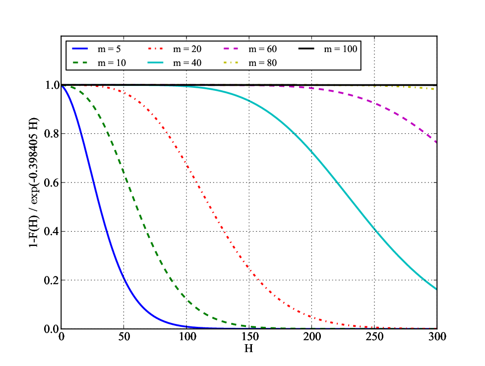
To determine the minimum sample size required to reach the asymptotic $\chi^{2}$ distribution, we performed a Monte Carlo study of the convergence as a function of both sample size and maximum harmonic ( $m$ ), shown in Figure 1. Evidently, a sample size of at least $50$ phases is required for robust significance estimation at the $3\sigma$ level, and convergence appears to improve for higher values of $m$ .

Refer to caption — Figure 1.— The observed distribution for the $Z^{2}_{m}$ statistic for varying sample size and maximum harmonic ( $m$ ). The asymptotic calibration is shown as a solid line, while the solid band gives the empirical distribution function of the Monte Carlo realizations. The width indicates the statistical uncertainty estimated as $\sqrt{N(>=TS)}$ .

The defintion of the $Z^{2}_{m}$ can be viewed as a set of hard cuts for which $w_{i}=1$ for some set of photons and $w_{i}=0$ for all other photons. By allowing arbitrary values for $w_{i}$ we implement soft cuts in which we ideally assign higher (lower) weights to photon associated with the pulsar (background). We thus define the weighted $Z^{2}_{m}$ as

Z^{2}_{2mw}\equiv\frac{2}{n}\,\left(\frac{1}{n}\sum\limits_{i=1}^{n}{w_{i}^{2}}\right)^{-1}\sum_{k=1}^{m}\hat{\alpha}_{k}^{2}+\hat{\beta}_{k}^{2}.

(5)

As a realization of the test statistic of Eq. 2, its calibration remains $\chi^{2}_{2m}$ . Again, note the expression of the normalization in terms of the data; the relation can be seen in terms of a random walk.

II.2. The $H$ -Test

It is clear from Eq. 2 that for an optimal test, the empirical coefficients should be weighted by the true Fourier coefficients, which are a priori unknown. The estimation of unit coefficients up to a maximum harmonic $m$ in the $Z^{2}_{m}$ is crude, and choosing $m$ too small will result in a loss of power against sharply-peaked light curves, while $m$ too large will lose power against broad, sinusoidal light curves. To improve on this, de Jager et al. [21] proposed the $H$ -test, which estimates $m$ from the data. They defined

H_{m}=\max\left[Z^{2}_{i}-c\times(i-1)\right],1\leq i\leq m

(6)

and specifically recommended $m=20$ and $c=4$ as an omnibus test. They provided a Monte Carlo calibration of the tail probability and, in a recent paper [20] provide an estimate $1-F_{H_{20}}(h)\approx\exp(-0.4\times h)$ good to $h\approx 70$ . We derive the analytic, asymptotic calibration for all values of $m$ , $c$ , and $h$ in the Appendix and use this calibration anywhere a conversion from $h$ to chance of Type I error (i.e., “ $\sigma$ ”) is needed.

This calibration depends only on the asymptotic $\chi^{2}_{2m}$ calibration of $Z^{2}_{m}$ , and so it also holds for $Z^{2}_{mw}$ and thus for a weighted H-test statistic

H_{mw}\equiv\max\left[Z^{2}_{iw}-c\times(i-1)\right],1\leq i\leq m.

(7)

We adopt the original values $m=20$ and $c=4$ below.

III. Calculating Photon Probabilities

The optimal choice of weight is the probability that a photon originates from the pulsar, and we outline the calculation of this quantity for the Fermi-LAT. We have available three pieces of information, viz. the photon’s reconstructed energy, position, and arrival time. For pulsars, the arrival time is necessary for computation of the phase but can otherwise be ignored except in rare cases, e.g. a candidate near a bright, highly variable blazar. We thus consider time-averaged quantities only. (Recall we have assumed phase-independent pulsar spectra. Spectra generally are dependent on phase [9, e.g.], but such using a phase-averaged spectrum incurs little error.)

Probabilities constructed using only the photon position have been employed profitably for COS-B and EGRET analyses [16, 31, 27]. This approach has the advantage of requiring no knowledge of source spectra and works well for a detector with an excellent and/or energy-independent psf. The Fermi-LAT, on the other hand, has a comparatively poor psf that varies by more than two orders of magnitude between $100$ MeV and $100$ GeV [10]. A typical source will have many background photons within the psf radius at low energy but very few at high energies, and a probability based solely on position cannot discriminate against the many low energy background photons.

We address the strong dependence of S/N on energy by including the estimated photon energy in the probability calculation. Briefly, a point source is characterized by its photon flux density (ph cm^-2 s^-1 MeV^-1) which we model as $\mathcal{F}(E,\vec{\lambda})$ , with $E$ the energy and $\vec{\lambda}$ some set of parameters (e.g., the normalization and photon index for a power law; these parameters will typically be estimated via maximum likelihood analysis as discussed in the following section). We assume the source is stationary. If the exposure²² 2 The exposure calculation for the Fermi-LAT involves summing the detector response over the pointing history of the spacecraft. to the position of the source, $\vec{\Omega}_{0}$ , is given by $\epsilon(E,\vec{\Omega}_{0})$ (cm² s), then the expected differential rate (ph MeV^-1 sr^-1) in the detector from the $j$ th source is

r_{j}(E,\vec{\Omega})=\mathcal{F}(E,\vec{\lambda})\,\epsilon(E,\vec{\Omega}_{0})\,f_{\mathrm{psf}}(\vec{\Omega};\vec{\Omega}_{0},E),

(8)

where $f_{\mathrm{psf}}(\vec{\Omega};\vec{\Omega}_{0},E)$ denotes the psf of the instrument for the incident energy and position. While the psf only depends on incidence angle, the highly structured diffuse background motivates preservation of the full position.

For a photon observed with energy near $E$ at a position near $\vec{\Omega}$ , the probability that it originated at the $j$ th source is simply

w_{j}(E,\vec{\Omega}|\vec{\lambda})\equiv\frac{r_{j}(E,\vec{\Omega},\vec{\lambda}_{j})}{\sum\limits_{i=1}^{N_{s}}r_{i}(E,\vec{\Omega},\vec{\lambda}_{i})},

(9)

where $N_{s}$ is the number of contributing sources. The weight can approach $1$ for bright pulsars and at high energies, where the LAT psf becomes narrow.

IV. Performance in Fermi-LAT Pulsation Searches

The primary goal in adopting the weighted versions of pulsation test statistics is, of course, to find more genuine pulsars. In statistical language, we want to minimize Type I Error (false positives) and Type II error (false negatives). We address these two in turn by comparing weighted and unweighted versions of the $Z^{2}_{m}$ and H-test statistics. Although BKR08 provide an analytic expression for the increased detection significance offered by photon weights (see Eq. 23 of that work), it is not suitable for determining the global performance improvement since the optimal data selection for the unweighted tests is unknown a priori. We thus assess the performance of the tests on an ensemble of simulated pulsars.

IV.1. Simulation Details

The Fermi-LAT Science Tool³³ 3 http://fermi.gsfc.nasa.gov/ssc/data/analysis/scitools/overview.html gtobssim uses a detailed characterization of the instrument response function to simulate events from modeled point and diffuse sources. We simulate a point source—the candidate pulsar—with a realistic pulsar spectrum,

\frac{dN}{dE}\propto(E/\mathrm{GeV})^{-\Gamma}\exp(-E/E_{c})

(10)

with $\Gamma=1.5$ and $E_{c}=3$ GeV. This spectrum is typical of many pulsars and is approximately that of the middle-aged Vela pulsar [4]. We place the source at (R.A., Decl.) = (128.8463, -45.1735), the position of Vela. For the background, we simulate photons from the two diffuse background models used in the 1FGL catalog analysis [6], gll_iem_v02—a model of the Galactic diffuse background due to cosmic rays—and isotropic_iem_v02—an isotropic background including contributions from unresolved extragalactic point sources and instrumental backgrounds. In all, we simulate one year of integration using the spacecraft pointing history from 2009.

The normalization of Eq. 10 is chosen to yield a bright source with an integral photon flux from 100 MeV to 100 GeV of $\mathcal{F}_{sim}\equiv 10^{-5}$ ph cm^-2 s^-1. We are interested in detection of dim sources, so from this set of photons we select subsets emulating sources with appropriately lower fluxes, e.g. $\mathcal{F}_{tar}=10^{-8}$ ph cm^-2 s^-1, by (a) drawing the target number, $N_{tar}$ , of photons from a Poisson distribution with mean $N_{tot}\times\mathcal{F}_{tar}/\mathcal{F}_{sim}$ and (b) selecting a subset of $N_{tar}$ of the original photon set at random (without replacement). In this way, we can generate ensembles of statistically independent point sources over a range of fluxes from a single Monte Carlo data set. While we use a single realization of the diffuse photons, we effectively generate a new iteration by randomizing these photons in phase for each ensemble member as we discuss below.

To determine the weights (Eq. 9), we employ gtsrcprob. This Science Tool combines the source models (those used to generate the Monte Carlo data) with the instrument response function to determine the observed source rates and hence the weights. These weights are valid for the simulated point source flux $\mathcal{F}_{5}$ , and must be scaled for the dim ensemble members: $w_{tar}^{-1}-1=(w_{sim}^{-1}-1)\times\mathcal{F}_{sim}/\mathcal{F}_{tar}$ .

The Monte Carlo events as generated by gtobssim have no pulsation. During simulation, each photon is “tagged” with an identifier for its originating source. We assign phases from a uniform distribution to the diffuse background, and for the point source we draw phases from an assumed light curve, typically a normalized sum of wrapped Gaussians.

IV.2. Performance: Type 1 Error

Type I error stems from two sources. First, there is the chance of a fluctuation in the test statistic (TS) sufficiently large to pass the established threshold for rejection of the null hypothesis, i.e., claiming detection of a pulsar. As long as we understand the null distribution of the TS, this particular source of error is easy to control: we simply determine in advance our tolerance to false positives and set the TS threshold accordingly. We must be cautious about applying the asymptotic calibration of the null distribution to small sample sizes. For these cases, it is important to verify the chance probability with a Monte Carlo simulation.

A second, more insidious source of error arises from the strong influence of the data selection scheme on the pulsed S/N, this dependence stemming from the energy-dependent psf, source confusion, the strong Galactic diffuse, and the exponential suppression of pulsar emission above a few GeV. To find the best cuts, one is tempted to use the TS itself as a metric, a procedure which invalidates its calibration. Failure to account for this change increases the probability of false positives. Stringent cuts may also make the asymptotic calibration poorer.

Probability-weighted statistics eliminate these problems. Since the weights naturally go to zero for photons with neglible signal, one could in principle include all LAT data in the TS. (In practice, little signal is contained in photons more than $2^{\circ}$ from the source.) Weighting provides an amorphous, optimal selection reflecting, e.g., the proximity of the Galactic plane or the estimated pulsar cutoff energy⁴⁴ 4 In this regard, the weights deliver a data set similar to that proposed by Mayer-Haßelwander & Özel [26], who developed an algorithm for determining an optimal aperture with an arbitrary “edge” determined by the local signal-to-noise ratio. And this single selection incurs no probability of Type I error beyond that due to statistical fluctuations. Finally, the weighted statistic is less susceptible to small-sample effects since all relevant information is included, though for particularly weak signals Monte Carlo validation remains important.

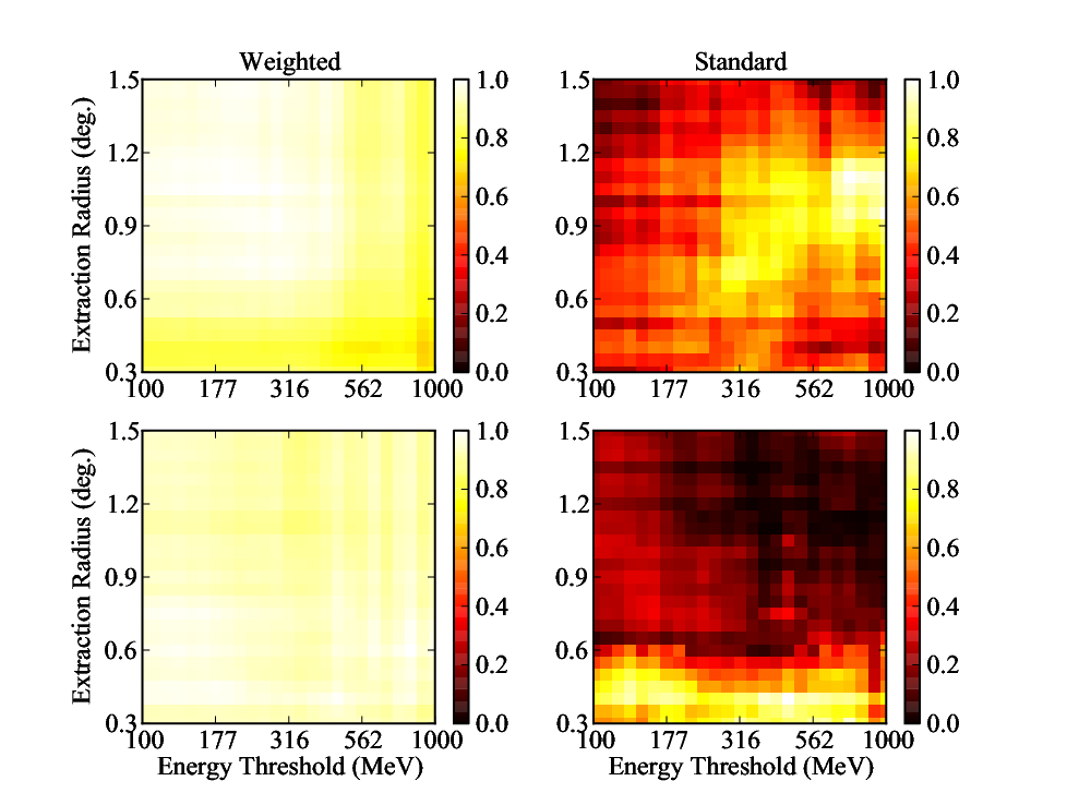
To make these claims concrete, we compare the weighted $H$ -test ( $H_{20w}$ ) and the standard $H$ -test ( $H_{20}$ ) computed over a grid of cuts on photon position and energy (Figure 2). The unweighted statistics show strong TS peaks for certain energy thresholds and extraction radii, and these peaks vary from realization to realization, precluding an a priori calculation of an optimal aperture. The weighted statistics, on the other hand, are largely insensitive to the data selection and perform best for a simple prescription: use as many photons as is practical. We are thus free to use the same loose cuts for all sources, maintaining good performance (peak TS) without the need to tune.

IV.3. Performance: Type II Errors / Sensitivity

We must also consider Type II error—false negatives. In astrophysical terms, this error rate is essentially the sensitivity of the method, i.e., the flux threshold above which a typical source will be significantly detected in a given observation. Indeed, we adopt this approach to define the Type II error. Given a particular light curve, we generate ensembles of sources at a series of increasing fluxes until we identify the flux at which a given fraction of the ensemble has a detection significance above threshold.

More specifically, to compute the detection significance, we calculate the tail probability of the asymptotic distribution for the TS in question convert it to (two-tailed) $\sigma$ units, i.e., a chance probability of $X\sigma$ is $1-(2\pi)^{-1/2}\int_{-X}^{X}dx\,\exp(-x^{2}/2)$ . We determine the flux threshold as that for which $68\%$ of the ensemble deliver a $\sigma$ value above a pre-determined threshold (see below). This is the detection flux threshold. To estimate the $68\%$ level robustly, we fit the ensemble values with a normal distribution and report the appropriate quantile.

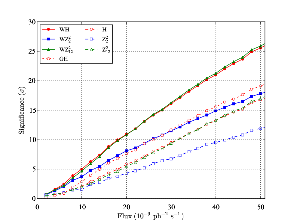
To determine the flux threshold, we need to invert the calculated quantity (tail probability in $\sigma$ units) to the desired quantity (flux threshold). Surprisingly, the relationship between the two is linear. Significance canonically scales as $\sqrt{n}$ , or in this case, since we integrate for exactly one year, $\sqrt{\mathcal{F}}$ . However, here we increase the source flux without increasing the background flux, so we also increase the S/N, and in the background-dominated régime, significance is proportional to the S/N. Thus, $\sigma\propto\mathcal{F}$ , demonstrated in Figure 3.

We choose $4\sigma$ as the threshold which causes us to discard the null hypothesis, i.e., to claim detection of periodic emission. This threshold corresponds to a very small probability of Type I error, about 1 in 15800. Selecting an even higher threshold—and consequently applying the asymptotic calibration well into the distribution’s tails—is not appropriate for these small sample sizes.

To give a modest survey of the statistics outlined above, we present weighted and un-weighted versions of $H_{20}$ , $Z^{2}_{12}$ , and $Z^{2}_{2}$ . Recall that $H_{20}$ is an omnibus test that depends little on light curve morphology, whereas $Z^{2}_{12}$ ( $Z^{2}_{2}$ ) should perform well for light curves with sharp (broad) features. For the unweighted versions of these tests, we select photons with $E>200$ MeV and an angular separation from the candidate $\leq 0.8^{\circ}$ . However, since no single extraction criterion will yield optimal values for the unweighted statistics, we also include a “grid search” for $H_{20}$ . That is, for each source, we extract photons with $E>E_{th}$ and $\theta<\theta_{th}$ , i.e., reconstructed energies above $E_{th}$ and reconstructed positions separated from the true position by less than $\theta_{th}$ . We do this for a grid of $E_{th}$ and $\theta_{th}$ with $E_{th}/\mathrm{MeV}\in(100,178,316,562,1000)$ and $\theta_{th}/\mathrm{deg.}\in(0.5,0.625,0.75,0.875,1.0)$ . We take the maximum resulting test statistic, convert it to chance probability, multiply by 25 (the number of “trials”), and convert this quantity to $\sigma$ units. Finally, for the weighted statistics, we select photons with $E>100$ MeV and $\theta\leq 2^{\circ}$ .

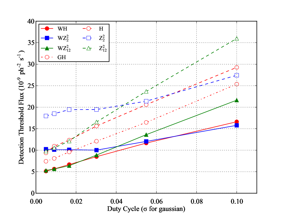
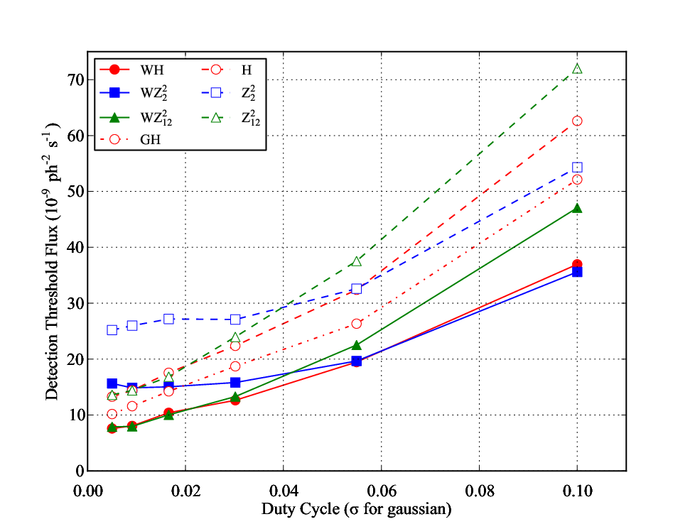
The primary result, shown in Figure 4, shows the flux threshold for each method as a function of “duty cycle”, the fraction of the full phase for which there is appreciable pulsed emission. In this case, the light curves are single Gaussian peaks with a variety of values for their $\sigma$ (standard deviation) parameter; the templates are shown in Figure 5. For a fixed flux, increasing the duty cycle decreases the peak flux, or S/N, and the primary dependence is then an inverse relation between flux threshold and duty cycle. However, there is additional dependence from the nature of each test. It is clear, e.g., that the $H_{20}$ and $Z^{2}_{12}$ perform significantly better than $Z^{2}_{2}$ for low duty cycle sources, while $Z^{2}_{2}$ maintains a slight edge for broad light curves. The $H$ -test does a good job for all duty cycles. More importantly, it is clear that the weighted statistics enjoy a lower threshold for detection—by a factor of 1.5 (grid search) to 2.0 (single cut)— than their unweighted counterparts.

IV.3.1 Two-peaked light curves

Many pulsar light curves display two peaks, often separated by about 0.4-0.5 cycles [8]. We repeat the analysis of the previous section using a template comprising two Gaussian peaks separated by $0.45$ in phase. Real pulsar peaks often have unequal intensities (with an energy-dependent ratio.) We reflect that here with a slightly-dominant leading peak; see Figure 5. As seen in Figure 6, the overall flux thresholds are unsurprisingly increased: at a fixed flux, spreading photons between multiple peaks decreases the overall S/N. The weighted statistics maintain a comfortably decreased flux threshold with respect to the unweighted methods.

IV.3.2 Pulsars with DC Emission Components

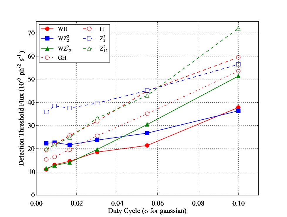
Some pulsars emit an appreciable flux of unpulsed $\gamma$ rays, e.g. PSR J1836+5925 [7]. This steady emission is a confounding factor for the weighted tests, since unpulsed source photons receive the same high probability weights as pulsed photons but are distributed uniformly in phase, decreasing the effective S/N. However, for modest ratios of pulsed to unpulsed flux, the performance of the weighted test is not unduly diminished. In Figure 7, we have examined the flux threshold for a single-peaked light curve with equal contributions of pulsed and unpulsed emission. As expected, we see an overall increased flux threshold of about 2 over the fully-pulsed source (c.f. Figure 4). Despite a slight increase in the ratio of weighted-to-unweighted thresholds, the weighted statistics still offer appreciably improved sensitivity.

IV.3.3 Effect of Uncertainties in Spectral Parameters

From these demonstrations, it is clear that the probability-weighted statistics have, on average, a factor of $1.5$ to $2$ improved sensitivity relative to the unweighted versions. One potential objection is that we have used the known spectra in determining the photon weights, whereas with real data, of course, we must first estimate the spectra of source and background. To assess the impact of using estimated parameters with concomitant uncertainty, we calculate the weights based on parameters estimated via maximum likelihood spectral analysis with the pointlike tool [24].

For this test, we simulated 20 realizations of the Vela-like point source. From Figure 4, we see that the detection threshold is about $\approx 8\times 10^{-9}$ ph cm^-2 s^-1 , and we select this for the ensemble flux. This flux yields about 100 source photons for the 1-year integration period, allowing for asymptotic calibration. Since the background strongly affects the spectral analysis, independent realizations of the diffuse background are important and accordingly we also simulated 20 realizations of the diffuse sources. To the point source data we added phase from a single-Gaussian light curve with $\sigma=0.03$ , while we generated uniform random phases for the diffuse photons.

To assess the impact of uncertain parameters, we first calculate the probability weights using the known model parameters for the pulsar and the diffuse background, i.e., the “ideal” case. We then perform a maximum likelihood spectral fit to estimate the spectral parameters. Since the simulated point source is very dim relative to the background, it is impossible to fit all three parameters. We therefore fix the cutoff energy to $100$ GeV, effectively a power law spectrum. This approach is conservative since we are now using an incorrect spectral model. Using the best-fit values for the flux density and the photon index, we calculate a new set of probability weights. Finally, we compute $H_{20w}$ to determine the significance (a) using the “ideal” weights and (b) using the “measured” weights.

We compare the results for the two cases—in $\sigma$ units—in Figure 8. In general, the detection significance obtained with the “measured” weights is slightly lower than that obtained with the “ideal” weights, although in a few cases statistical fluctuations lead to the opposite outcome. Comparing the population means, the overall significance using measured weights is decreased to $92\%$ of the ideal case, corresponding to an increase in flux threshold of $\sim$ 10%. This effect is small compared to the factor of $1.5-2.0$ increase in flux threshold seen between the weighted and unweighted versions of the $H$ -test. We therefore conclude that—even accounting for uncertainties in the spectral parameters used to calculate the probability weights—weighted statistics offer a significant improvement in sensitivity.

IV.3.4 Comparison of Pulsed and Unpulsed Detection Thresholds

The machinery established above—performing spectral fits on an ensemble to compute the weighted statistics using probabilities estimated from an ML fit—also provides for directly comparing the DC (unpulsed) source significance with the pulsed significance. To estimate the DC significance, we use the result of Chernoff [18] for the asymptotic calibration for the likelihood ratio for a single parameter whose null value lies on a boundary. To apply this calibration, we take the free parameter to be the flux density (which has a boundary at 0) and fix the photon index $\Gamma=2.0$ . The cutoff remains fixed at 100 GeV. With this convention, the DC significance is then given by

\sigma_{DC}=\sqrt{2\times\log\mathcal{L}_{opt}/\mathcal{L}_{0}},

(11)

with $\mathcal{L}_{opt}$ the likelihood value obtained with the best-fit flux density and $\mathcal{L}_{0}$ the likelihood value obtained with the flux density set to zero. It should be noted that $\sigma_{DC}$ is a one-sided significance, so the same value of $\sigma_{DC}$ corresponds to a slightly higher value the “ $\sigma$ ” for the pulsed detection. This discrepancy is small compared to the observed difference in significance.

As in the previous section, we calculate the probability weights using both the Monte Carlo truth values of the parameter and with the best-fit spectrum—in this case, with cutoff energy and photon index fixed—to estimate a pulsed significance with the $H_{20w}$ test.

We compare the unpulsed and pulsed significances in Figure 9. The majority of ensemble members are detected more significantly through pulsations than through unpulsed emission. The measured significance for pulsed detections is a factor of $2.2$ greater than for DC detection. If we assume that the detection flux threshold is linear in $\sigma_{DC}$ as it is in the pulsed significance, this means we require sources to be about twice as bright on average to detect them through DC emission rather than pulsed emission, though the factor for a particular pulsar depends strongly on the light curve morphology, especially the sharpness of the peak(s).

This result also suggests a computationally efficient method for calculating pulsed flux upper limits. The average “efficiency” factor (2.2 above) can be determined for some family of light curve templates, and pulsed flux upper limits can be determined directly from DC upper limits, which may themselves be straightforwardly calculated from the data with maximum likelihood methods.

Finally, we note that $H_{20w}$ calculated with weights obtained from a spectral fit using only one degree of freedom—the flux density—is comparable to that obtained when calculated with both the flux density and the photon index allowed to vary. This suggests an insensitivity to the precise spectral shape assumed for calculation of the weights. This result has an important practical implication since the uncertainties on power law parameters can be quite large for dim sources [6], in which case assuming a fixed, canonical spectral shape is likely to yield better results than fitting both flux density and power law slope.

V. Discussion

We have demonstrated that incorporating probability weights into existing pulsation tests appreciably increases their sensitivity and robustness. This increase has nontrivial implications for the detected pulsar population. E.g., the population of pulsars detected so far is observed to have a slope of about $-1$ on a Log N-Log S plot [8], meaning that the increase in sensitivity translates directly to an increase in the detected population. That is, the adoption of weighted statistics can increase the number of pulsars detected by Fermi-LAT by 50–100%. The technique will work even better relative to unweighted tests in the central regions of the Galaxy, within $1^{\circ}$ of the Galactic plane and within $90^{\circ}$ longitude of the Galactic center, where the projected source density is high, leading to ample discovery opportunity but significant source confusion. These back-of-the-envelope arguments suggest Fermi-LAT may be able to detect, by the end of its mission, the full population of radio-timed pulsars whose $\gamma$ -ray beams intersect the earth.

Increasing the population size is important for attempts to understand the radiation mechanism of pulsars. The light curves predicted by models of magnetospheric emission depend strongly on the configuration of the magnetic field (represented by the angle between the magnetic dipole and the neutron star spin axis) and the viewing angle, the angle between the spin axis and the line of sight. Although these quantities can sometimes be estimated by, e.g., radio polarization measurements [36] or X-ray observation of symmetrical pulsar wind nebulae [30], they are more often nuisance parameters. By analyzing a large population simultaneously, one samples many realizations of the geometry and effectively marginalizes these nuisance parameters, allowing robust inference of the model parameters. Although pulsars detected by increasing the sensitivity will be certainly be faint, even the identification of crude features such as the number of peaks and their separation can significantly constrain the allowed geometry for the pulsar [35].

Besides improving prospects for detecting the known pulsar population, the machinery developed here to assess statistical performance can be useful for population synthesis, i.e., placing the strongest constraints possible on the $\gamma$ -ray flux from radio-loud pulsars. In the material above, we saw that weighted statistics outperform both unweighted versions of the same statistics and unpulsed significance tests. Thus, pulsed sensitivity may be the best tool for constraining the $\gamma$ -ray emission. Although much work has been done on extracting analytic pulsed upper limits [19, e.g.], the weighted method is not particularly amenable to this approach. Each source comes with its own set of probability weights that depends strongly on the pulsar spectrum and its position on the sky. With this complication, it makes sense to instead explore the sensitivity as a function of light curve shape (and perhaps spectrum) using an ensemble of simulated sources as we have done here. Although we have only considered a small number of positions, this exercise can in principle be scaled to a sufficiently fine tessellation of the sky to provide a pulsed sensitivity map for the full sky. Finally, this method can be specialized to provide pulsed flux upper limits for particular known pulsars by combining simulated data for a candidate pulsar with the data observed by the Fermi-LAT.

VI. Conclusion

We have shown that existing tests for pulsation gain greatly in sensitivity through incorporation of probability weights. The new versions retain their asymptotic calibration, are insensitive to how data are selected, and allow detection of pulsars fainter by a factor of 1.5 to 2. Taken together, these results represent a significant gain in the search for pulsed $\gamma$ rays from pulsars and suggest the adoption of weighted statistics—in particular, $H_{mw}$ —for omnibus pulsation tests.

The author wishes to thank fellow members of the LAT Collaboration for helpful discussions and the anonymous referee for suggestions that appreciably improved the paper. Support for this work was provided by the National Aeronautics and Space Administration through Einstein Postdoctoral Fellowship Award Number PF0-110073 issued by the Chandra X-ray Observatory Center, which is operated by the Smithsonian Astrophysical Observatory for and on behalf of the National Aeronautics Space Administration under contract NAS8-03060.

References

[1] Abdo, A. A., et al. 2008, Science, 322, 1218
[2] —. 2009a, Science, 325, 848
[3] —. 2009b, Science, 325, 840
[4] —. 2009c, ApJ, 696, 1084
[5] —. 2009d, ApJ, 700, 1059
[6] —. 2010a, ApJS, 188, 405
[7] —. 2010b, ApJ, 712, 1209
[8] —. 2010c, ApJS, 187, 460
[9] —. 2010d, ApJ, 713, 154
[10] Atwood, W. B., et al. 2009, ApJ, 697, 1071
[11] Backer, D. C., Kulkarni, S. R., Heiles, C., Davis, M. M., & Goss, W. M. 1982, Nature, 300, 615
[12] Becker, W., & Truemper, J. 1997, A&A, 326, 682
[13] Beran, R. J. 1969, The Annals of Mathematical Statistics, 40, 1196
[14] Bertsch, D. L., et al. 1992, Nature, 357, 306
[15] Bickel, P., Kleijn, B., & Rice, J. 2008, ApJ, 685, 384
[16] Brown, L. E., Clayton, D. D., & Hartmann, D. H. 1992, in NASA Conference Publication, Vol. 3137, NASA Conference Publication, ed. C. R. Shrader, N. Gehrels, & B. Dennis, 267–272
[17] Buccheri, R., et al. 1983, A&A, 128, 245
[18] Chernoff, H. 1954, The Annals of Mathematical Statistics, 25, 573
[19] de Jager, O. C. 1994, ApJ, 436, 239
[20] de Jager, O. C., & Büsching, I. 2010, ArXiv e-prints
[21] de Jager, O. C., Raubenheimer, B. C., & Swanepoel, J. W. H. 1989, A&A, 221, 180
[22] Giacconi, R., Gursky, H., Kellogg, E., Schreier, E., & Tananbaum, H. 1971, ApJ, 167, L67+
[23] Hewish, A., Bell, S. J., Pilkington, J. D. H., Scott, P. F., & Collins, R. A. 1968, Nature, 217, 709
[24] Kerr, M. 2011, ArXiv e-prints
[25] Manchester, R. N., et al. 2001, MNRAS, 328, 17
[26] Mayer-Haßelwander, H. A., & Özel, M. E. 1983, A&A, 125, 130
[27] McLaughlin, M. A., & Cordes, J. M. 2003, ArXiv Astrophysics e-prints
[28] McLaughlin, M. A., et al. 2006, Nature, 439, 817
[29] Nel, H. I., et al. 1996, ApJ, 465, 898
[30] Ng, C., & Romani, R. W. 2004, ApJ, 601, 479
[31] Ramanamurthy, P. V., Fichtel, C. E., Kniffen, D. A., Sreekumar, P., & Thompson, D. J. 1996, ApJ, 458, 755
[32] Ravi, V., Manchester, R. N., & Hobbs, G. 2010, ApJ, 716, L85
[33] Smith, D. A., et al. 2008, A&A, 492, 923
[34] Thompson, D. J., Fichtel, C. E., Kniffen, D. A., & Ogelman, H. B. 1975, ApJ, 200, L79
[35] Watters, K. P., Romani, R. W., Weltevrede, P., & Johnston, S. 2009, ApJ, 695, 1289
[36] Weltevrede, P., et al. 2010, The Astrophysical Journal, 708, 1426
[37] White, N. E., Swank, J. H., & Holt, S. S. 1983, ApJ, 270, 711

Appendix A The Asymptotic Null Distribution of $H_{m}$

Recall the $H_{m}$ statistic is defined as

H_{m}=\mathrm{max}[Z^{2}_{i}-c(i-1)]\equiv\mathrm{max}[X_{i}],\,1\leq i\leq m.

(A1)

In its original formulation, $m=20$ and $c=4>0$ suppresses contributions from the higher harmonics in the null case. Let $X_{i}\equiv Z^{2}_{i}-c(i-1)$ . (For convenience, $X_{0}\equiv c$ .) Then $H_{m}$ is an extreme order statistic of the $X_{i}$ , a collection of $m$ dependent, non-identically distributed rvs.

A.1. The Joint Probability Density Function of $\vec{X}$

Assuming $Z^{2}_{m}\sim\chi^{2}_{2m}$ , $X_{i+1}$ can be obtained from $X_{i}$ by adding a $\chi^{2}_{2}$ distributed variable and subtracting $c$ :

f_{X_{i+1}|X_{i}}(x_{i+1}|x_{i})=\chi^{2}_{2}(x_{i+1}-x_{i}+c).

(A2)

Let $\vec{X}_{m}$ be a random vector in $\mathbb{R}^{m}$ , such that $H_{m}$ is the maximum element of $\vec{X}_{m}$ . We construct the joint pdf for $\vec{X}$ as a product of conditional distributions:

$\displaystyle f_{\vec{X}_{m}}(\vec{x}_{m})$	$\displaystyle=$	$\displaystyle f_{X_{m}\|\vec{X}_{m-1}}(x_{m}\|\vec{x}_{m-1})$	(A3)
	$\displaystyle\times$	$\displaystyle f_{X_{m-1}\|\vec{X}_{m-2}}(x_{m-1}\|\vec{x}_{m-2})\times\cdots$
	$\displaystyle\times$	$\displaystyle f_{X_{2}\|X_{1}}(x_{2}\|x_{1})\times f_{X_{1}}(x_{1})$
	$\displaystyle=$	$\displaystyle\prod_{i=1}^{m}\chi^{2}_{2}(x_{i}-x_{i-1}+c),$	(A4)

demonstrating the Markov property.

Inserting the explicit form for $\chi^{2}_{2}(x)=\frac{1}{2}\exp(-\frac{x}{2})\,\theta(x)$ , where $\theta(x)$ is the Heaviside step function restricting support to positive arguments, yields a significant simplification:

f_{\vec{X}_{m}}(\vec{x}_{m})=\frac{\alpha^{m-1}}{2}\times\left[\prod_{i=1}^{m}\theta(x_{i}-x_{i-1}+c)\right]\exp\left(-\frac{x_{i}}{2}\right),

(A5)

where for convenience $\alpha\equiv\frac{1}{2}\exp\left(-\frac{c}{2}\right)$ .

A.2. The Cumulative Distribution Function of $H_{m}$

$H_{m}$ is just the maximum element of the vector $\vec{X}_{m}$ . Thus, the probability to observe a value less than or equal to $h_{m}$ is simply the integral of the $f_{\vec{X}}(\vec{x})$ over all values of $\vec{x}$ with all elements of $\vec{x}$ less than or equal to $h_{m}$ :

F_{H_{m}}(h_{m})=\prod_{i=1}^{m}\left(\int_{-\infty}^{h_{m}}dx_{i}\right)f_{\vec{X_{m}}}(\vec{x_{m}}).

(A6)

With the form obtained in Eq. A5 the rhs becomes

\frac{\alpha^{m-1}}{2}\prod_{i=1}^{m}\left[\int_{-\infty}^{h_{m}}dx_{i}\theta\left(x_{i}-x_{i-1}+c\right)\right]\exp\left(-\frac{x_{i}}{2}\right).

(A7)

While the integrand is simply an exponential in a single variable, the main difficulty in evaluating the expression lies in determining the support of the integrand.

A.2.1 Reduction of $F_{H_{m}}(h_{m})$

We can develop the integral in Eq. A7 recursively. First, we make a change of variables in the rightmost integral: $u_{m}\equiv x_{m}-x_{m-1}+c$ . This integral is then

	$\displaystyle\int_{0}^{h-x_{m-1}+c}du_{m}\,\exp\left(\frac{-u_{m}-x_{m-1}+c}{2}\right)=$
	$\displaystyle\alpha^{-1}\left[\exp\left(\frac{-x_{m-1}}{2}\right)-\exp\left(-\frac{h+c}{2}\right)\right].$		(A8)

The first term of the lhs is the cumulative distribution function for an $m-1$ harmonic H-test, $F_{H_{m-1}}$ , while the second term is a volume:

F_{H_{m}}(h_{m})=F_{H_{m-1}}(h_{m})-\alpha^{m-1}\times\exp\left(-\frac{h_{m}}{2}\right)I_{m-1},

(A9)

where

I_{n}(h)=\prod_{i=1}^{n}\left[\int_{-\infty}^{h}dx_{i}\,\theta\left(x_{i}-x_{i-1}+c\right)\right].

Fully reducing $F_{H_{m}}$ yields a power series in $\alpha$ :

F_{H_{m}}(h_{m})=1-\exp\left(-\frac{h_{m}}{2}\right)\times\sum_{n=0}^{m-1}\alpha^{n}I_{n}(h_{m}).

(A10)

A.2.2 Evaluation of $I_{n}$

We begin with a change of variables to eliminate the step functions. Let $u_{i}\equiv x_{i}-\sum_{j=1}^{i-1}(x_{j}-c)$ . Then

I_{n}(h)=\prod_{i=1}^{n}\left[\int_{0}^{B_{i}}du_{i}\right].

(A11)

Here, $B_{i}=h+(i-1)c-\sum_{j=1}^{i-1}x_{j}$ , and we note that $B_{n}=B_{n-1}+c-u_{n-1}$ . We can evaluate the $n$ integrals recursively. With each integration, we make the change of integration variable to $q_{i}\equiv B_{i}+(n-i+1)c-u_{i}$ . For instance, evaluating the rightmost integral, we have

$\displaystyle I_{n}(h)$	$\displaystyle=$	$\displaystyle\prod_{i=1}^{n-1}\left(\int_{0}^{B_{i}}du_{i}\right)B_{n}$	(A12)
	$\displaystyle=$	$\displaystyle\prod_{i=1}^{n-2}\left(\int_{0}^{B_{i}}du_{i}\right)\int_{0}^{B_{n-1}}du_{n-1}\,B_{n-1}+c-u_{n-1}$
	$\displaystyle=$	$\displaystyle\prod_{i=1}^{n-2}\left(\int_{0}^{B_{i}}du_{i}\right)\int_{2c}^{B_{n-1}+2c}dq_{n-1}\,(q_{n-1}-c)$
	$\displaystyle=$	$\displaystyle\prod_{i=1}^{n-2}\left(\int_{0}^{B_{i}}du_{i}\right)\int_{2c}^{B_{n-1}+2c}d\frac{q_{n-1}^{2}}{2}-cI_{n-1}.$

This form is typical as one continues to integrate. The change of variable always produces a monomial in the integration variable. The upper boundary then produces a term in the integration variable of the next integral while the lower boundary produces a monomial of $c$ . This separation allows a recursive development for $I_{n}$ , and combining the recursive terms yields

I_{n}(h)=\frac{(h+nc)^{n}}{n!}-\sum_{j=1}^{n}I_{n-j-1}\ \frac{(jc)^{j}}{j!}.

(A13)

We note that $I_{0}(h)=1$ and $I_{1}(h)=h$ .

A.3. Monte Carlo Validation

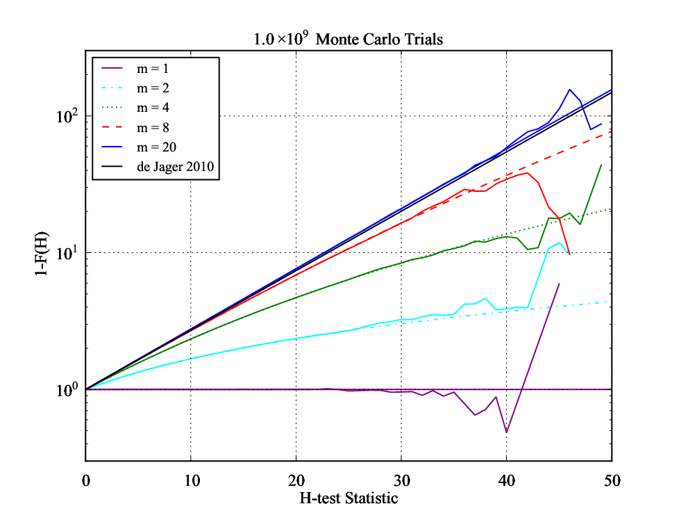
We validated our results with Monte Carlo simulations of the $H_{20}$ statistic in the asymptotic null case. Specifically, for each realization of $H_{20}$ , we drew $20$ realizations from a $\chi^{2}$ distribution with one degree of freedom and determined $H$ accordingly (with $c=4$ .) In Figure 10, we show the results of $10^{9}$ Monte Carlo trials for a variety of maximum harmonics. The results are in good agreement with the asymptotic distribution derived here.

A.4. General Properties for $m\geq 10$

Although the asymptotic calibration for $H_{20}$ has been previously characterized by Monte Carlo [21, 20], the analytic solution extends the calibration to an arbitrary collection of harmonics. (The method used here to develop the asymptotic distribution can be easily extended to cases where the harmonics are not sequential, e.g. a test incorporating only the 2nd, 10th, and 20th harmonics. However, for simplicity’s sake we retain the original formulation of an inclusive set of harmonics.)

It is apparent from Figure 10 that the distributions approach a limiting distribution as $m$ , the maximum harmonic, becomes large. Indeed, as we see in Figure 11, for $m\geq 10$ , there is very little difference in the tail probability for “practical” values of $H$ . For instance, the chance probabilities of observing $H_{m}>50$ for any harmonic $m\geq 10$ are all within a factor of 2 of each other, a negligible distinction at this significance level, and for $H_{m}<50$ , the discrepancy is even smaller. We conclude that, once one has made the decision to choose $m$ large enough to allow for sharply-peaked light curves—and indeed, this is the whole point of the $H$ -test—that there is no penalty for making $m$ as large as feasible. In this sense, the $H$ -test becomes truly omnibus, as $m$ can be chosen large enough to make the test sensitive to light curves with arbitrarily sharp features. Finally, we note a practical formula for the cdf applicable for $m\geq 10$ : $1-F(H)\approx\exp(-0.398405\,H)$ . This is, naturally, quite close to the formula reported by de Jager & Büsching [20]. For $m<10$ , quadratic terms in the exponential are important for an accurate evaluation of the tail probability and the full expression Eq. A10 should be used.