Mass-radius relation of Newtonian self-gravitating Bose-Einstein condensates
with short-range interactions: II. Numerical results

A Newtonian self-gravitating BEC is described by the Gross-Pitaevskii-Poisson system [32, 40]:

$$i\hbar\frac{\partial\psi}{\partial t}=-\frac{\hbar^{2}}{2m}\Delta\psi+m(\Phi+gNm|\psi|^{2})\psi,$$

(1)

$$\Delta\Phi=4\pi GNm|\psi|^{2},$$

(2)

with $g={4\pi a\hbar^{2}}/{m^{3}}$ where $a$ is the s-scattering length (we allow $a$ to be positive or negative) [43]. We write the wave function in the form $\psi({\bf r},t)=A({\bf r},t)e^{iS({\bf r},t)/\hbar}$ where $A$ and $S$ are real, and make the Madelung [36] transformation

$$\rho=Nm|\psi|^{2}=NmA^{2},\qquad{\bf u}=\frac{1}{m}\nabla S,$$

(3)

where $\rho({\bf r},t)$ is the density field and ${\bf u}({\bf r},t)$ the velocity field. The total mass of the configuration is $M=Nm=\int\rho\,d{\bf r}$. We note that the flow is irrotational since $\nabla\times{\bf u}={\bf 0}$. With this transformation, it can be shown that the Gross-Pitaevskii equation (1) is equivalent to the barotropic Euler equations with an additional term called the quantum potential (or quantum pressure). Indeed, one obtains the set of equations

$$\frac{\partial\rho}{\partial t}+\nabla\cdot(\rho{\bf u})=0,$$

(4)

$$\frac{\partial{\bf u}}{\partial t}+({\bf u}\cdot\nabla){\bf u}=-\frac{1}{\rho}\nabla p-\nabla\Phi-\frac{1}{m}\nabla Q,$$

(5)

with

$$Q=-\frac{\hbar^{2}}{2m}\frac{\Delta\sqrt{\rho}}{\sqrt{\rho}},$$

(6)

and

$$p=\frac{2\pi a\hbar^{2}}{m^{3}}\rho^{2}.$$

(7)

The pressure relation (7) corresponds to a polytropic equation of state of the form

$$p=K\rho^{\gamma},\qquad\gamma=1+\frac{1}{n},$$

(8)

with polytropic index $n=1$ (i.e. $\gamma=2$) and polytropic constant $K={2\pi a\hbar^{2}}/{m^{3}}$.

Remark: If dark matter is treated as a collisionless fluid (as in standard models [44, 37]), the evolution of this fluid is fundamentally described by the Vlasov-Poisson system. The hydrodynamic equations without pressure ($\hbar=p=0$) can be obtained if we assume the existence of a single fluid velocity at every spatial position and they cease to be valid after the first time of crossing where multi-streaming generates a range of particles velocities through a given point [45]. In that case, the evolution of the Vlasov-Poisson system becomes very complex and exhibits phenomena of nonlinear Landau damping and phase mixing [46]. The derivation of fluid equations in that context becomes difficult (it amounts to closing the infinite hierarchy of Jeans equations) even if we may argue that a form of local thermodynamical equilibrium and an effective pressure arise as a result of violent relaxation [47]. Alternatively, if dark matter is a self-gravitating BEC, the hydrodynamic equations (4)-(5) are exact for all times since they are rigorously equivalent to the GP equation (1). In that case, the pressure $p$ is due to short-range interactions and non-ideal effects, not to thermal effects [40]. There is also a quantum pressure. These pressure terms prevent multi-streaming and the formation of singularities (caustics), and regularize the dynamics at small scales [48]. Therefore, BEC dark matter behaves like a fluid, contrary to standard CDM that is essentially collisionless.

If we consider a wave function of the form

$$\psi({\bf r},t)=A({\bf r})e^{-i\frac{Et}{\hbar}},$$

(9)

we obtain the time-independent GP equation

$$-\frac{\hbar^{2}}{2m}\Delta\psi+m(\Phi+gNm\psi^{2})\psi=E\psi,$$

(10)

where $\psi({\bf r})\equiv A({\bf r})$ is real and $\rho({\bf r})=Nm\psi^{2}({\bf r})$. The foregoing equation can be rewritten

$$m\Phi+mg\rho-\frac{\hbar^{2}}{2m}\frac{\Delta\sqrt{\rho}}{\sqrt{\rho}}=E,$$

(11)

or, equivalently,

$$m\Phi+mg\rho+Q=E.$$

(12)

In paper I, we have shown that this equation can be obtained from a variational principle, by minimizing the energy functional $E_{tot}$ at fixed mass $M$. Combined with the Poisson equation (2), we obtain an eigenvalue equation for the wave function $\psi({\bf r})$ where the eigenvalue $E$ is the energy. In the following, we shall be interested in the fundamental eigenmode corresponding to the smallest value of $E$. For this mode, the wave function $\psi(r)$ is spherically symmetric and has no node so that the density profile decreases monotonically with the distance.

The time-independent solution (11) can also be obtained from the Euler equations (4)-(6) since they are equivalent to the GP equation. The steady state of the quantum Euler equation (5) obtained by taking $\partial_{t}=0$ and ${\bf u}={\bf 0}$ satisfies

$$\nabla p+\rho\nabla\Phi-\frac{\hbar^{2}\rho}{2m^{2}}\nabla\left(\frac{\Delta\sqrt{\rho}}{\sqrt{\rho}}\right)={\bf 0}.$$

(13)

This is similar to the condition of hydrostatic equilibrium with an additional quantum potential. It describes the balance between pressure due to short-range interactions (scattering), quantum pressure (Heisenberg principle) and gravity. This equation is equivalent to Eq. (11). Indeed, integrating Eq. (13) using Eq. (7), we obtain Eq. (11) where the eigenenergy $E$ appears as a constant of integration. Combining Eq. (13) with the Poisson equation (2), we obtain the fundamental equation of hydrostatic equilibrium with quantum effects

$$-\nabla\cdot\left(\frac{\nabla p}{\rho}\right)+\frac{\hbar^{2}}{2m^{2}}\Delta\left(\frac{\Delta\sqrt{\rho}}{\sqrt{\rho}}\right)=4\pi G\rho.$$

(14)

For the polytropic equation of state (7), we get

$$-\frac{4\pi a\hbar^{2}}{m^{3}}\Delta\rho+\frac{\hbar^{2}}{2m^{2}}\Delta\left(\frac{\Delta\sqrt{\rho}}{\sqrt{\rho}}\right)=4\pi G\rho.$$

(15)

There are three important limits to consider.

The non-interacting case corresponds to $g=a=0$. This is the situation first studied by Ruffini & Bonazzola [10] and revisited by Membrado et al. [49] with another method. In that case, Eq. (15) reduces to

$$\frac{\hbar^{2}}{2m^{2}}\Delta\left(\frac{\Delta\sqrt{\rho}}{\sqrt{\rho}}\right)=4\pi G\rho.$$

(16)

It describes the balance between attractive gravity and repulsive quantum pressure (Heisenberg principle). This equation must be solved numerically. It is found [10, 49] that the density profile decays smoothly to infinity and that the radius containing $99\%$ of the mass is given by $R_{99}=9.9\hbar^{2}/GMm^{2}$.

For $a>0$, we can make the Thomas-Fermi approximation which amounts to neglecting the quantum potential. This is the limit considered by Böhmer & Harko [32]. In that case, Eq. (15) becomes

$$\Delta\rho+\frac{Gm^{3}}{a\hbar^{2}}\rho=0.$$

(17)

It describes the balance between attractive gravity and repulsive short-range interactions (scattering). This equation is equivalent to the Lane-Emden equation for a polytrope of index $n=1$ [6]. It has the analytical solution $\rho(r)=(\rho_{0}R/\pi r)\sin\left(\pi r/{R}\right)$ where $R=\pi(a\hbar^{2}/Gm^{3})^{1/2}$ is the radius of the configuration (independent on the mass $M$) and $\rho_{0}=\pi M/4R^{3}$ is the central density.

For $a<0$, the TF approximation leads to collapse since it only keeps the effects of attractive gravity and attractive short-range interactions (scattering). If we want to obtain equilibrium states (for $M<M_{max}$ [40]), we have to solve the complete Eq. (15) expressing the balance between repulsive quantum pressure (Heisenberg principle) and attractive short-range interactions (scattering) and gravity. We could also consider the non-gravitational limit. In that case, Eq. (15) reduces to

$$\frac{4\pi|a|\hbar^{2}}{m^{3}}\Delta\rho+\frac{\hbar^{2}}{2m^{2}}\Delta\left(\frac{\Delta\sqrt{\rho}}{\sqrt{\rho}}\right)=0.$$

(18)

It describes the balance between repulsive quantum pressure (Heisenberg principle) and attractive short-range interactions (scattering). However, in Paper I, we have shown that such equilibria are unstable.

The structure of a self-gravitating BEC with short-range interactions is determined by the condition of hydrostatic equilibrium (15). In the general case, this equation has to be solved numerically. To that purpose, it is convenient to introduce dimensionless variables [49]. We introduce the lengthscale

$$b=\frac{\hbar^{2}}{2GMm^{2}},$$

(19)

which basically corresponds to the radius of a self-gravitating BEC in the absence of short-range interaction [10]. We then define the dimensionless position ${\bf x}$ and the dimensionless density profile $n({\bf x})$ by

$${\bf x}=\frac{{\bf r}}{b},\qquad n({\bf x})=\frac{4\pi b^{3}}{Nm}\rho({\bf r}).$$

(20)

We also introduce the dimensionless eigenenergy $\epsilon$ and the dimensionless gravitational potential $\phi({\bf x})$ through the relations

$\displaystyle\epsilon=\frac{2mb^{2}}{\hbar^{2}}E,\qquad\phi({\bf x})=\frac{2m^{2}b^{2}}{\hbar^{2}}\Phi({\bf r}).$

(21)

Finally, we introduce the dimensionless parameter

$$\chi=\frac{2Na}{b}=\frac{4GM^{2}ma}{\hbar^{2}}.$$

(22)

It is equal to the ratio between $N$ times the scattering length $a$ and the typical radius $b$ of a self-gravitating BEC without interaction. The non-interacting limit corresponds to $\chi\ll 1$ and the TF limit corresponds to $\chi\gg 1$ [40].

In terms of these dimensionless variables, the equation of hydrostatic equilibrium (15) can be rewritten

$$\Delta\left(\frac{\Delta\sqrt{n}}{\sqrt{n}}\right)-\chi\Delta n=n.$$

(23)

The density must satisfy the normalization condition

$\displaystyle\int n({\bf x})\,d{\bf x}=4\pi.$

(24)

Finally, the normalized eigenenergy $\epsilon$ can be obtained from the steady state equation (11) leading to

$\displaystyle\phi+\chi n-\frac{\Delta\sqrt{n}}{\sqrt{n}}=\epsilon,$

(25)

where $n({\bf x})$ is the solution of Eq. (23) and $\phi({\bf x})$ is given by

$\displaystyle\phi({\bf x})=-\frac{1}{4\pi}\int\frac{n({\bf x}^{\prime})}{|{\bf x}-{\bf x}^{\prime}|}\,d{\bf x}^{\prime},$

(26)

equivalent to the Poisson equation (2). For a spherically symmetric distribution, Eq. (23) reduces to the ordinary differential equation

	$\displaystyle n^{\prime\prime\prime\prime}+\frac{4}{x}n^{\prime\prime\prime}-\frac{10n^{\prime}n^{\prime\prime}}{nx}+\frac{6n^{\prime 3}}{n^{2}x}-\frac{3n^{\prime\prime\prime}n^{\prime}}{n}-\frac{2n^{\prime\prime 2}}{n}$
	$\displaystyle+\frac{7n^{\prime 2}n^{\prime\prime}}{n^{2}}-\frac{3n^{\prime 4}}{n^{3}}-2n\chi\left(n^{\prime\prime}+\frac{2n^{\prime}}{x}\right)=2n^{2},$		(27)

where the prime ^′ denotes $d/dx$. The normalization condition (24) takes the form

$\displaystyle\int_{0}^{+\infty}nx^{2}\,dx=1,$

(28)

and the steady state equation (25) becomes

$\displaystyle\epsilon=\phi+\chi n-\frac{n^{\prime\prime}}{2n}-\frac{n^{\prime}}{nx}+\frac{n^{\prime 2}}{4n^{2}}.$

(29)

The density behaves near the origin like $n(x)\simeq n_{0}+n_{2}x^{2}+...$. Taking the limit $x\rightarrow 0$ in Eq. (29), and using the field equation (26), we find that

$\displaystyle\epsilon=-\int_{0}^{+\infty}n(x)x\,dx+\chi n_{0}-\frac{3n_{2}}{n_{0}}.$

(30)

The procedure to determine the equilibrium state is now clear. We first have to solve the differential equation (27) with the boundary conditions $n(0)=n_{0}$, $n^{\prime}(0)=n^{\prime\prime\prime}(0)=0$ and $n^{\prime\prime}(0)=2n_{2}$. The constants $n_{0}$ and $n_{2}$ have to be determined so as to yield a physical density profile at infinity and satisfy the normalization condition (28). Finally, the eigenenergy $\epsilon$ is given by Eq. (30).

To solve this problem, it is convenient to introduce the function $f(x)=n(x)/n_{0}$ and make the change of variables $X=n_{0}^{1/4}x$ and $\mu=n_{0}^{1/2}\chi$. We thus have to solve the ordinary differential equation

	$\displaystyle f^{\prime\prime\prime\prime}+\frac{4}{X}f^{\prime\prime\prime}-\frac{10f^{\prime}f^{\prime\prime}}{fX}+\frac{6f^{\prime 3}}{f^{2}X}-\frac{3f^{\prime\prime\prime}f^{\prime}}{f}-\frac{2f^{\prime\prime 2}}{f}$
	$\displaystyle+\frac{7f^{\prime 2}f^{\prime\prime}}{f^{2}}-\frac{3f^{\prime 4}}{f^{3}}-2f\mu\left(f^{\prime\prime}+\frac{2f^{\prime}}{X}\right)=2f^{2},$		(31)

with the boundary conditions

$\displaystyle f(0)=1,\quad f^{\prime}(0)=f^{\prime\prime\prime}(0)=0,\quad f^{\prime\prime}(0)=\frac{2n_{2}}{n_{0}^{3/2}}\equiv A_{2}.$

For given $\mu$, the constant $A_{2}$ is determined so as to yield a physical density profile at infinity (see below). Then, the constant $n_{0}$ is determined by the normalization condition (28) which becomes

$\displaystyle\frac{1}{n_{0}^{1/4}}=\int_{0}^{+\infty}f(X)X^{2}\,dX.$

(33)

Once $A_{2}$ and $n_{0}$ are known, we can obtain the coefficient $n_{2}=A_{2}n_{0}^{3/2}/2$, the parameter $\chi=\mu/n_{0}^{1/2}$ and the normalized eigenenergy

$\displaystyle\epsilon=-\sqrt{n_{0}}\int_{0}^{+\infty}f(X)X\,dX+\sqrt{n_{0}}\mu-\frac{3n_{2}}{n_{0}}.$

(34)

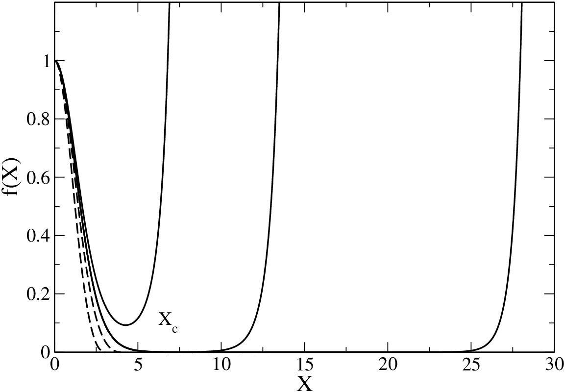
The numerical procedure that was followed to determine the proper value of $A_{2}$, denoted $(A_{2})_{*}$, can be understood from the example shown in Fig. 1. If we solve the differential equation (31) with $A_{2}>(A_{2})_{*}$ (full lines), the density profile reaches a minimum $f_{min}$ at $X=X_{c}$ before increasing indefinitely. As $A_{2}$ approaches $(A_{2})_{*}$ from above, the point $X_{c}$ is pushed further and further away while $f_{min}$ decreases. Therefore, the divergence of the density occurs at larger and larger radii. On the other hand, if we solve the differential equation with $A_{2}<(A_{2})_{*}$ (dashed lines), the density profile decreases until a point $X=X_{c}$ at which the program breaks down because the density achieves too small values ($<10^{-11}$). As $A_{2}$ approaches $(A_{2})_{*}$ from below, the point $X_{c}$ is pushed further and further away so that the “break down” occurs at larger and larger radii. Ideally, if we could start exactly from $(A_{2})_{*}$, the point $X_{c}$ would be rejected to $+\infty$ and the density profile would gently decrease towards zero at infinity. In practice, it is impossible to obtain the “exact” value of $(A_{2})_{*}$. Furthermore, it is shown in Fig. 2 that the value of $X_{c}$ increases very slowly (logarithmically) with the distance $|A_{2}-(A_{2})_{*}|$ to the exact value, so that a huge precision on the value of $A_{2}$ is needed to obtain large values of $X_{c}$. Let us call $X_{max}$ the largest value of $X_{c}$ that we have been able to obtain numerically. For $\chi=\mu=0$, we have determined $(A_{2})_{*}$ with a precision of the order of $10^{-12}$, i.e. $(A_{2})_{*}\simeq-0.612386937160$, to get $X_{max}\simeq 18.66$. The normalized central density and the normalized eigenenergy are found to be $n_{0}\simeq 6.911\,10^{-3}$ and $\epsilon\simeq-8.138\,10^{-2}$. Finally, the radius $x$ containing $99\%$ of the mass is $\Lambda_{99}\simeq 19.89$. These values are consistent with those obtained in [49].

More generally, we have solved this shooting problem for several values of $\mu$. The series of equilibria, that will be studied in the following sections, is parameterized by $\mu$ taking values between $-\infty$ and $+\infty$. Figure 3 shows that the parameter $\chi$ is not a monotonic function of $\mu$ in the region corresponding to negative scattering lengths ($a<0$). Indeed, $\chi$ starts from $0^{-}$ when $\mu\rightarrow-\infty$, reaches a minimum value $\chi_{*}\simeq-4.100$ at $\mu_{*}\simeq-1.000$, returns to $0$ at $\mu=0$ and finally increases to $+\infty$ when $\mu\rightarrow+\infty$. The TF limit corresponds to $\mu\rightarrow+\infty$, the non-interacting limit corresponds to $\mu=0$ and the non-gravitational limit corresponds to $\mu\rightarrow-\infty$. The non-monotonicity of $\chi(\mu)$ is associated with an instability. This is related to the Poincaré theorem (see, e.g., [50, 51]) since the parameter $\chi$ plays the role of the mass for a given scattering length $a$. Since the stable equilibrium configurations are minima of energy at fixed mass [40], a direct application of the Poincaré theorem (see Sec. IV.4) implies that a change of stability occurs at a turning point of mass, hence of $\chi$. Since we know that the system is stable in the TF limit (because it is equivalent to a polytrope of index $\gamma=2$ larger than the critical index $\gamma_{c}=4/3$ [52]), we conclude from the Poincaré theorem that all the configurations with $\mu>\mu_{*}$ are dynamically stable (S) while all the configurations with $\mu<\mu_{*}$ are unstable (U). In particular, the system is unstable in the non-gravitational limit. The same conclusions have been reached in Paper I based on the analytical model.

As we have seen, the structure of the problem depends on a single control parameter $\chi$ given by Eq. (22). There are, however, two ways to present the results. In the first case, we assume that the scattering length $a$ is fixed and we study how the physical parameters like the radius, the energy, the density,… depend on the mass. This is certainly the most relevant representation for astrophysical problems. In particular, we shall determine the mass-radius relation $M(R)$ of boson stars as was done in the past for white dwarfs [6] and neutron stars [53]. In the second case, we assume that the mass $M$ is fixed and we study how the physical parameters depend on the scattering length. In particular, we shall determine the radius versus scattering length relation $R(a)$. This representation can also be of interest. Therefore, we shall treat the two situations successively. In each case, the physical parameters (mass, radius, scattering length,…) must be properly normalized as explained below.

$\bullet$ Let us first consider the case where the mass $M$ is fixed. Using the definitions of Paper I, we normalize the scattering length by $a_{Q}=\hbar^{2}/GM^{2}m$, the radius by $R_{Q}=\hbar^{2}/GMm^{2}$, the density by $\rho_{Q}=M/R_{Q}^{3}=G^{3}M^{4}m^{6}/\hbar^{6}$, the total energy by $E_{Q}=GM^{2}/R_{Q}=G^{2}M^{3}m^{2}/\hbar^{2}$ and the eigenenergy by $E_{Q}^{\prime}=GMm/R_{Q}=G^{2}M^{2}m^{3}/\hbar^{2}$. In terms of these variables, we obtain $a/a_{Q}=\chi/4$, $r/R_{Q}=x/2$, $R_{99}/R_{Q}=\Lambda_{99}/2$, $E/E_{Q}^{\prime}=2\epsilon$ and $\rho(r)/\rho_{Q}=(2/\pi)n(x)$. The TF limit is valid for $a\gg a_{Q}$ and the non-interacting limit for $a\ll a_{Q}$.

$\bullet$ Let us now consider the case where the scattering length $a$ is fixed. We normalize the mass by $M_{a}=\hbar/\sqrt{Gm|a|}$, the radius by $R_{a}=(|a|\hbar^{2}/Gm^{3})^{1/2}$, the density by $\rho_{a}=M_{a}/R_{a}^{3}=Gm^{4}/a^{2}\hbar^{2}$, the total energy by $E_{a}=GM_{a}^{2}/R_{a}=\hbar(Gm)^{1/2}/|a|^{3/2}$ and the eigenenergy by $E_{a}^{\prime}=GM_{a}m/R_{a}=Gm^{2}/|a|$. In terms of these variables, we have $M/M_{a}=\sqrt{|\chi|}/2$, $r/R_{a}=x/\sqrt{|\chi|}$, $R_{99}/R_{a}=\Lambda_{99}/\sqrt{|\chi|}$, $E/E_{a}^{\prime}=\epsilon|\chi|/2$ and $\rho(r)/\rho_{a}=\chi^{2}n(x)/8\pi$. The TF limit is valid for $M\gg M_{a}$ and the non-interacting limit for $M\ll M_{a}$.

We can now plot the fundamental curves in the two situations described above. The procedure is the following. For a given value of $\mu$, we determine successively $(A_{2})_{*}$, $n_{0}$, $n_{2}$, $\chi$ and $\epsilon$. Then, we obtain the density profile $n(x)$. From the density profile $n(x)$, we obtain the value $\Lambda_{99}$ of the radius $x$ containing $99\%$ of the mass. Finally, by varying $\mu$ between $-\infty$ and $+\infty$, we obtain the fundamental curves (parametrized by $\mu$) for a fixed value of the scattering length or for a fixed value of the total mass by using the parameters defined above. The quantities that appear in these curves (mass, radius, density, energy,…) are dimensionless so that we are not required to specify the characteristics of the bosons (that are necessarily uncertain). In this sense, our approach is very general and can model different systems such as (mini) boson stars and galactic halos. In Appendix A, we make numerical applications in order to compare our results with real astrophysical objects.

The mass-radius relation for a fixed value of the scattering length is plotted in Figs. 4, 5, 6 and 7 for positive and negative scattering lengths ($R_{99}$ corresponds to the radius containing $99\%$ of the mass). In the non-interacting case $a=0$, or for $M\rightarrow 0$ when $a\neq 0$, we find

$$R_{99}=9.946\frac{\hbar^{2}}{GMm^{2}},$$

(35)

in agreement with previous works [10, 49]. In the TF limit valid for $M\rightarrow+\infty$ (when $a>0$) [32], we have the analytical result

$$R_{99}\sim 2.998\left(\frac{a\hbar^{2}}{Gm^{3}}\right)^{1/2}.$$

(36)

For $a>0$, there exists an equilibrium state for all the values of the mass $M$ and the configurations are stable (S), see Figs. 4 and 5. The radius (36) represents the minimum radius achievable by the system [40]. For $a<0$, there exists a maximum mass

$\displaystyle M_{max}=1.012\frac{\hbar}{\sqrt{|a|Gm}},$

(37)

corresponding to the radius

$\displaystyle R^{*}_{99}=5.5\left(\frac{|a|\hbar^{2}}{Gm^{3}}\right)^{1/2}.$

(38)

There is no equilibrium state with $M>M_{max}$, see Figs. 6 and 7. In that case, the system is expected to collapse and form a black hole ⁴⁴ 4 The maximum mass (37) that we obtain in the case of negative scattering lengths (attractive short-range interactions) is a purely Newtonian result. In this sense, it is very different from the maximum mass of white dwarf stars [6] and boson stars [9, 10, 17] whose existence is due to relativistic effects. Attractive short-range interactions add to the gravitational attraction and make the system very unstable. This is why there exists a maximum mass even in the Newtonian theory. Of course, if we want to describe the collapse of the system for $M>M_{max}$ and the formation of a black hole, we must ultimately resort to general relativity.. For $M<M_{max}$, the right branch ($R>R_{*}$) is stable (S) and the left branch ($R<R_{*}$) is unstable (U). As indicated previously, the change of stability occurs at the turning point of mass in agreement with the Poincaré theorem (see Paper I and Sec. IV.4).

The mass-radius relation $M(R)$ for a fixed value of the scattering length $a$ has been studied in Paper I by using a Gaussian ansatz. This leads to the approximate analytical relation

$\displaystyle M=\frac{2\sigma}{\nu}\frac{\frac{\hbar^{2}}{Gm^{2}R}}{1-\frac{6\pi\zeta a\hbar^{2}}{\nu Gm^{3}R^{2}}},$

(39)

with $\sigma=3/4$, $\zeta=1/(2\pi)^{3/2}$, $\nu=1/\sqrt{2\pi}$. We can also express the radius as a function of the mass as

$\displaystyle R=\frac{\sigma}{\nu}\frac{\hbar^{2}}{GMm^{2}}\left(1\pm\sqrt{1+\frac{6\pi\zeta\nu}{\sigma^{2}}\frac{GmM^{2}a}{\hbar^{2}}}\right),$

(40)

with $+$ when $a\geq 0$ and $\pm$ when $a<0$. This relation is compared with the exact mass-radius relation in Figs. 4 and 6 for positive and negative scattering lengths. The analytical model gives the same scalings as Eqs. (35), (36), (37) and (38) with the prefactors $8.955$, $4.125$, $1.085$ and $4.125$ respectively. We see that the agreement between the analytical relation and the numerical one is qualitatively correct in all cases. It is also quantitatively good, except in the TF limit. This is because, in the TF limit, the density has a compact support that is poorly represented by a Gaussian distribution.

The eigenenergy $E$ is plotted as a function of the mass $M$ in Figs. 8 and 9 for positive and negative scattering lengths. In the non-interacting case $a=0$, or for $M\rightarrow 0$ when $a\neq 0$, we obtain

$\displaystyle E=-0.1628\frac{G^{2}M^{2}m^{3}}{\hbar^{2}}.$

(41)

In the TF limit valid for $M\rightarrow+\infty$ (when $a>0$), we have the analytical result [40]:

$\displaystyle E=-\frac{1}{\pi}\frac{G^{3/2}m^{5/2}M}{a^{1/2}\hbar}.$

(42)

For $a<0$, the eigenenergy corresponding to the point of maximum mass is

$\displaystyle E_{*}=-0.36\frac{Gm^{2}}{|a|}.$

(43)

The eigenenergy $E$ can be estimated analytically from the Gaussian ansatz by using the results of Paper I (see in particular Sec. III.B). Using Eqs. (I-77) and (I-83), we get

$\displaystyle E=\sigma\frac{\hbar^{2}}{mR^{2}}+2{\zeta}\frac{2\pi a\hbar^{2}M}{m^{2}R^{3}}-2\nu\frac{GMm}{R},$

(44)

where the mass and the radius are related to each other by Eq. (39). We can therefore express $E$ as a function of $R$ alone

$$E=-\sigma\frac{\hbar^{2}}{mR^{2}}\left(4\frac{1-\frac{2\pi\zeta a\hbar^{2}}{\nu Gm^{3}R^{2}}}{1-\frac{6\pi\zeta a\hbar^{2}}{\nu Gm^{3}R^{2}}}-1\right).$$

(45)

Then, eliminating the radius between $M(R)$ and $E(R)$, we obtain $E$ as a function of $M$ in parametric form. Alternatively, we can substitute the analytical expression of $R(M)$ given by Eq. (40) in Eq. (44). In the non-interacting case, using $E=3W/2N$ [40] and Eqs. (I-83) and (I-93), we obtain

$\displaystyle E=-\frac{3\nu^{2}}{4\sigma}\frac{G^{2}M^{2}m^{3}}{\hbar^{2}}.$

(46)

In the TF approximation (for $a>0$), using $E=4W/3N$ [40] and Eqs. (I-83) and (I-94), we find that

$\displaystyle E=-\frac{4\nu^{3/2}}{3(6\pi\zeta)^{1/2}}\frac{G^{3/2}m^{5/2}M}{a^{1/2}\hbar}.$

(47)

In the non-gravitational limit (for $a<0$), using $E=-\Theta_{Q}/3N$ [40] and Eqs. (I-83) and (I-96), we get

$\displaystyle E=-\frac{\sigma^{3}}{3(3\pi\zeta)^{2}}\frac{\hbar^{2}m}{M^{2}a^{2}}.$

(48)

Finally, combining Eqs. (44), (I-99) and (I-100), the eigenenergy corresponding to the point of maximum mass is found to be

$\displaystyle E_{*}=-\frac{5\sigma\nu}{18\pi\zeta}\frac{Gm^{2}}{|a|}.$

(49)

This returns the scalings of Eqs. (41), (42) and (43) with the prefactors $-0.1592$, $-0.3071$ and $-0.4166$ (in the non-gravitational case, the prefactor is $-0.3927$). We see in Figs. 8 and 9 that the agreement with the numerical curves is fairly good, even in the TF limit. This is because the value of the energy is less sensitive to the detailed form of the density profile. Close to the maximum mass (for $a<0$), the agreement is good but not excellent.

We can also estimate the total energy from the Gaussian ansatz by using the results of Paper I (see in particular Sec. III.B). Using Eqs. (I-75) and (I-83), we get

$\displaystyle E_{tot}=\sigma\frac{\hbar^{2}M}{m^{2}R^{2}}+{\zeta}\frac{2\pi a\hbar^{2}M^{2}}{m^{3}R^{3}}-\nu\frac{GM^{2}}{R},$

(50)

where the mass and the radius are related to each other by Eq. (39). We can therefore express $E_{tot}$ as a function of $R$ alone

$$E_{tot}=-\frac{2\sigma^{2}}{\nu}\left(2\frac{1-\frac{2\pi\zeta a\hbar^{2}}{\nu Gm^{3}R^{2}}}{1-\frac{6\pi\zeta a\hbar^{2}}{\nu Gm^{3}R^{2}}}-1\right)\frac{\frac{\hbar^{4}}{Gm^{4}R^{3}}}{1-\frac{6\pi\zeta a\hbar^{2}}{\nu Gm^{3}R^{2}}}.$$

(51)

Then, eliminating the radius between $M(R)$ and $E_{tot}(R)$, we obtain $E_{tot}$ as a function of $M$ in parametric form. Alternatively, we can substitute the analytical expression of $R(M)$ given by Eq. (40) in Eq. (50). In the non-interacting case, using $E_{tot}=NE/3$ [40], we obtain

$\displaystyle E_{tot}=-\frac{\nu^{2}}{4\sigma}\frac{G^{2}M^{3}m^{2}}{\hbar^{2}}.$

(52)

In the TF approximation (for $a>0$), using $E_{tot}=NE/2$ [40], we find that

$\displaystyle E_{tot}=-\frac{2\nu^{3/2}}{3(6\pi\zeta)^{1/2}}\frac{G^{3/2}m^{3/2}M^{2}}{a^{1/2}\hbar}.$

(53)

In the non-gravitational limit (for $a<0$), using $E_{tot}=-NE$ [40], we get

$\displaystyle E_{tot}=\frac{\sigma^{3}}{3(3\pi\zeta)^{2}}\frac{\hbar^{2}}{Ma^{2}}.$

(54)

Finally, combining Eqs. (50), (I-99) and (I-100), the total energy corresponding to the point of maximum mass is found to be

$\displaystyle E_{tot}^{*}=-\frac{\sigma^{2}\nu^{1/2}}{3(6\pi\zeta)^{3/2}}\frac{\hbar(Gm)^{1/2}}{|a|^{3/2}}.$

(55)

The prefactors are $-0.05307$, $-0.1536$, $0.3927$ and $-0.09045$ respectively. The total energy $E_{tot}$ obtained with the Gaussian ansatz is plotted as a function of the mass $M$ in Figs. 10 and 11 for positive and negative scattering lengths.

The central density $\rho_{0}$ vs mass $M$ is plotted in Figs. 12 and 13 for positive and negative scattering lengths. In the non-interacting case $a=0$, or for $M\rightarrow 0$ when $a\neq 0$, we find that

$${\rho}_{0}=4.400\,10^{-3}\frac{G^{3}M^{4}m^{6}}{\hbar^{6}}.$$

(56)

In the TF limit valid for $M\rightarrow+\infty$ (when $a>0$) [32], we have the analytical result

$${\rho}_{0}=\frac{1}{4\pi^{2}}\frac{G^{3/2}Mm^{9/2}}{a^{3/2}\hbar^{3}}.$$

(57)

When $a<0$, the central density at the point of maximum mass is

$$({\rho}_{0})_{*}=0.04\frac{Gm^{4}}{a^{2}\hbar^{2}}.$$

(58)

It is interesting to compare these results with those obtained from the Gaussian ansatz. In that case, the central density is related to the mass and to the radius by

$\displaystyle\rho_{0}=\frac{M}{\pi^{3/2}R^{3}}.$

(59)

Combining this relation with Eq. (39), we obtain the central density as a function of the radius

$\displaystyle\rho_{0}=\frac{2\sigma}{\nu\pi^{3/2}}\frac{\frac{\hbar^{2}}{Gm^{2}R^{4}}}{1-\frac{6\pi\zeta a\hbar^{2}}{\nu Gm^{3}R^{2}}}.$

(60)

Eliminating the radius between $M(R)$ and $\rho_{0}(R)$, we obtain the approximate central density versus mass relation in parametric form. Alternatively, we can substitute the analytical expression of $R(M)$ given by Eq. (40) in Eq. (59). In the non-interacting case, we obtain

$${\rho}_{0}=\frac{\nu^{3}}{8\sigma^{3}\pi^{3/2}}\frac{G^{3}M^{4}m^{6}}{\hbar^{6}}.$$

(61)

In the Thomas-Fermi limit (when $a>0$), we find that

$${\rho}_{0}=\left(\frac{\nu}{6\pi^{2}\zeta}\right)^{3/2}\frac{G^{3/2}Mm^{9/2}}{a^{3/2}\hbar^{3}}.$$

(62)

In the non-gravitational limit (when $a<0$), we get

$${\rho}_{0}=\left(\frac{\sigma}{3\pi^{3/2}\zeta}\right)^{3}\frac{m^{3}}{M^{2}|a|^{3}}.$$

(63)

Finally, the central density at the point of maximum mass is found to be

$$({\rho}_{0})_{*}=\frac{\sigma\nu}{\pi^{3/2}(6\pi\zeta)^{2}}\frac{Gm^{4}}{a^{2}\hbar^{2}}.$$

(64)

This returns the scalings of Eqs. (56), (57) and (58) with the prefactors $0.003378$, $0.03456$ and $0.03751$ (the prefactor in the non-gravitational limit is $0.3535$). The analytical mass-central density relation is compared with the exact relation in Figs. 12 and 13. The agreement is fairly good, except in the TF limit (when $a>0$). Close to the maximum mass (when $a<0$), the agreement is good but not perfect. Some density profiles $\rho(r)$ are represented in Figs. 14, 15, 16 for positive and negative scattering lengths and different values of $M$.

It is interesting to develop an analogy with thermodynamics. We have seen in Paper I that stable steady states of the GPP system, or equivalently of the quantum barotropic Euler-Poisson system, correspond to (local) minima of the energy functional (see Eqs. (I-56)-(I-64)):

	$\displaystyle E_{tot}[\rho,{\bf u}]=\int\rho\frac{{\bf u}^{2}}{2}\,d{\bf r}+\frac{\hbar^{2}}{2m^{2}}\int(\nabla\sqrt{\rho})^{2}\,d{\bf r}$
	$\displaystyle+\frac{2\pi a\hbar^{2}}{m^{3}}\int\rho^{2}\,d{\bf r}+\frac{1}{2}\int\rho\Phi\,d{\bf r}.$		(65)

at fixed mass $M$. We thus have to study the variational problem

$\displaystyle\min_{\rho,{\bf u}}\{E_{tot}[\rho,{\bf u}]\,|\,M[\rho]=M\}.$

(66)

The critical points, cancelling the first order variations of constrained total energy, are given by $\delta E_{tot}-\alpha\delta M=0$ where $\alpha$ is a Lagrange multiplier associated with the conservation of mass that can be interpreted as a chemical potential. These first order variations lead to the steady state equation (11) provided that we make the identification $\alpha=E/m$. This shows that the eigenenergy $E$ can be interpreted as a chemical potential. As a result, Figs. 8 and 9 give the chemical potential $\alpha=\partial E_{tot}/\partial M$ (conjugate quantity) as a function of the mass $M$ (conserved quantity). Similarly, in thermodynamics, the statistical equilibrium state of a system is obtained by maximizing the entropy $S$ at fixed energy $E$ (see, e.g. [51]). The first order variations are given by $\delta S-\beta\delta E=0$ where $\beta$ is a Lagrange multiplier associated with the conservation of energy that represents the inverse temperature. The caloric curve $\beta(E)$ gives the inverse temperature $\beta=\partial S/\partial E$ (conjugate quantity) as a function of energy $E$ (conserved quantity). Now, using the Poincaré theory of linear series of equilibria, we know that when we plot the conjugate quantity as a function of the conserved quantity, a change of stability can only occur at a turning point of the conserved quantity or at a bifurcation point. In the present case, when $a<0$, the change of stability occurs at the turning point of mass (see Fig. 9). Similarly, in the thermodynamics of self-gravitating systems, the change of stability occurs at the turning point of energy in the microcanonical ensemble or at the turning point of temperature (equivalent to the turning point of mass) in the canonical ensemble [51]. Finally, since $\delta E_{tot}=\delta M=0$ at the turning point of mass, we conclude that the curve $E_{tot}(M)$ presents a cusp at that point (see Fig. 11). Similarly, in thermodynamics, since $\delta S=\delta E=0$ at the turning point of energy, the curve $S(E)$ presents a cusp at that point (see Fig. 4 in [54]).

Let us recapitulate: For $a>0$, the series of equilibria containing all the critical points of the variational problem (66) is parametrized by $\mu$ going from $\mu\rightarrow+\infty$ (TF limit) to $\mu\rightarrow 0$ (non-interacting limit). The series of equilibria $R(M)$, $E(M)$ or $E_{tot}(M)$ is monotonic. Since the system is stable in the TF limit (see Sec. III.2), we conclude from the Poincaré theorem that the whole series of equilibria is stable for $a>0$. By continuity, the non-interacting BEC ($\mu=a=0$) is also stable. For $a<0$, the series of equilibria is parametrized by $\mu$ going from $\mu\rightarrow 0$ (non-interacting limit) to $\mu\rightarrow-\infty$ (non-gravitational limit). The series of equilibria $R(M)$, $E(M)$ or $E_{tot}(M)$ is non-monotonic. There is a turning point of mass at $M=M_{max}$ corresponding to $\mu=\mu_{*}\simeq-1.000$. For $M>M_{max}$ there is no solution to the variational problem (66) and for $M<M_{max}$ there are two solutions with the same mass. Since the system is stable in the non-interacting limit $\mu=a=0$ (as we have just seen), we conclude from the Poincaré theorem that the system is stable for $\mu>\mu_{*}$ and unstable for $\mu<\mu_{*}$ (this corresponds to high central densities). This leads to the stability/instability regions shown in Figs 4-13.

The radius vs scattering length relation for a fixed value of the total mass is plotted in Figs. 17 and 18 ($R_{99}$ corresponds to the radius containing $99\%$ of the mass). In the non-interacting case $a=0$, the radius is given by Eq. (35) and in the TF limit $a\rightarrow+\infty$, it is given by Eq. (36). For $a<0$, there exists a minimum scattering length

$\displaystyle a_{min}=-1.025\frac{\hbar^{2}}{GM^{2}m},$

(67)

corresponding to the radius

$\displaystyle R_{99}^{*}=5.6\frac{\hbar^{2}}{GMm^{2}}.$

(68)

There is no equilibrium state when $a<a_{min}$. In that case, the system is expected to collapse and form a black hole. For $a>a_{min}$, the upper line ($R>R_{*}$) is stable (S) and the lower line ($R<R_{*}$) is unstable (U).

References

- [1] A.G. Riess et al., Astron. J. 116, 1009 (1998); S. Perlmutter et al., Astrophys. J. 517, 565 (1999); P. de Bernardis et al., Nature 404, 995 (2000); S. Hanany et al., Astrophys. J. 545, L5 (2000)
- [2] F. Zwicky, Helv. Phys. Acta 6, 110 (1933); see also S. Smith, Astrophys. J. 83, 23 (1936) and F. Zwicky, Astrophys. J. 86, 217 (1937)
- [3] V.C. Rubin, W.K. Ford, N. Thonnard, Astrophys. J. 238, 471 (1980)
- [4] M. Persic, P. Salucci, F. Stel, Mon. Not. R. Astron. Soc. 281, 27 (1996)
- [5] M. Milgrom, Astrophys. J. 270, 365 (1983)
- [6] S. Chandrasekhar, Stellar structure (University of Chicago Press, Chicago, 1939)
- [7] J.R. Primack, D. Seckel, B. Sadoulet, Annu. Rev. Nucl. Part. Sci. 38, 751 (1988)
- [8] J.M. Overduin, P.S. Wesson, Phys. Rep. 402, 267 (2004)
- [9] D.J. Kaup, Phys. Rev. 172, 1331 (1968)
- [10] R. Ruffini, S. Bonazzola, Phys. Rev. 187, 1767 (1969)
- [11] W. Thirring, Phys. Lett. B 127, 27 (1983)
- [12] J.D. Breit, S. Gupta, A. Zaks, Phys. Lett. B 140, 329 (1984)
- [13] E. Takasugi, M. Yoshimura, Z. Phys. C 26, 241 (1984)
- [14] J.J. van der Bij, M. Gleiser, Phys. Lett. B 194, 482 (1987)
- [15] F.E. Schunck, E.W. Mielke, Class. Quantum Grav. 20, R301 (2003)
- [16] E.W. Mielke, F.E. Schunck, Nuc. Phys. B 564, 185 (2000)
- [17] M. Colpi, S.L. Shapiro, I. Wasserman, Phys. Rev. Lett. 57, 2485 (1986)
- [18] M. Bianchi, D. Grasso, R. Ruffini, Astron. Astrophys. 231, 301 (1990)
- [19] M.S. Madsen, A.R. Liddle, Phys. Lett. B 251, 507 (1990)
- [20] M.R. Baldeschi, G.B. Gelmini, R. Ruffini, Phys. Lett. B 122, 221 (1983)
- [21] S.J. Sin, Phys. Rev. D 50, 3650 (1994)
- [22] J. Lee, I. Koh, Phys. Rev. D 53, 2236 (1996)
- [23] F.E. Schunck, [astro-ph/9802258]
- [24] F.S. Guzmán, T. Matos, Class. Quantum Grav. 17, L9 (2000)
- [25] W. Hu, R. Barkana, A. Gruzinov, Phys. Rev. Lett. 85, 1158 (2000)
- [26] P.J.E. Peebles, Astrophys. J. 534, L127 (2000)
- [27] J. Goodman, New Astronomy 5, 103 (2000)
- [28] A. Arbey, J. Lesgourgues, P. Salati, Phys. Rev. D 64, 123528 (2001)
- [29] M. Alcubierre, F.S. Guzmán, T. Matos, D. Núñez, L.A. Ureña-López, P. Wiederhold, Class. Quantum. Grav. 19, 5017 (2002)
- [30] M.P. Silverman, R.L. Mallett, Gen. Rel. Grav. 34, 633 (2002)
- [31] A. Arbey, J. Lesgourgues, P. Salati, Phys. Rev. D 68, 023511 (2003)
- [32] C.G. Böhmer, T. Harko, J. Cosmol. Astropart. Phys. 06 (2007) 025
- [33] T. Fukuyama, M. Morikawa, T. Tatekawa, JCAP 06, 033 (2008)
- [34] P. Sikivie, Q. Yang, Phys. Rev. Lett. 103, 111301 (2009)
- [35] J.W. Lee, S. Lim, JCAP 01, 007 (2010)
- [36] E. Madelung, Zeit. F. Phys. 40, 322 (1927)
- [37] P.J.E. Peebles, B. Ratra, Rev. Mod. Phys. 75, 559 (2003)
- [38] A. Burkert, Astrophys. J. 447, L25 (1995); C. Firmani et al., Mon. Not. R. astr. Soc. 321, 713 (2001); W.J.G. De Blok et al., Mon. Not. R. astr. Soc. 340, 657 (2003); G. Gentile et al., Astrophys. J. 634, L145 (2005); G. Battaglia et al., Astrophys. J. 681, L13 (2008); S.H. Oh et al., [arXiv:1011.0899]
- [39] G. Kauffmann, S.D.M. White, B. Guiderdoni, Mon. Not. R. astr. Soc. 264, 201 (1993); A. Klypin, A.V. Kravtsov, O. Valenzuela, Astrophys. J. 522, 82 (1999); M. Kamionkowski, A.R. Liddle, Phys. Rev. Lett. 84, 4525 (2000)
- [40] P.H. Chavanis, [arXiv:1103.2050] (Paper I)
- [41] P.H. Chavanis, in preparation (Paper III)
- [42] P.H. Chavanis, [arXiv:1103.2698]
- [43] F. Dalfovo, S. Giorgini, L.P. Pitaevskii, S. Stringari, Rev. Mod. Phys. 71, 463 (1999)
- [44] Peebles P.J.E., 1980, The Large-Scale Structure of the Universe. Princeton University Press
- [45] M. Vergassola, B. Dubrulle, U. Frisch, A. Noullez, Astron. Astrophys. 289, 325 (1994)
- [46] H. Kandrup, Astrophys. J. 500, 120 (1998)
- [47] P.H. Chavanis, J. Sommeria, R. Robert, Astrophys. J. 471, 385 (1996)
- [48] P.H. Chavanis, [arXiv:1103.3219]
- [49] M. Membrado, A.F. Pacheco, J. Sanudo, Phys. Rev. A 39, 4207 (1989)
- [50] J. Katz, Found. Phys. 33, 223 (2003)
- [51] P.H. Chavanis, Int. J. Mod. Phys. B 20, 3113 (2006)
- [52] J. Binney, S. Tremaine, Galactic Dynamics (Princeton, NJ: Princeton University Press, 1987)
- [53] S.L. Shapiro, S.A. Teukolsky, Black holes, white dwarfs and neutron stars (Wiley, New York, 1983)
- [54] P.H. Chavanis, Phys. Rev. E 65, 056123 (2002)
- [55] P.H. Chavanis, T. Harko, arXiv:1108.3986