Perturbations of SNe Ia lightcurves, colors and spectral features by circumstellar dust
Abstract
It has been suggested that multiple scattering on circumstellar dust could explain the non-standard reddening observed in the line-of-sight to Type Ia supernovae. In this work we use Monte Carlo simulations to examine how the scattered light would affect the shape of optical lightcurves and spectral features. We find that the effects on the lightcurve widths, apparent time evolution of color excess and blending of spectral features originating at different photospheric velocities should allow for tests of the circumstellar dust hypothesis on a case by case basis. Our simulations also show that for circumstellar shells with radii cm, the lightcurve modifications are well described by the empirical parameter and intrinsic color variations of order arise naturally. For large shell radii an excess lightcurve tail is expected in band, as observed in e.g. SN 2006X.
Subject headings
dust, extinction — Interstellar medium, nebulae :distance scale — Cosmology : supernovae: general — Stars : supernovae individual SN 2006X – StarsI. Introduction
A dramatic breakthrough in cosmology took place more than a decade ago when the accelerated expansion of the universe was discovered through Type Ia supernovae (SNe Ia) used as standardizable candles [37, 34]. SNe Ia remain among the best tools to investigate the energy content of the universe, as demonstrated by recent very successful surveys of high- SNe [3, 48, 39, 25, 23, 2]. However, the progress for precision cosmology is hampered by systematic uncertainties, notably a potential drift in the SN Ia luminosity and intrinsic colors with cosmic time and the impact of changing dust extinction properties along the line of sight [30]. The standardization of SNe Ia generally uses two parameters: the measured color, typically rest-frame and often one more optical color, and an empirically defined lightcurve shape parameter, such as stretch, [35, 15, 6], [14], [36, 19] or [38, 22]. In this work we examine how multiple scattering of supernova photons on the surrounding material could affect both the lightcurve shapes and colors.
While the reddening of SNe Ia was originally thought to be entirely due to extinction by interstellar dust, there is an increasing body of evidence showing that the measured color excesses to some SN Ia show a steeper wavelength dependence than what is observed for reddened stars in the Milky Way. Likewise, there is no generally accepted model that explains the lightcurve shape variations observed in SNe Ia and its correlations with peak supernova brightness [36].
Following up the work by [42], [13] (hereafter G08) showed that multiple scattering on circumstellar dust could potentially help explaining the low values of the total-to-selective extinction parameter, , observed in the sight lines of near-by Type Ia SNe [9, 10, 26, 45, 29].
A Monte Carlo ray tracing technique was used in G08 to investigate the reddening effects in the presence of circumstellar dust and an approximate reddening law for optical and near-IR wavelengths was derived. Folatelli et al. [11] compared the parametrized model in G08 with high quality data from the Carnegie Supernova Project and found that it provided particularly good fits for the two most reddened SNe Ia in their sample, SN 2005A and SN 2006X. The success of these comparisons calls for further scrutiny of the model. In this work we investigate the impact of multiple scattering on the shapes of SNe Ia optical lightcurves. We explore how the extra wavelength dependent “random walk” of photons in the presence of scatterers affects the width of broad-band filter lightcurves. In particular, reddened “slow decliners” may be compatible with the scenario in G08.
Furthermore, also the strengths of spectroscopic features as a function of time are likely to be affected, since a varying path-length would lead to a superposition of several SN phases. Throughout the paper we point out how observations could put bounds on the size of a hypothetical circumstellar dust shell.
II. Circumstellar dust in the single degenerate scenario
In the currently favored Type Ia scenario, a white dwarf accretes mass from a companion star until the Chandrasekhar limit is reached, at which point instabilities lead to an explosion. However, the model requires the accreting white dwarf to expel material accumulating on its surface through fast stellar winds, km s-1, to avoid the formation of a common envelope between the white dwarf and the donor star which would prevent the explosion [17, 16, 18]. Condensation of dust grains may take place in the ejected matter, possibly also in collisions with the accreting matter. For dust grain growth in stellar winds, the density as a function of distance to the star surface, , is generically expected to scale as , where, , is the stellar wind velocity and is the mass-loss per unit time, typically of order in SNe Ia models.
III. Circumstellar dust destruction by SN Ia luminosity
So far, we have assumed that the supernova explosion site is surrounded by dust. However, the radiation from the supernova itself will sublimate dust grains as these are heated up to K. Thus, assuming that the entire UV-optical luminosity of the supernova, is absorbed by surrounding dust grains, we can compute the radius, , where dust grains, if present at the explosion time, would be depleted. From the radiation balance condition:
| (1) |
where is the effective absorption efficiency and is the Planck-averaged emissivity at . Waxman & Draine [46] studied a similar situation, but for dust surrounding gamma-ray bursts and found that for K, for a mixture of astronomical silicate and graphite grains with typical sizes of 0.1 m. Sollerman et al. [40] have estimated the peak bolometric luminosity of SN Ia to be ergs/s, where the 56Ni mass (in units of solar masses), , has been measured to be between 0.1 and 1.1 [27]. Inserting this peak luminosity ( eV) into Eq. (1), and assuming that all the radiation is absorbed, we find cm ( pc), which we will use as a rough estimate of the region where evaporation of pre-existing dust would take place as a result of the SN heating. A similar estimate of the region that ought to be depleted of dust was done by Pearce & Mayes [33]. Thus, to create a dust shell that would survive the radiation from the supernova explosion, and using the stellar wind velocities and mass-loss rates from Section II, the wind must start about – years prior to the explosion, i.e. of mass must be expelled for any effect of circumstellar dust to be noticeable. For SN 2005gj, a well-studied example of a supernova with significant interaction with the circumstellar environment, Aldering et al. [1] find evidence for mass-loss about 8 years before the explosion. For significant opacity, , the required dust mass can be estimated from the absorption cross-sections in Weingartner & Draine [47] and Draine [7], cmg. Thus, for a thin dust shell at cm, this corresponds to .
We also note that since , intrinsically brighter explosions are likely to have larger , i.e., thinner circumstellar shells. In the following sections we will see that, depending on the size of the outer shell, multiple scattering could generate relations between brightness and lightcurve shapes and colors qualitatively similar to the observed ranges. We note, however, that interaction with dust in the CS material can only broaden the pristine lightcurve, i.e., it is not possible to produce a faster decline than what results from the original supernova explosion.
IV. Multiple scattering of photons around the supernova
A natural effect of light scattering is that it adds flight time to the photons, thereby affecting the observed lightcurve [31, 32]. Next, we start by generalizing the Goobar [13] model: we consider a scenario where the exploding white dwarf ( cm) is at the center of a homogeneous dust shell with an outer radius, (), and an inner radius , where . Note that this will not change any of the results in G08, where was assumed, but it will affect the distribution of photon flight times, i.e., the subject of this paper.
The technique in G08 is extended to investigate the time domain by calculating the total traveled path length, , for each photon before it crosses a plane, , that is perpendicular to the line of sight between the observer and the source, and is located at the the distance, , from the source which is illustrated in Fig. A1. The details for the calculation of the photon travel times are outlined in Sec. Appendix A. The traveled photon path length, , is given by Eq. Appendix A1.
The traveled photon path length is distributed in the interval , with for photons that do not interact with the dust at all. The shape of the distribution of will depend on the radius, , the thickness of the shell, the scattering and absorption properties of the dust, and the dust density. In this work we will quantify the latter in terms of the observed color excess, , relative to the pristine source color. For the scattering and absorption properties we use models consisting of carbonaceous grains and amorphous silicate grains from Weingartner & Draine [47] and Draine [7].
We begin by exploring the scattering distribution for the two extreme scenarios (a) (i.e., a homogeneous dust sphere as in G08), and (b) , i.e., a very thin dust shell. Clearly, the scenario (a) is already challenged by the conclusions in Section III, nevertheless, it serves as a point of reference. The left panel of Fig. 1 shows the distribution of from Monte Carlo simulations of photons with Å. Most photons travel unscattered, and for the rest, there is a rough exponential fall-off of delay times. The dust density was chosen to cause an observed color excess . Furthermore, we are assuming that the dust grain properties correspond to LMC-type dust, although the time distributions for MW-type dust are very similar.
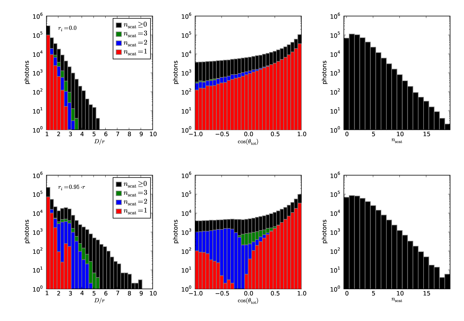
A local minimum can be noted for case (b) around . This can be understood by realizing that photons from the source can only double the path length, , by having a total scattering angle of for this particular setup, which will take it through more dust than for other angles. It is then likely to scatter again, which would result in either a shorter or a longer path. The significance of the minimum will decrease with the density of the dust and the inner radius of the shell .
V. Lightcurve perturbation from multiple scattering
Since the scattering cross-section, scattering angle and albedo are wavelength dependent, the lightcurve perturbations are expected to vary between broad-band filters.
We use the time dependent spectral energy distribution (SED) SN Ia templates from Hsiao et al. [21] (hereafter H07) to build up observed broad-band lightcurves in the presence of circumstellar dust. Thus, we make the simplifying assumption that the empirically derived spectral template is pristine, i.e., not already affected by dust. This is not a major limitation for this analysis, since we are here primarily concerned with relative quantities, such as time-delays or color excess rather than absolute times or fluxes.
Like in G08, we only consider dust grain models from Weingartner & Draine [47] and Draine [7] for Milky-Way dust and LMC dust. In particular, it was found in G08 that LMC dust grains in the circumstellar medium would lead to , while Milky-Way dust lead to . These two grain models approximately bracket the empirically found values for for a large fraction of SNe Ia. In both cases, the extinction law deviated significantly from Galactic extinction [5] in the UV and NIR regions.
For the idealized case considered in this work, a fraction of the photons scatter inside the dust shell and the delay time induced by the multiple scattering will scale with ,
| (2) |
Since the typical rise-time of SNe Ia lightcurves is about 3 weeks, and the fall-time is somewhat longer, we expect significant effects on the shapes of optical lightcurves for cm for increasing optical depth, . On the other hand, for time scales month, i.e., cm, we expect the time perturbations to de-correlate with the lightcurve shape parameters currently used, since these are designed to capture smaller time scale effects.
VI. Lightcurve shape
Existing Type Ia supernova lightcurve fitters [38, 12, 43, 15, 14, 22, 6, 4] use different approaches to take variations of the optical lightcurve shape into account for standardizing SNe Ia. To estimate the effect on the lightcurve shape due to circumstellar dust, we once again consider the two extreme scenarios: (a) and (b) , introduced above.
Fig. 2 shows the time-delay distribution in the band from Monte Carlo simulations as a function of the outer shell radius for cases (a) and (b) where the LMC-type dust density was chosen to cause an observed color excess .

The far left panel of this figure is closely related to the left panel of Fig. 1, except that the dimensionless property has been converted to days by assuming different physical shell radii. First, we note that for very large outer radii, photons that scatter on dust grains have a fairly flat delay probability with respect to the unscattered ones in the first (zero) bin. We also note how the effect that certain photon paths are less likely for a thin shell, as discussed above, propagates to a sharp feature in the delay time distribution.
Also shown in Fig. 2 is how the delayed photons perturb the pristine band lightcurve shape. This reveals how the size of the outer radius, affects (primarily) the post-max shape of the lightcurve. Notably, the largest deviation from the pristine shape can be seen in the tail, more than a month after lightcurve maximum, typically beyond the time range investigated for most reddened supernovae.
VI.1. The fall-time
The most straight-forward method of quantifying post-maximum lightcurve shape is in terms of the magnitude difference between maximum and an arbitrary number of rest-frame days past maximum in a given rest-frame passband. This method of measuring the fall-time was introduced by [36] who chose the rest-frame band and 15 days past maximum respectively, . The simulation results of the evolution of the parameter for a few different CS-scenarios is presented in the far right panel of Fig. 2 and in more detail in Fig. 3.

For cm, decreases with . However, for larger radii, the late photons populate the tail of the lightcurve, i.e., and thus the original pristine lightcurve fall-time at earlier epochs is gradually recuperated, while a plateau is built up at late times. The significance and the variation of the lightcurve tails in the examples shown suggests further studies of the fall-time, also at epochs beyond day . This is illustrated by the right panel of Fig. 3, where two different radii for the same dust configuration can give rise to the same value of , but different values at 35 days past maximum, . For very large radii, both the original values and are recovered. For these extreme radii, the imprint from the CS dust will be found for even later epochs.
Another interesting effect occurs for the dust shell scenario (b) as shown in Fig. 2. The fall-off of the cm curve is initially steeper than the cm curve, but at day past maximum, this changes and the cm curve flattens out and cross the cm curve, while the latter continues to fall. This qualitative behavior can also be seen in real data: two SNe Ia normalized to the same maximum brightness show different relative fall-off for different epochs, as seen in Fig. 4.

VI.2. The rise-time – fall-time relation
The impact of the time-delay effect from scattering on CS material is expected to have a stronger impact on the fall-time than on the rise-time of the lightcurve. The relation between the SNe Ia rise time and has been studied both for high-quality data of well-sampled nearby SNe Ia [41], as well as in a statistical approach for a much larger SDSS-II data set [20]. While Strovink [41] found double-peaked distribution for the relation between rise and fall time, this was not seen by [20]. Fig. 2 reveals that different CS-dust scenarios could give rise to a relation between rise and fall time, even when a single pristine light source is assumed. In Fig. 5 we show this relation for a few different scenarios, together with the results from [41].
The absolute values of any lightcurve parameters determined from our simulations will depend on the corresponding values of the pristine source. Since the lightcurve parameters of the H07 template will roughly reflect the mean values of the SN Ia population, our simulations will only be able to produce lightcurves with longer rise times and smaller than average. In the CS scenario it is reasonable to assume that a “naked” SN Ia template have shorter generic rise time and a faster fall-time, in order to compensate for this we have also applied an add-hoc shift to all curves in Fig. 5 in order to match the data points. Further, assuming that the generic band shape of a “naked” SN Ia is similar to the H07 template that we use here, any modifications to the relative lightcurve properties for different dust scenarios is likely to be of second order, and the general trend and size of the effect should still be valid.

The result from Fig. 5 is that for SNe within a narrow range of observed color excess, CS-dust could naturally give rise to a bi-modal distribution in the relation between rise and fall time for a small sample. However, if the accepted color range is extended, the gap between the two populations will be filled. More generally, it is intriguing that the rise-fall time scatter observed in normal SNe Ia is compatible with our simulations.
VI.3. Time of maximum for different wavelengths
Up to this point we have focused on the effect of circumstellar dust on the rest-frame band, the wavelength range that is traditionally used for doing SN cosmology. Since the scattering and absorption cross-section decreases with wavelength, we expect the delay distribution to affect bluer pass-bands more. One way of studying this is to investigate the impact on the SN rise-time for different filters. However, this is related to comparing the time of maximum in different bands, which is also a property that can be measured quite accurately. Fig. 6 shows the effect on the difference of the time of maximum between the and the bands, , for various CS scenarios. The general trend in the model prediction is that the time between the band and band lightcurve maxima increases for slow decliners. Furthermore, the effect is quite sensitive to optical depth, i.e., to the color excess.

VII. Intrinsic color variations
G08 explicitly describes both how circumstellar dust reddens the pristine source and derives this reddening law. However, as we have seen due to the time delay, mixing of photons originating from different epochs is expected. Since the delay time, , depends on the shell radius, the observed color for a fixed dust amount will have an intrinsic scatter with a magnitude depending on the distribution of the shell size, .
Fig. 7 shows how a few different CS-scenarios could affect both the lightcurve shape and the color at band maximum. As with previous results we can see that the effects of both lightcurve shape and color increases with the amount of CS-dust. There is also degeneracy between different CS scenarios, so no trivial correlation between fall-time and color excess is expected in the CS-scenario. The CS-model thus naturally accommodates an intrinsic color scatter in moderately reddened supernovae, mag, in agreement with observations [29, 24].

VII.1. Time dependent color excess
One of the salient features of the scenario in G08 is that blue photons scatter more than red photons. This implies that blue photons will, on average, be more delayed by multiple scattering since they have a longer path-length before leaving the circumstellar dust environment. This implies that the color excess due to the dust component will acquire time dependence. With respect to a time averaged color excess, the measured color will be redder pre-max turning bluer after max, as shown in Fig. 8. This effect should provide the most stringent bounds on the dust shell sizes allowed by the data. [49] show in their analysis of SN 2006X that once they correct for the color excess around maximum light, the color is about 0.3 mag bluer than the normal unreddened SN 2003du 2 months after lightcurve peak, in qualitative agreement with the CS model prediction.

VIII. Perturbations to the lightcurve shape-brightness relation
Since lightcurve shape is the primary parameter to standardize type Ia supernovae as distance indicators, it is important to investigate how the relation between lightcurve shape and brightness may be affected by the presence of circumstellar dust. As noted in Section III, an intrinsically brighter explosion will deplete more of the surrounding dust, emphasizing the fainter-redder relation. For shell radii cm, the optical lightcurve shape will broaden the lightcurves potentially influencing the empirically derived brighter-broader relation. Is it possible to obtain a correlation between brightness and lightcure shape from the interaction with the circumstellar environment? Although possible, it invokes a somewhat contrived scenario: For shell sizes cm, if the outwards velocity of the circumstellar material, i.e., the white dwarf wind velocity, correlates with the amount of 56Ni powering the explosion, brighter SNe would have large and become slow decliners. We are not aware of any supernova models that have predictions in this respect.
More generally, if the lightcurve shape is a combination of effects, involving both physics of the progenitor system and the material around the white dwarf, then one would expect a residual dependence of brightness on lightcurve shape, even after the main component has been calibrated out. In particular, we note that the optical lightcurve shape beyond 30 days after band peak, will be noticeably affected for a wide range of shell sizes.
IX. The secondary “bump” in the band lightcurve
The type Ia band lightcurve exhibits a secondary maximum approximately 15-30 days after the band lightcurve maximum which, in turn, typically happens within 2 days from the primary band peak [28]. The time gap between the two band peaks, as well as the relative strength of the secondary peak has been shown to correlate with the band lightcurve shape [28].
The implication of the imposed time-delay from scattering on circumstellar dust on the band peaks is shown in Fig. 9. We note that for a constant shell size we expect the brightness difference (upper row) between the peaks, as well as the significance of the secondary peak, to decrease with an increased amount of dust. The effect comes from the fact that photons from the first peak are shifted to both fill the gap between two peaks and emphasize the second bump, and is therefore also correlated with band fall-time and .
If the shell size is allowed to vary, the usual degeneracy between shell size and the amount of dust is obtained for the observables. Despite this degeneracy, it is interesting to note that for a broad range of dust properties and shell sizes, a relation between the band lightcurve properties and is expected.

X. Spectral features
[11] found that different fitted reddening corrections were obtained for their data set depending on whether the reddest SNe were included in the fit or not. For the full data set they obtained , while they fitted if the high-reddened SNe were excluded. In contrast to this, [2] found that redder SNe in the Union2 sample prefer a higher color correction than bluer SNe and speculate that the color correction may very well be more complex than a simple linear relation.
Further, [44] found a bi-modality in the color-magnitude relation over a broad color range, with the two groups preferring different values of independently of the color. They also observed a correlation between the velocity of Si II() and the fitted value of , concluding that objects with high velocity tend to prefer a lower value of than SNe with low velocity.
One possible explanation for the bi-modality could be that the color of the low- SNe primarily originates from CS dust reddening, while the high- objects are dominated by extinction from interstellar dust.
The time-delay of photons from CS dust scattering is expected to blend the spectral energy distributions between different epochs, i.e. a spectral feature for a given epoch will effectively be a superposition of the feature for all previous epochs. Since time-delay distribution varies with wavelength, the amount of blending will also decrease with wavelength. Furthermore, since the minima of the supernova absorption features trace the velocity of the receding photosphere during the first weeks after the explosion, we expect that delayed photons arriving around maximum light will originate from a region further out in the photosphere, i.e., at higher velocities. However, our simulations indicate that these effects are small (see Fig. 10), typically accounting for velocity variations of a few hundred km s-1, i.e., compatible with the velocity scatter between measurements of normal SNe Ia, but not enough to explain significant outliers like SN 2006X [49].

XI. Summary and conclusions
Dust layers surrounding the progenitor systems of SNe Ia could help explain the observed reddening law. In this work, we have performed Monte Carlo simulations that indicate that the scenario with circumstellar dust would also perturb the supernova optical lightcurves in a manner that resembles empirical findings, e.g., an “intrinsic” color variation of arises naturally in our simulations. Since multiple scattering can only introduce a delay in time, the net effect is a broadening of the lightcurve. While the broadening increases monotonically with the density of dust, the relation with the dust shell size is less straight forward: there is an increase for outer radii about cm, while for even larger radii, the late photons populate the tail instead, and the lightcurve width is closer to the original one. We conclude that well sampled multi-band lightcurves of near-by SNe Ia reaching 2-3 months after lightcurve peak would be critical to probe the existence of dust in the circumstellar environment. Our simulations also suggest that for large optical depths, the lightcurve shape perturbation should be notably different before and after maximum. Furthermore, unlike the case for reddening by interstellar dust, color excess should be epoch dependent: redder earlier on and bluer after maximum.
Appendix Appendix A A spherical dust shell
A simple model of a spherical dust-shell with radius, , and inner radius, , where is illustrated in Figure A1. Also shown in the figure is a photon leaving the sphere (solid line).

The current position of the photon is defined by the vector, , and the next position, , is given by , where is the displacement vector .
Photon traveling inside the shell
The impact parameter, , is the minimum distance to the center of the sphere for any given photon-path, and can be defined as.
Here, is given by
If , the photon will cross the inner radius of the shell and then re-enter the shell. This will in turn extend the mean free path of the photon by the amount , which is the length of the path within .
Path length
For each distance between interactions, is added to the total distance traveled by the photon before leaving the sphere. For a scattered photon leaving the sphere, the last distance, , traveled inside the sphere is given by
where . The distance traveled by a scattered photon should be compared to the distance traveled by a non-interacting photon, which means that the distance, , between the surface of the sphere and the plane (thick, solid line in Figure A1) perpendicular to at distance from the center must be added to the total distance, where is given by
The total distance traveled, , can then be summarized as
| (Appendix A1) |
References
- [1] Aldering, G., et al. 2006, ApJ, 650, 510
- [2] Amanullah, R., et al. 2010, ApJ, 716, 712
- [3] Astier, P., et al. 2006, A&A, 447, 31
- [4] Burns, C. R., et al. 2011, AJ, 141, 19
- [5] Cardelli, J. A., Clayton, G. C., & Mathis, J. S. 1989, ApJ, 345, 245
- [6] Conley, A., et al. 2008, ApJ, 681, 482
- [7] Draine, B. T. 2003, ApJ, 598, 1017
- [8] Dwek, E. 1983, ApJ, 274, 175
- [9] Elias-Rosa, N., et al. 2006, MNRAS, 369, 1880
- [10] Elias-Rosa, N., et al. 2008, MNRAS, 384, 107
- [11] Folatelli, G., et al. 2010, AJ, 139, 120
- [12] Goldhaber, G. e. a. 2001, ApJ, 558, 359
- [13] Goobar, A. 2008, ApJ, 686, L103
- [14] Guy, J., et al. 2007, A&A, 466, 11
- [15] Guy, J. e. a. 2005, A&A, 443, 781
- [16] Hachisu, I., & Kato, M. 1999, ApJ, 517, L47
- [17] Hachisu, I., Kato, M., & Nomoto, K. 1996, ApJ, 470, L97+
- [18] Hachisu, I., Kato, M., Nomoto, K., & Umeda, H. 1999, ApJ, 519, 314
- [19] Hamuy, M., Phillips, M. M., Suntzeff, N. B., Schommer, R. A., Maza, J., Smith, R. C., Lira, P., & Aviles, R. 1996, AJ, 112, 2438
- [20] Hayden, B. T., et al. 2010, ApJ, 712, 350
- [21] Hsiao, E. Y., Conley, A., Howell, D. A., Sullivan, M., Pritchet, C. J., Carlberg, R. G., Nugent, P. E., & Phillips, M. M. 2007, ApJ, 663, 1187
- [22] Jha, S., Riess, A. G., & Kirshner, R. P. 2007, ApJ, 659, 122
- [23] Kessler, R., et al. 2009, ApJS, 185, 32
- [24] Kessler, R., et al. 2010, ApJ, 717, 40
- [25] Kowalski, M., et al. 2008, ApJ, 686, 749
- [26] Krisciunas, K., et al. 2007, AJ, 133, 58
- [27] Leibundgut, B. 2000, A&A Rev., 10, 179
- [28] Nobili, S., et al. 2005, A&A, 437, 789
- [29] Nobili, S., & Goobar, A. 2008, A&A, 487, 19
- [30] Nordin, J., Goobar, A., & Jönsson, J. 2008, J. Cosmology Astropart. Phys, 2, 8
- [31] Patat, F. 2005, MNRAS, 357, 1161
- [32] Patat, F., Benetti, S., Cappellaro, E., & Turatto, M. 2006, MNRAS, 369, 1949
- [33] Pearce, G., & Mayes, A. J. 1986, A&A, 155, 291
- [34] Perlmutter, S., et al. 1999, ApJ, 517, 565
- [35] Perlmutter, S. e. a. 1997, Bulletin of the American Astronomical Society, 29, 1351
- [36] Phillips, M. M. 1993, ApJ, 413, L105
- [37] Riess, A. G., et al. 1998, AJ, 116, 1009
- [38] Riess, A. G., Press, W. H., & Kirshner, R. P. 1996, ApJ, 473, 88
- [39] Riess, A. G., et al. 2007, ApJ, 659, 98
- [40] Sollerman, J., et al. 2004, A&A, 428, 555
- [41] Strovink, M. 2007, ApJ, 671, 1084
- [42] Wang, L. 2005, ApJ, 635, L33
- [43] Wang, L., Goldhaber, G., Aldering, G., & Perlmutter, S. 2003, ApJ, 590, 944
- [44] Wang, X., et al. 2009, ApJ, 699, L139
- [45] Wang, X., et al. 2008, ApJ, 675, 626
- [46] Waxman, E., & Draine, B. T. 2000, ApJ, 537, 796
- [47] Weingartner, J. C., & Draine, B. T. 2001, ApJ, 548, 296
- [48] Wood-Vasey, W. M., et al. 2007, ApJ, 666, 694
- [49] Yamanaka, M., et al. 2009, PASJ, 61, 713