Adsorption of polymers at nanowires
Abstract
Low-energy structures of a hybrid system consisting of a polymer and an attractive nanowire substrate as well as the thermodynamics of the adsorption transition are studied by means of Monte Carlo computer simulations. Depending on structural and energetic properties of the substrate, we find different adsorbed polymer conformations, amongst which are spherical droplets attached to the wire and monolayer tubes surrounding it. We identify adsorption temperatures and the type of the transition between adsorbed and desorbed structures depending on the substrate attraction strength.
Keywords:
polymer , adsorption , nanowire , microcanonical analysis1 Introduction
In a systematic study of low-energy states of polymers adsorbed to a stringlike substrate, we recently found a variety of different conformational phases by just changing two basic substrate properties [1]. Among these structures are spherical droplets attached to the string as well as barrellike monolayer conformations surrounding the string. The latter conformations exhibit similarities to single-walled carbon nanotubes.
Generally, the adsorption of polymers on material surfaces or substrates is a crucial and nontrivial process in nature and nanotechnology. It is also known, for example, that the adsorption process or, in fact, the potential of a polymer to adsorb at a semiconductor surface depends essentially on details like the exact position of single monomers in the primary structure of a heteropolymer [2]. However, specific hybrid systems composed of inorganic matter and polymers potentially facilitate the development of completely new nanotechnological devices like sensors for specific single molecules or devices for ultrafast photonics [3, 4].
Hence, fundamental investigations are inevitable for a better understanding of such systems. Computational studies of coarse-grained systems have proven to be adequate and quite useful for this purpose in recent years, both for predicting and interpreting specific and basic behavior of polymer adsorption [5, 6, 7, 8, 2].
Particularly interesting are systems with a cylindrical substrate, like carbon nanotubes. Many of the special properties of these structures, that make them potential candidates for technological applications, can be controlled, influenced or amplified by coating them with polymeric material [3, 4]. In previous computational works, for example, the wetting of cylindrical fibers with polymers or the helical wrapping of single polymers around nanocylinders were studied [9, 10].
In a recent study, we have revealed a more general picture of the adsorption of polymers at different ultrathin cylindrical substrates [1] by performing generalized-ensemble Monte Carlo simulations [11, 12, 13] for a general coarse-grained model of this hybrid system. Here, after describing technical details (Sects. 2 and 3), we focus on specific conformational transitions at very low temperatures (Sect. 4), and discuss in a thermodynamic analysis the adsorption transition at comparatively high temperatures (Sect. 5).
2 The model
For our adsorption study, we employ a coarse-grained off-lattice model, where the polymer consists of identical monomers which are represented by beads without internal structure. These are connected sequentially by stiff bonds of unity length. In order to facilitate future enhancements and the comparison with previous studies (see, e.g., [8]), we introduce a weak stiffness between the bonds, i.e., the polymer is not strictly flexible. The polymer is placed into a simulation box which also contains an attractive thin string located in its center. Its orientation defines the -axis. The edge lengths of this box in and directions with periodic boundary conditions are chosen to be twice as large as the length of the completely stretched polymer. We note that the polymer is not grafted to the string and may move freely in space.
The total energy of the polymer consists of contributions from the Lennard-Jones interaction between all pairs of nonadjacent monomers, a weak bending stiffness and the monomer–string interaction :
| (1) |
with
| (1a) | ||||
| (1b) | ||||
| (1c) |
where is the geometrical distance between two monomers and , is the angle between the two bonds connected to monomer , and is the distance of the th monomer perpendicular to the string. The parameters are set as follows: , such that . The bending stiffness is chosen to be comparatively weak, [14, 8].
The interaction between the string and the monomers is also based on a simple Lennard-Jones potential, where the wire is assumed to have a homogeneous “charge” distribution [9, 10, 8]. The string potential can then be considered as the limiting case of the potential of a cylinder [9] in the limit of vanishing radius and keeping the overall charge fixed [15].
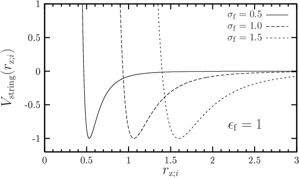
Alternatively, the Lennard-Jones potential for the interaction between a monomer and the string can be integrated out along the string axis to yield (1c),
| (2) |
where is the van der Waals radius of the string and can be considered as its effective “thickness”. It is related to the minimum distance of the string potential via
| (3) |
For convenience, we scale the string “charge” density in such a way that the minimum value of the potential is independently of , i.e., we set . Fig. 1 shows the correspondingly scaled string potential for different values of .
3 Simulational details
Polymer systems are known to possess highly nontrivial, rugged free-energy landscapes [16]. For the simulation, we have, therefore, applied generalized-ensemble Monte Carlo methods. The ground-state energies have been estimated by using various, but conceptually similar, stochastic methods such as parallel tempering, Wang–Landau, and multicanonical sampling [11, 12, 17, 13], as well as especially designed optimizing approaches like energy landscape paving, where the energy landscape is deformed irreversibly during the simulation [18, 19, 20]. The efficiency of all stochastic methods strongly depends on the conformational update set used (and, of course, on the fine-tuning of each method). If a move set is chosen reasonably well, all methods lead to comparable results in similar times. In addition, we have refined low-energy states by standard deterministic optimization techniques such as the conjugate gradient method.
For the estimation of the density of states and hence all thermodynamic quantities, we employed the Wang-Landau method [13, 21] for the determination of the multicanonical weights and performed a final production run in the multicanonical ensemble [11, 12, 17]. Independently of the values of the potential parameters, we partition the simulated energy interval into 10 000 bins in each simulation. The actual bin size hence depends on the energy range delimited by the putative ground-state energy and a fixed boundary on high energies.

As known and mentioned above, the choice of the update scheme is crucial for the efficiency of any Monte Carlo simulation in general. For conformational changes, we apply here a variety of update moves, see Fig. 2, including local crankshaft [Fig. 2(a)] and slithering-snake moves [Fig. 2(b)], as well as global spherical-cap [Fig. 2(c)] and translation moves. Sets including these steps have been found to work quite well in previous studies as well [22, 23, 24]. The crankshaft move is just a rotation of a single monomer around the virtual bond between its neighbors, or, if the monomer is an end-monomer, around the elongation of the one neighboring bond. For the slithering-snake update, we cut a monomer from one end and paste it at the other end keeping the bond vector fixed. Both updates induce small conformational changes of the whole chain, whereas the latter one enables the polymer to leave very dense, adsorbed conformations.
The spherical-cap update consists of the shift of monomers by a small constant vector keeping the bond lengths at the th monomer fixed. It hence allows for larger steps in the conformational space compared to the former local updates. The global translation update finally allows for a direct displacement of the chain relative to the string, which in the entire simulation remains fixed in the box. In any Monte Carlo step, we choose the different moves randomly with equal weight. We convinced ourselves that this provides a reasonable sampling of the conformational space of this model system on large scales as well as locally. It behaves in general not worse and for the ground-state search even better than a procedure consisting of a few global moves followed by much more local moves, whereas the ratio depends on the system size. However, such a procedure has been found to be favorable for other problems [24].
Alternative, more sophisticated update moves like bond-bridging or monomer-jump moves [25, 23, 24, 26] have not been included in our update set as they are rather time consuming and would apparently not improve the principal findings of the present study. Though, they are necessary for studying structural transitions in the dense and crystalline regime [22, 23], or for the investigation of much larger systems. In the following, we discuss the structural properties of a polymer with monomers.
4 Ground states of the system

There are two parameters in the interaction potential between the string and monomers [Eq. (1c) and Fig. 1], the van der Waals radius proportional to the effective thickness of the string, , and the adsorption strength . By varying these two parameters, we have recently constructed the complete conformational phase diagram of low-energy structures [1, 27]. By introducing suitable observables, four major structural phases have been identified. For small values of and , i.e., for very thin and weakly attracting strings, we find globular or spherical polymer droplets inclosing the string (phase Gi). In this case, the polymer structures are similar to that in bulk under poor solvent conditions. The string does not influence the shape of these structures but affects only the internal structure of the droplet.
Figure 3 shows conformations with . In Figs. 3(a) and 3(b), droplets inclosing the string are visualized. When increasing the van der Waals radius of the string, monomer–monomer bonds inside the droplet will be broken and, hence, the string is excluded from the droplet but still it is attached to it (phase Ge). The radius at which this rearrangement occurs depends on . For , i.e., where the string attraction is not significantly stronger than the monomer–monomer attraction, the transition occurs, roughly, when the diameter of the string becomes comparable to the equilibrium distance between two monomers. When further increasing the string radius, the string moves outward and the structure approaches the bulk conformation. See Figs. 3(c)–(e) for examples of conformations at different values, thus visualizing the described “process”.

Increasing at any given value of the string attraction strength , globular structures (Gi, Ge) start to deform and to lose spherical symmetry at . For , we observe a transition from phase Gi directly to the barrel phase B, which is characterized by closed, stretched conformations with cylinderlike shape wrapping around the string. In the extreme case of very strong string attraction, polymers form monolayer tubes. For , the polymer first adopts clamshell-like conformations (phase C) before it forms barrel structures in phase B. Interestingly, the evolution from spherical droplets to monolayer tubes involves the formation of distinguishable monomer layers.
For illustration, we plot in the upper row in Fig. 4 the radial distribution of monomers with respect to the string of certain low-energy structures. One finds accumulations of monomers at different distances from the string, i.e., in different layers. The position of the first layer corresponds to the van der Waals radius of the string [cp. Eq. (3), ], whereas the location of the higher-order layers is connected to the equilibrium distance between the monomers, corresponding to . In the lower row, respective structures are depicted. In Fig. 4(a), we plot the radial distribution of monomers in a conformation from phase Ge with . The emergence of different peaks in that function can be observed. A clear 3-layer structure can be identified in Fig. 4(b), where a typical conformation in phase C is shown (). In Fig. 4(c), a two-layer barrel-shaped conformation is shown () which transforms into a monolayer tube at , as depicted in Fig. 4(d). We would like to note here that, in particular, these monolayer tubes exhibit interesting similarities to other structures in nature like, for example, carbon nanotubes [1, 27, 28, 29].
5 Thermodynamics of the adsorption


Finally, we short comment on thermodynamic properties of the adsorption transition [15]. For estimating the finite-system transition temperature, we first identify peak positions in the canonical specific-heat curves, associated to the transition. In Fig. 5(a) we plot these peaks for a polymer consisting of monomers and a string with for various values of the substrate adhesion strength . In Fig. 5(b), we plot the transition temperatures corresponding to the peak positions depending on . We find an almost linear increase of the adsorption temperature with adsorption strength, a behavior which was in the same way observed in a recent study, where this transition has been studied for the same polymer model interacting with planar substrates [8].
A more adequate description of the thermodynamic behavior of small finite-size systems provides the microcanonical analysis [30, 31, 32, 33, 24, 34], based on the fact that all the relevant information about the system is encoded in its density of states . In Fig. 6(a), we plot the logarithm of this function, which is proportional to the microcanonical entropy []. The adsorption transition is represented by the convex region in the microcanonical entropy. The energetic width of this convex part is a measure for the latent heat which is nonzero for a first-order-like transition. The derivative of the microcanonical entropy with respect to the energy yields the inverse microcanonical temperature . It is plotted in Fig. 6(b) and exhibits a monotonic change in the transition region (therefore called “backbending effect”). The microcanonical transition temperature is obtained by a Maxwell construction in that region, indicated by horizontal lines in Fig. 6(b). We note, in particular, that for and , backbending does not occur. The inflection points in this energetic region indicate second-order-like transitions and belong to the transition in bulk. This agrees with previous observations that the “strength” of the first-order signal decreases with decreasing substrate adsorption strength [34]. A more detailed analysis of the structural transitions in the polymer–wire system by means of microcanonical thermodynamics will be presented in a forthcoming paper [15].
Acknowledgment
This work is supported by the Umbrella program under Grant No. SIM6 and by supercomputer time provided by the Forschungszentrum Jülich under Project Nos. jiff39 and jiff43.
References
- [1] Vogel, T. and Bachmann, M., Phys. Rev. Lett. 104 (2010) 198302.
- [2] Bachmann, M., Goede, K., Beck-Sickinger, A. G., Grundmann, M., Irbäck, A., and Janke, W., Angew. Chem. Int. Ed. 49 (2010) 9530.
- [3] Gao, M., Dai, L., and Wallace, G. G., Electroanalysis 15 (2003) 1089.
- [4] Hasan, T., Sun, Z., Wang, F., Bonaccorso, F., Tan, P. H., Rozhin, A. G., Ferrari, A. C., Adv. Mater. 21 (2009) 3874.
- [5] Milchev, A. and Binder, K., J. Chem. Phys. 114 (2001) 8610.
- [6] Bachmann, M. and Janke, W., Phys. Rev. Lett. 95 (2005) 058102.
- [7] Bachmann, M. and Janke, W., Phys. Rev. E 73 (2006) 020901(R).
- [8] Möddel, M., Bachmann, M., and Janke, W., J. Phys. Chem. B 113 (2009) 3314.
- [9] Milchev, A. and Binder, K., J. Chem. Phys. 117 (2002) 6852.
- [10] Gurevitch, I. and Srebnik, S., Chem. Phys. Lett. 444 (2007) 96.
- [11] Berg, B. A. and Neuhaus, T., Phys. Lett. B 267 (1991) 249.
- [12] Berg, B. A. and Neuhaus, T., Phys. Rev. Lett. 68 (1992) 9.
- [13] Wang, F. and Landau, D. P., Phys. Rev. Lett. 86 (2001) 2050.
- [14] Schnabel, S., Bachmann, M., and Janke, W., Phys. Rev. Lett. 98 (2007) 048103.
- [15] Vogel, T. and Bachmann, M., preprint (2011).
- [16] Janke, W., editor, Rugged Free Energy Landscapes, volume 736 of Lecture Notes in Physics, Springer, Berlin, 2008.
- [17] Janke, W., Physica A: Stat. Theor. Phys. 254 (1998) 164.
- [18] Wenzel, W. and Hamacher, K., Phys. Rev. Lett. 82 (1999)3003.
- [19] Hansmann, U. H. E., Eur. Phys. J. B 12 (1999) 607.
- [20] Hansmann, U. H. E. and Wille, L. T., Phys. Rev. Lett. 88 (2002) 068105.
- [21] Zhou, C. and Bhatt, R. N., Phys. Rev. E 72 (2005) 025701(R).
- [22] Schnabel, S., Vogel, T., Bachmann, M., and Janke, W., Chem. Phys. Lett. 476 (2009) 201.
- [23] Schnabel, S., Bachmann, M., and Janke, W., J. Chem. Phys. 131 (2009) 124904.
- [24] Taylor, M. P., Paul, W., and Binder, K., J. Chem. Phys. 131 (2009) 114907.
- [25] Deutsch, J. M., J. Chem. Phys. 106 (1997) 8849.
- [26] Reith, D. and Virnau, P., Comp. Phys. Comm. 181 (2010) 800.
- [27] Vogel, T. and Bachmann, M., Phys. Proc. 4 (2010) 161.
- [28] Vogel, T., Mutat, T., Adler, J., and Bachmann, M., Accurate modeling approach for the structural comparison between monolayer polymer tubes and single-walled nanotubes, Phys. Proc., in press (2011).
- [29] Vogel, T., Mutat, T., Adler, J., and Bachmann, M., Morphological similarities of carbon nanotubes and polymers adsorbed on nanowires, preprint (2011).
- [30] Gross, D. H. E., Microcanonical Thermodynamics, World Scientific, Singapore, 2001.
- [31] Junghans, C., Bachmann, M., and Janke, W., Phys. Rev. Lett. 97 (2006) 218103.
- [32] Junghans, C., Bachmann, M., and Janke, W., J. Chem. Phys. 128 (2008) 085103.
- [33] Junghans, C., Bachmann, M., and Janke, W., EPL (Europhys. Lett.) 87 (2009) 40002.
- [34] Möddel, M., Bachmann, M., and Janke, W., Phys. Chem. Chem. Phys. 12 (2010) 11548.