From Weak Lensing to non-Gaussianity via Minkowski Functionals

Dipak Munshi Affiliation: School of Physics and Astronomy, Cardiff University, Queen’s Buildings, 5 The Parade, Cardiff, CF24 3AA, UK Ludovic van Waerbeke Affiliation: Department of Physics & Astronomy, University of British Columbia, 6224 Agricultural Road, Vancouver, B.C. V6T 1Z1, Canada Joseph Smidt Affiliation: Department of Physics and Astronomy, University of California, Irvine, CA 92697 Peter Coles Affiliation: School of Physics and Astronomy, Cardiff University, Queen’s Buildings, 5 The Parade, Cardiff, CF24 3AA, UK

August 24, 2026, Revision: 0.9

Abstract

We present a new harmonic-domain based approach for extracting morphological information, in the form of Minkowski Functionals (MFs), from weak lensing (WL) convergence maps. Using a perturbative expansion of the MFs, which is expected to be valid for the range of angular scales probed by most current weak-lensing surveys, we show that the study of three generalized skewness parameters is equivalent to the study of the three MFs defined in two dimensions. We then extend these skewness parameters to three associated skew-spectra which carry more information about the convergence bispectrum than their one-point counterparts. We discuss various issues such as noise and incomplete sky coverage in the context of estimation of these skew-spectra from realistic data. Our technique provides an alternative to the pixel-space approaches typically used in the estimation of MFs, and it can be particularly useful in the presence of masks with non-trivial topology. Analytical modeling of weak lensing statistics relies on an accurate modeling of the statistics of underlying density distribution. We apply three different formalisms to model the underlying dark-matter bispectrum: the hierarchical ansatz, halo model and a fitting function based on numerical simulations; MFs resulting from each of these formalisms are computed and compared. We investigate the extent to witch late-time gravity-induced non-Gaussianity (to which weak lensing is primarily sensitive) can be separated from primordial non-Gaussianity and how this separation depends on source redshift and angular scale.

Keywords:

: Cosmology– Weak-Lensing – Methods: analytical, statistical, numerical

1 Introduction

Since the first measurements were published (Beacon, Refregier & Ellis, 2000; Wittman et al, 2000; Kaiser, Wilson & Luppino, 2000; Waerbeke et al, 2000) there has been tremendous progress in the field of weak gravitional lensing, regarding analytical modelling, as well as technical specification and control of systematics in observational surveys. Ongoing and planned weak lensing surveys (see Munshi et al. (2008) for a review) such as the CFHT¹¹ 1 http://www.cfht.hawai.edu/Sciences/CFHLS/ Legacy Survey, Pan-STARRS²² 2 http://pan-starrs.ifa.hawai.edu/, the Dark Energy Survey³³ 3 https://www.darkenergysurvey.org/, and, further in the future, the Large Synoptic Survey Telescope⁴⁴ 4 http://www.lsst.org/llst_home.shtml, JDEM⁵⁵ 5 http://jdem.gsfc.nasa.gov/ and Euclid ⁶⁶ 6 http://http://sci.esa.int/euclid will map the cosmological distribution of dark matter and probe the properties of dark energy in unprecedented detail. Owing to the greater sky coverage, tighter control on systematics and increased number-density of source galaxies it will be soon possible to extract higher-order statistics (i.e. beyond the two-point correlation function), such as multispectra; see e.g. Pen et al. (2003). Non-linearity induced by gravitational effects is generally used to break the degeneracy between the amplitude of matter power spectrum $\sigma_{8}$ and the matter density parameter $\Omega_{M}$ ; three-point statistics such as the bispectrum (the three-point multispectrum) are the best studied statistics for this purpose (Villumsen, 1996; Jain & Seljak, 1997). Weak lensing can therefore play an important role in breaking degeneracies, which makes it an ideal complement to Cosmic Microwave Background (CMB) studies and studies involving large scale structure (LSS) surveys.

Two-point statistics, principally the power spectrum, of density perturbations remain the most frequently used statistical tool for many cosmological studies. Weak lensing surveys probe the non-linear regime and are therefore sensitive to non-Gaussian signatures which can not be probed using two-point statistics. The statistics of shear or convergence probe the statistics of underlying mass distribution in an unbiased way (Jain, Seljak & White, 2000; Munshi & Jain, 2001; Munshi, 2000; Munshi & Jain, 2000; Munshi & Jain, 2001; Valageas, 2000; Munshi & Valageas, 2005; Valageas, Barber, & Munshi, 2004; Valageas, Munshi & Barber, 2005; Takada & White, 2003; Takada & Jain, 2004), but are very sensitive to nonlinear evolution driven by gravitational clustering. A number of analytical schemes, from perturbative calculations to halo models have therefore been employed to model weak lensing statistics Fry (1984); Schaeffer (1984); Bernardeau & Schaeffer (1992); Szapudi & Szalay (1993); Szapudi & Szalay (1997); Munshi et al (1999); Munshi, Coles & Melott (1999a); Munshi, Coles & Melott (1999b); Munshi, Melott & Coles (1999); Munshi & Coles (2000); Munshi & Coles (2002); Munshi & Coles (2003); Cooray & Seth (2002)). In addition to studying the statistics in projection on the sky, they have also been studied in three dimensions using photometric redshifts. It has been demonstrated that this approach can tighten observational constraints on such quantities as the neutrino mass and the dark energy equation of state parameter(Heavens, 2003; Heavens et al., 2000; Heavens et al, 2006; Heavens, Kitching & Verde, 2007; Castro et al, 2005; Kitching et al., 2008). Tomographic techniques have also been employed as an intermediate strategy between projected surveys and 3D mapping (Hu, 1999; Takada & Jain, 2004; Takada & Jain, 2003; Semboloni et al, 2008).

Refer to caption — Figure 1: The power spectrum is plotted as a function of the harmonics $l$ in the left panel. A WMAP7 background cosmology is used. The results are displayed for three different source redshifts $z_{s}=1.5$ , $1.0$ and $0.5$ . The cosmological parameters are $\Gamma=0.1956$ , $\Omega=0.279$ , $\Lambda=0.721$ and $\sigma_{8}=0.817$ respectively. The dot-dashed curve shows predictions from the halo model for the same WMAP7 background cosmology and for the source redshift $z_{s}=1$ . The diagonal entries of the bi-spectrum are plotted as a function of the harmonics $l$ in the right panel. The results are for $z_{s}=1.0$ . Two different approaches are persued in computation of the bispectrum. The bispectrum results based on extnsions of perturbation theory Eq.(43) are plotted using solid lines, the halo model predictions i.e. Eq.(40) are shown using dashed lines.

Minkowski Functionals (MFs) are morphological descriptors that are commonly used in many cosmological contexts. They can be defined for both 2D (projected) and 3D (redshift) data, and have been used to probe non-Gaussianity in CMB data (Natoli et al., 2010; Komatsu et al., 2003; Eriksen et al., 2004), weak lensing surveys (Matsubara & Jain, 2001; Sato et al., 2001; Taruya et al., 2002) and galaxy surveys (Gott, Melott & Dickinson, 1986; Coles, 1988; Gott et al., 1989; Melott et al., 1989; Moore et al., 1992; Gott et al., 1992; Rhodas, Gott & Postman, 1994; Canavezes et al., 1998; Park et al., 2005; Hikage et al., 2008; Hikage et al., 2006; Hikage, Taruya & Suto, 2003; Hikage et al., 2002). Unlike the multispectra, discussed above the topological descriptors carry information of all orders (in a statistical sense). In the context of CMB studies, the MFs are used to probe primordial non-Gaussianity. For large scale structure studies using projected or redshift galaxy surveys, the non-Gaussianity probed is mainly that which is induced by gravity. While galaxy surveys suffer from uncertainties relating to the nature of galaxy bias, weak lensing surveys will provide an unbiased probe to probe the clustering of dark matter. The MFs will be an important tool in this direction, along with other statistics that can be used to probe non-Gaussianity to break the parameter-space that are unavoidable when the power spectrum alone is used.

This paper is organized as follows. In §2 we review the formalism of Minkowski Functionals. In §3 we link the statistics of weak lensing convergence and the underlying density distribution. In §4 we introduce the concept of generalized skew-spectra and show how these power spectra can be used to study the Minkowski Functionals. In §5 we review the analytical models that are typically used for modelling of dark matter clustering.

2 Formalism

The MFs are well-known morphological descriptors which are used in the study of random fluctuation fields fields. Morphological properties are defined to be those properties that remain invariant under rotation and translation; see Hadwiger (1959) for a more formal introduction. They are defined over an excursion set $\Sigma$ for a given threshold $\nu$ . The three MFs that are defined for two dimensional (2D) studies can be expressed, following the notations of (Hikage et al., 2008), as:

V_{0}(\nu)=\int_{\Sigma}da;\quad V_{1}(\nu)={1\over 4}\int_{\partial\Sigma}dl;\quad V_{2}(\nu)={1\over 2\pi}\int_{\partial\Sigma}{\cal K}dl

(1)

Here $da$ , $dl$ are surface are and line elements for the excursion set $\Sigma$ and its boundary $\partial\Sigma$ respectively. The MFs $V_{k}(\nu)$ correspond to the area of the excursion set $\Sigma$ , the length of its boundary $\partial\Sigma$ as well as the integral of curvature $\cal K$ along its boundary which is also related to the genus $g$ and hence the Euler characteristics $\chi$ .

In our analysis we will consider a smoothed random field $\kappa({\hat{\Omega}})$ , with mean $\langle\kappa({\hat{\Omega}})\rangle=0$ and variance $\sigma_{0}^{2}=\langle\kappa^{2}({\hat{\Omega}})\rangle$ ; for the time being $\kappa$ is a generic 2D weakly non-Gaussian random field defined on the sky although we will introduce more specific examples later on. The spherical harmonic decomposition, using $Y_{lm}({\hat{\Omega}})$ as basis functions, $\kappa({\hat{\Omega}})=\sum_{lm}\kappa_{lm}Y_{lm}({\hat{\Omega}})$ , can be used to define the power spectrum ${\cal C}_{l}$ using $\langle\kappa_{lm}\kappa^{*}_{l^{\prime}m^{\prime}}\rangle={\cal C}_{l}\delta_{ll^{\prime}}\delta_{mm^{\prime}}$ which is a sufficient statistical characterization of a Gaussian field. For a non-Gaussian field, higher-order statistics such as the bi- or tri-spectrum can describe the resulting mode-mode coupling. An alternative to this laborious expansion in multispectra, topological measures such as the Minkowski functionals can be employed to quantify deviations from Gaussianity and it can be shown that the information content in both descriptions is the same. At leading order the MFs can be constructed completely from the knowledge of the bispectrum alone. We will be studying the MFs defined over the surface of the celestial sphere but equivalent results can be obtained in 3D using Fourier decomposition (Munshi 2010, in preparation). The behaviour of the MFs for a random Gaussian field is well known and is given by Tomita’s formula (Tomita, 1986). The MFs are denoted by $V_{k}(\nu)$ for a threshold $\nu=\kappa/\sigma_{0}$ , where $\sigma^{2}_{0}=\langle\kappa^{2}\rangle$ can be decomposed into two different contributions, Gaussian ( $V^{G}_{k}(\nu)$ ) and non-Gaussian ( $\delta V_{k}(\nu)$ ), i.e. $V_{k}(\nu)=V_{k}^{G}(\nu)+\delta V_{k}(\nu)$ . From our perspective we will be more interested in the non-Gaussian contribution, i.e. $\delta V_{k}(\nu)$ . We will further separate out an amplitude $A$ in the expressions of both of these contributions which depend only on the power spectrum of the perturbation through $\sigma_{0}$ and $\sigma_{1}$ (see e.g. Hikage et al. (2008)):

	$\displaystyle V^{G}_{k}(\nu)=A\exp\left(-{\nu^{2}\over 2}\right)H_{k-1};\quad\quad\delta V_{k}(\nu)=A\exp\left(-{\nu^{2}\over 2}\right)\left[\delta V_{k}^{(2)}(\nu)\sigma_{0}+\delta V_{k}^{(3)}(\nu)\sigma_{0}^{2}+\delta V_{k}^{(4)}(\nu)\sigma_{0}^{3}+\cdots\right]$		(2)
	$\displaystyle\delta V_{k}^{(2)}(\nu)=\left[\left\{{1\over 6}S^{(0)}H_{k+2}(\nu)+{k\over 3}S^{(1)}H_{k}(\nu)+{k(k-1)\over 6}S^{(2)}H_{k-2}(\nu)\right\}\right];\quad\quad A={1\over(2\pi)^{(k+1)/2}}{\omega_{2}\over\omega_{2-k}\omega_{k}}\left(\sigma_{1}\over\sqrt{2}\sigma_{0}\right)^{k}.$		(3)

The constant $\omega_{k}$ introduced above is the volume of the unit sphere in $k$ dimensions, i.e. $w_{k}=\pi^{k/2}/\Gamma(k/2+1)$ ; in 2D we will only need $\omega_{0}=1$ , $\omega_{1}=2$ and $\omega_{2}=\pi$ . The lowest-order Hermite polynoimals $H_{k}(\nu)$ are listed below. As mentioned previously, the expressions consist of two distinct contributions. The part which does not depend on the three different skewness paramters $S^{(0)},S^{(1)},S^{(2)}$ signifies the MFs for a Gaussian random field. The other contribution $\delta V_{k}(\nu)$ represents the departure from the Gaussian statistics and depends on the generalised skewness parameters defined in Eq.(5) and Eq.(2). We have expanded the total non-Gaussian contribution into perturbation series in $\sigma_{0}$ . While the lowest order terms $\delta V_{k}^{(2)}(\nu)$ are determined by various one-point moments related to the bispectrum the next-to- leading-order terms $\delta V_{k}^{(3)}(\nu)$ are connected to similar one-point moments related to trispectrum (also known as the kurtosis). In projected surveys, even for relatively small angular smoothing scales, the leading order terms are sufficient to describe the non-Gaussian departures in the smoothed convergence field $\kappa(\theta_{s})$ .

	$\displaystyle H_{-1}(\nu)=\sqrt{\pi\over 2}e^{\nu^{2}/2}{\rm erfc}\left(\nu\over\sqrt{2}\right);\quad H_{0}(\nu)=1,\quad H_{1}(\nu)=\nu,{}$
	$\displaystyle H_{2}(\nu)=\nu^{2}-1,\quad H_{3}(\nu)=\nu^{3}-3\nu,\quad\quad H_{4}(\nu)=\nu^{4}-6\nu^{2}+3.{}$
	$\displaystyle H_{n}(\nu)=(-1)^{n}\exp\left({\nu^{2}\over 2}\right){d\over d\nu^{n}}\exp\left({-\nu^{2}\over 2}\right)$		(4)

The various quantities $\sigma_{j}$ that appear in Eq.(3) can be expressed in terms of the power spectra ${\cal C}_{l}$ and the shape of the observational beam $b_{l}$ . The moment $\sigma_{0}$ is a special case for which $\sigma_{0}^{2}$ corresponds to the variance. The quantities $\sigma_{1}$ , $\sigma_{2}$ are natural generalisations of variance, with increasing $j$ corresponding to increase weight towards higher harmonics $\sigma_{j}^{2}={1\over 4\pi}\sum(2l+1)[l(l+1)]^{j}{\cal C}_{l}b_{l}^{2}$ . The variance that will mostly be used are $\sigma_{0}^{2}=\langle\kappa^{2}\rangle$ and $\sigma_{1}^{2}=\langle(\nabla\kappa)^{2}\rangle$ .

The real-space expressions for the triplets of skewness $S^{(i)}$ are given below. These are natural generalisations of the ordinary skewness $S^{0}$ that is used in many cosmological studies. They all are cubic statistics but are constructed from different cubic combinations:

S^{(0)}\equiv{S^{(\kappa^{3})}\over\sigma_{0}^{4}}={\langle\kappa^{3}\rangle\over\sigma_{0}^{4}};\quad S^{(1)}\equiv-{3\over 4}{S^{(\kappa^{2}\nabla^{2}\kappa)}\over\sigma_{0}^{2}}=-{3\over 4}{\langle\kappa^{2}\nabla^{2}\kappa\rangle\over\sigma_{0}^{2}\sigma_{1}^{2}};\quad S^{(2)}\equiv S^{(\nabla\kappa\cdot\nabla\kappa\nabla^{2}\kappa)}=-{3}{\langle(\nabla\kappa).(\nabla\kappa)(\nabla^{2}\kappa)\rangle\over\sigma_{1}^{4}}.

(5)

The expressions in the harmonic domain are more useful in the context of CMB studies where we will be recovering them from a masked sky using analytical tools that are commonly used for power spectrum analysis. The skewness parameter $S^{(1)}$ is constructed from the product field $\kappa^{2}$ and $\nabla^{2}f$ , whereas skewness parameter $S^{(2)}$ relies on the construction of $[\nabla\kappa\cdot\nabla\kappa]$ and $\nabla^{2}\kappa$ . By construction, the skewness parameter $S^{(2)}$ has the highest weight at high $l$ modes and $S^{(0)}$ has the lowest weights on high $l$ modes. The expressions in terms of the bispectrum $B_{l_{1}l_{2}l_{3}}$ (see Eq.(12) for defintion) take the following form (see e.g. Hikage et al. (2008)):

	$\displaystyle S^{(\kappa^{3})}={1\over 4\pi}\sum_{l_{i}}{\cal B}_{l_{1}l_{2}l_{3}}I_{l_{1}l_{2}l_{3}}$		(6)
	$\displaystyle S^{(\kappa^{2}\nabla^{2}\kappa)}=-{1\over 12\pi}\sum_{l_{i}}{}\Big[{l_{1}(l_{1}+1)+l_{2}(l_{2}+1)+l_{3}(l_{3}+1)}\Big]{\cal B}_{l_{1}l_{2}l_{3}}I_{l_{1}l_{2}l_{3}}$		(7)
	$\displaystyle S^{(\nabla\kappa\cdot\nabla\kappa\nabla^{2}\kappa)}={1\over 4\pi}\sum_{l_{i}}{}\Big[[l_{1}(l_{1}+1)+l_{2}(l_{2}+1)-l_{3}(l_{3}+1)]l_{3}(l_{3}+1)+{\rm cyc.perm.}\Big]{\cal B}_{l_{1}l_{2}l_{3}}I_{l_{1}l_{2}l_{3}}W_{l_{1}}W_{l_{2}}W_{l_{3}}$		(8)
	$\displaystyle I_{l_{1}l_{2}l_{3}}=\sqrt{(2l_{1}+1)(2l_{2}+1)(2l_{3}+1)\over 4\pi}\left(\begin{array}[]{ c c c }l_{1}&l_{2}&l_{3}\\ 0&0&0\end{array}\right).$

The bispectrum $B_{l_{1}l_{2}l_{3}}$ used here defines the three-point correlation function in the harmonic domain. A reduced bispectrum $b_{l_{1}l_{2}l_{3}}$ can also be defined which can directly be linked to the flat-sky expressions.

\langle\kappa_{l_{1}m_{1}}\kappa_{l_{2}m_{2}}\kappa_{l_{3}m_{3}}\rangle_{c}=\left(\begin{array}[]{ c c c }l_{1}&l_{2}&l_{3}\\ m_{1}&m_{2}&m_{3}\end{array}\right){\cal B}_{l_{1}l_{2}l_{3}};\quad\quad{\cal B}_{l_{1}l_{2}l_{3}}=I_{l_{1}l_{2}l_{3}}b_{l_{1}l_{2}l_{3}}.

(12)

The expressions for the MFs in Eq.(3) depend on the one-point cumulants $S^{(i)}$ . However it is possible to define power spectra associated with each of these skewnesses following a procedure developed in Munshi & Heavens (2010). This will mean we can also associate a power spectrum with $V_{k}^{(3)}$ which will generalize the concept of MFs in a scale-dependent way. The power spectrum that we associate with MFs will have the same correspondence with various skew-spectra $S^{(i)}_{l}$ as the MFs have with one-point cumulants or $S^{(0)}$ . The power spectra so defined will however have more power to distinguish various models of non-Gaussianity. This is one of the main motivations behind generalising the concept of MFs, each of which is a number, to a power spectrum, which contains scale information.

The series expansion for the MFs can be extended beyond the level of the bispectrum; the next-to-leading-order corrections terms are related to trispectra of the original fields and various derivatives constructed from them using differential operations such as $\nabla\cdot\nabla,\nabla^{2}$ . These corrections are expected to be sub-dominant in the context of CMB studies for the entire range of angular scales being probed.

The results here correspond to analysis of convergence maps, which are spin- $0$ objects. It is possible to extend these results to spin-2 fields. Such results will be interesting for analysis of weak lensing shear and flexions, but a detailed analysis will be presented elsewhere.

3 Convergence power spectrum and bispectrum

The convergence $\kappa({\hat{\Omega}},r_{s})$ can be treated as a line-of-sight projection of the density contrast $\delta({\hat{\Omega}},r)$ along the direction ${\hat{\Omega}}$ ( $r$ is comoving radial distance) out to a source redshift $z_{s}(r_{s})$ with a redshift-dependent weight function $\omega(r,r_{s})$ :

\kappa({\hat{\Omega}},r_{s})=\int_{0}^{r_{s}}\,dr\,w(r,r_{s})\,\delta({\hat{\Omega}},r);\quad\omega(r,r_{s})={3\over 2a}{H_{0}^{2}\over c^{2}}\Omega_{M}{d_{A}(r-r_{s})\over d_{A}(r)d_{A}(r_{s})};\quad r_{s}={\rm min}(r_{1},r_{2}).

(13)

The weight functions $\omega(r)$ for weak lensing depend on the angular diameter distance $d_{A}(r)$ , Hubble constant $H_{0}$ , matter density parameter $\Omega_{M}$ and the scale factor of the Universe $a=1/(1+z)$ at a redshift $z$ . The angular diameter distance $d_{A}(r)$ is linked to the total matter content $\Omega_{0}$ and the Hubble constant $H_{0}$ , i.e. $d_{A}(r)={\rm K}^{-1/2}\sin({\rm K}^{-1/2}r),\;{\rm K}^{-1/2}\sinh((-{\rm K})^{-1/2}r),\;r$ for open, closed and flat Universes; here ${\rm K}=(\Omega_{0}-1)H_{0}^{2}$ . We will consider the projected cross-power spectra $C_{l}$ that depend on two different redshift $z_{1}$ and $z_{2}$ which is a function of the underlying matter power spectra $P_{\delta}(k,r)$ which, in the small-angle approximation (Limber, 1954), can be expressed as (Kaiser, 1992):

{\cal C}_{l}=\int_{0}^{r_{s}}\,dr\,\,{w^{2}(r;r_{s})\over d^{2}_{A}(r)}\,P_{\delta}\left({l\over d_{A}(r)},r\right);\quad

(14)

Analytical modelling of the convergence bispectrum ${\cal B}$ depends on modelling of the underlying matter bispectrum $B_{\delta}$ :

{\cal B}_{l_{1}l_{2}l_{3}}=I_{l_{1}l_{2}l_{3}}\int_{0}^{r_{s}}dr\,{w^{3}(r,r_{s})\over d^{4}_{A}(r)}\,B_{\delta}\left({l_{1}\over d_{A}(r)},{l_{2}\over d_{A}(r)},{l_{3}\over d_{A}(r)}\right);\quad

(15)

we will discuss the analytical models we use to construct $B_{\delta}$ in later sections.This equation can also be used to express the reduced bispectrum $b_{l_{1}l_{2}l_{3}}$ introduced before in Eq.(12). Estimation of individual modes of the bispectrum defined by specific choice of the triplets $(l_{1},l_{2},l_{3})$ is difficult when the data are noisy, but it is possible to extract the cross-correlation of product maps $\kappa^{2}({\hat{\Omega}})$ against $\kappa({\hat{\Omega}})$ . If we denote the harmonics of the product map $\kappa^{2}({\hat{\Omega}})$ as $\kappa_{lm}^{(2)}=\int\,d{\hat{\Omega}}\,Y^{*}_{lm}({\hat{\Omega}})\kappa^{2}({\hat{\Omega}})$ and similarly $\kappa_{lm}=\int\,d{\hat{\Omega}}\,Y^{*}_{lm}({\hat{\Omega}})\kappa({\hat{\Omega}});$ then the associated power spectrum is constructed as ${\cal C}_{l}^{(2,1)}={1\over 2l+1}\sum_{l}{\rm Re}(\kappa_{lm}^{(2)}\kappa_{lm}^{(1)})$ is called the skew-spectrum (Cooray, 2001). We will next generalize the concept of skew-spectrum and introduce a set of generalized skew-spectrum that can be used to construct the Minkowski Functionals at the lowest level of non-Gaussianity.

4 The triplets of skew-spectra and lowest-order corrections to Gaussian MFs

The skew-spectra are cubic statistics that are constructed by cross-correlating two different fields. One of the field used is a composite field typically a product of two maps either in its original form or constructed by means of relevant differential operations. The second field will typically be a single field but may be constructed by applying various differential operators. All three skewnesses contribute to the three MFs that we will consider in 2D.

The first of the skew-spectra was studied by (Cooray, 2001) and was later generalized by Munshi & Heavens (2010) and is related to commonly used skewness. The skewness in this case is constructed by cross-correlating the squared map $[\kappa^{2}({\hat{\Omega}})]$ with the original map $[\kappa({\hat{\Omega}})]$ . The second skew-spectrum is constructed by cross-correlating the squared map $[\kappa^{2}({\hat{\Omega}})]$ against $[\nabla^{2}\kappa({\hat{\Omega}})]$ . Analogously, the third skew-spectrum represents the cross-spectra that can be constructed using $[\nabla\kappa({\hat{\Omega}})\cdot\nabla\kappa({\hat{\Omega}})]$ and $[\nabla^{2}\kappa({\hat{\Omega}})]$ maps.

	$\displaystyle S_{l}^{(0)}\equiv{1\over 12\pi\sigma_{0}^{4}}S_{l}^{(\kappa^{2},\kappa)}\equiv{1\over 12\pi\sigma_{0}^{4}}{1\over 2l+1}\sum_{m}{\rm Real}([\kappa]_{lm}[\kappa^{2}]^{*}_{lm})={1\over 12\pi\sigma_{0}^{4}}\sum_{l_{1}l_{2}}{\cal B}_{ll_{1}l_{2}}J_{ll_{1}l_{2}}W_{l}W_{l_{1}}W_{l_{2}}$		(16)
	$\displaystyle S_{l}^{(1)}\equiv{1\over 16\pi\sigma_{0}^{2}\sigma_{1}^{2}}S_{l}^{(\kappa^{2},\nabla^{2}\kappa)}\equiv{1\over 16\pi\sigma_{0}^{2}\sigma_{1}^{2}}{1\over 2l+1}\sum_{m}{\rm Real}([\nabla^{2}\kappa]_{lm}[\kappa^{2}]^{*}_{lm}){}$
	$\displaystyle\quad\quad={1\over 16\pi\sigma_{0}^{2}\sigma_{1}^{2}}\sum_{l_{i}}\Big[{l(l+1)+l_{1}(l_{1}+1)+l_{2}(l_{2}+1)}\Big]{\cal B}_{ll_{1}l_{2}}J_{ll_{1}l_{2}}W_{l}W_{l_{1}}W_{l_{2}}$		(17)
	$\displaystyle S_{l}^{(2)}\equiv{1\over 8\pi\sigma_{1}^{4}}S_{l}^{(\nabla\kappa\cdot\nabla\kappa,\nabla^{2}\kappa)}\equiv{1\over 8\pi\sigma_{1}^{4}}{1\over 2l+1}\sum_{m}{\rm Real}([\nabla\kappa\cdot\nabla\kappa]_{lm}[\nabla^{2}\kappa]^{*}_{lm}){}$
	$\displaystyle\quad\quad={1\over 8\pi\sigma_{1}^{4}}\sum_{l_{i}}{}\Big[[l(l+1)+l_{1}(l_{1}+1)-l_{2}(l_{2}+1)]l_{2}(l_{2}+1)+{\rm cyc.perm.}\Big]{\cal B}_{ll_{1}l_{2}}J_{ll_{1}l_{2}}W_{l}W_{l_{1}}W_{l_{2}}$		(18)
	$\displaystyle J_{l_{1}l_{2}l_{3}}\equiv{I_{l_{1}l_{2}l_{3}}\over 2l_{3}+1}=\sqrt{(2l_{1}+1)(2l_{2}+1)\over(2l_{3}+1)4\pi}\left(\begin{array}[]{ c c c }l_{1}&l_{2}&l_{3}\\ 0&0&0\end{array}\right).$
	$\displaystyle S^{(i)}=\sum_{l}(2l+1)S^{(i)}_{l}$		(22)
	$\displaystyle\sigma_{j}^{2}={1\over 4\pi}\sum_{l}(2l+1)[l(l+1)]^{j}{\cal C}_{l}W_{l}^{2}$		(23)

This set of equations constitutes one of the main results of this paper. The matrices here denote the Wigner- $3j$ symbols, $W_{l}$ represents the smoothing window, e.g. a top hat, Gaussian or some form of compensated filter. Each of these spectra probes the same bispectrum $B_{ll_{1}l_{2}}$ with different weights for individual triplets of modes that specify the bispectrum $(l,l_{1}l_{2})$ and define a triangle in the harmonic domain. The skew spectra is summed over all possible configurations of the bispectrum keeping one of its sides at a fixed $l$ . For each individual choice of $l$ we can compute the skew-spectrum $S_{l}^{(i)}$ relatively straightforwardly. by constructing the relevant maps in real space (either by algebraic or differential operation) and then cross-correlating them in the multipole domain. Issues related to mask and noise will be dealt with in later sections, where we will show that, even in the presence of a mask, the computed skew spectra can be inverted to give a unbiased estimate of all-sky skew-spectra. Presence of noise will only affect the scatter. We have explicitly displayed the experimental beam $b_{l}$ in all our expressions.

To derive the above expressions, we first express the spherical harmonic expansion of the fields $[\nabla^{2}\kappa({\hat{\Omega}})]$ , $[\nabla\kappa({\hat{\Omega}})\cdot\nabla\kappa({\hat{\Omega}})]$ and $[\kappa^{2}({\hat{\Omega}})]$ in terms of the harmonics of the original fields $\kappa_{lm}$ . These expressions involve the 3j functions as well as factors that depend on various $l_{i}$ dependent weight factors.

	$\displaystyle[\nabla^{2}\kappa({\hat{\Omega}})]_{lm}=\int~d{\hat{\Omega}}~Y^{*}_{lm}({\hat{\Omega}})~[\nabla^{2}\kappa({\hat{\Omega}})]=-l(l+1)\kappa_{lm}{}$
	$\displaystyle[\kappa^{2}({\hat{\Omega}})]_{lm}=\int~d{\hat{\Omega}}~Y^{*}_{lm}({\hat{\Omega}})~[\kappa^{2}({\hat{\Omega}})]=\sum_{l_{i}m_{i}}(-1)^{m}\kappa_{l_{1}m_{1}}\kappa_{l_{2}m_{2}}I_{l_{1}l_{2}l}\left(\begin{array}[]{ c c c }l_{1}&l_{2}&l\\ m_{1}&m_{2}&-m\end{array}\right).{}$
	$\displaystyle[\nabla\kappa({\hat{\Omega}})\cdot\nabla\kappa({\hat{\Omega}})]_{lm}=\int d{\hat{\Omega}}Y^{}_{lm}({\hat{\Omega}})[\nabla\kappa({\hat{\Omega}})\cdot\nabla\kappa({\hat{\Omega}})]=\sum_{l_{i}m_{i}}\kappa_{l_{1}m_{1}}\kappa_{l_{2}m_{2}}\int~d{\hat{\Omega}}~Y^{}_{lm}({\hat{\Omega}})~[\nabla Y_{l_{1}m_{2}}({\hat{\Omega}})\cdot\nabla Y_{l_{2}m_{2}}({\hat{\Omega}})]$		(27)
	$\displaystyle\quad\quad\quad={1\over 3}\sum_{l_{i}m_{i}}[l_{1}(l_{1}+1)+l_{2}(l_{2}+1)-l(l+1)]\int d{\hat{\Omega}}Y^{*}_{lm}({\hat{\Omega}})Y_{l_{1}m_{1}}({\hat{\Omega}})Y_{l_{2}m_{2}}({\hat{\Omega}}){}$
	$\displaystyle\quad\quad\quad={1\over 3}\sum_{l_{i}m_{i}}(-1)^{m}[l_{1}(l_{1}+1)+l_{2}(l_{2}+1)-l(l+1)]\kappa_{l_{1}m_{1}}\kappa_{l_{2}m_{2}}I_{l_{1}l_{2}l}\left(\begin{array}[]{ c c c }l_{1}&l_{2}&l\\ m_{1}&m_{2}&-m\end{array}\right).$

We can define the power spectrum associated with the MFs through the following third order expression:

V_{k}^{(3)}=\sum_{l}[V_{k}]_{l}(2l+1)={1\over 6}\sum_{l}(2l+1)\left\{S^{(0)}_{l}H_{k}(\nu)+{k\over 3}S^{(1)}_{l}H_{k-1}(\nu)+{k(k-1)\over 6}S^{(2)}_{l}H_{k-2}(\nu)+\cdots\right\}.

(31)

The three skewnesses thus define triplets of Minkowski Functionals. At the level of two-point statistics, in the harmonic domain, we have three power-spectra associated with MF $V_{k}^{(3)}$ that depend on the three skew-spectra we have defined. We will show later in this paper that the fourth order correction terms too have a similar form with an additional monopole contribution that can be computed from the lower order one-point terms in a similar way as the three skewness defined here. The result presented here is important and implies that we can study the contributions to each of the MFs $v_{k}(\nu)$ as a function of harmonic mode $l$ . This is especially significant result as various form of non-Gaussianity will have different $l$ dependence and so can potentially be distinguished from each other using this approach. The ordinary MFs add contributions from all individual $l$ modes and hence have less power in differentiating various contributing sources of non-Gaussianity. This is one of main motivations to extend the concept of MFs (single numbers) to one-dimensional objects similar to power spectrum.

It is worth pointing out that the skewness and generalized skewness parameters are relatively insensitive to the background cosmology but quite sensitive to the underlying model of non-Gaussianity. The main dependence on cosmology typically results from the normalization coefficients such as $\sigma_{0}$ and $\sigma_{1}$ which are determined the power spectrum of the convergence $\kappa$ .

In real space the skew-spectra can be defined through these correlation functions:

S^{(0)}({\hat{\Omega}}_{1},{\hat{\Omega}}_{2})\equiv\langle\kappa^{2}({\hat{\Omega}}_{1}))\kappa({\hat{\Omega}}_{2})\rangle;\quad S^{(1)}({\hat{\Omega}}_{1},{\hat{\Omega}}_{2})\equiv\langle\kappa^{2}({\hat{\Omega}}_{1})\nabla^{2}\kappa({\hat{\Omega}}_{2})\rangle;\quad S^{(2)}({\hat{\Omega}}_{1},{\hat{\Omega}}_{2})\equiv\langle\nabla\kappa({\hat{\Omega}}_{1})\cdot\nabla\kappa({\hat{\Omega}}_{1})\nabla^{2}\kappa({\hat{\Omega}}_{2})\rangle

(32)

Although we have adopted a harmonic approach these correlations can equivalently be used to probe MFs especially for smaller surveys.

5 Modelling the primordial and gravity-induced bispectrum

s It is clear that we need accurate analytical modeling of dark matter clustering for prediction of weak lensing statistics, but in general there is no definitive analytical theory for handling gravitational clustering in the highly nonlinear regime. On larger scales, where the density field is only weakly nonlinear, perturbative treatments are known to be valid. For a phenomenological statistical description of dark matter clustering in collapsed objects on nonlinear scales, typically the halo model (Cooray & Seth, 2002) is used. We will be using the Halo Model in our study, but an alternative to the Halo Model approach on small scales is to employ various ansatze which trace their origin to field-theoretic techniques. Here we provide a quick summary of some of the analytical prescriptions that can be used to model non-linear clustering. We will also provide a brief description of various models of primordial non-Gaussianity arising from variants of the inflationary universe scenario.

5.1 Hierarchical ansatz

The hierarchical ansatz has been used for many weak lensing related work, where the higher-order correlation functions are constructed from the two-point correlation functions. Assuming a tree model for the matter correlation hierarchy (typically used in the highly non-linear regime) one can write the most general case, the $N$ point correlation function, $\langle\delta({\bf r_{1}})\dots\delta({\bf r_{n}})\rangle_{c}=\xi_{N}^{\delta}({\bf r}_{1},\dots,{\bf r}_{n})$ as a product of two-point correlation functions $\langle\delta({\bf r}_{i})\delta({\bf r}_{j})\rangle_{c}=\xi_{2}^{\delta}(|{\bf r}_{i}-{\bf r}_{j}|)$ (Bernardeau et al, 2002). Equivalently, in the Fourier domain, the multispectra can be written as products of the matter power spectrum $P{{}_{\rm{lin}}}(k_{1})$ . The temporal dependence is implicit here.

\xi_{N}({\bf r_{1}},\dots,{\bf r_{n}})\equiv\langle\delta({\bf r_{1}})\dots\delta({\bf r_{n}})\rangle_{c}=\sum_{\alpha,{\rm N=trees}}Q_{N,\alpha}\sum_{\rm labellings}\displaystyle\prod_{\rm edges(i,j)}^{(N-1)}\xi_{2}(|{\bf r}_{i}-{\bf r}_{j}|).

(33)

It is very interesting to note that a similar hierarchy develops in the quasi-linear regime at tree-level in the limiting case of vanishing variance, except that the hierarchical amplitudes become shape-dependent in such a case. These kernels are also used to relate the halo-halo correlation hierarchy to the underlying mass correlation hierarchy. Nevertheless there are indications from numerical simulations that these amplitudes become configuration-independent again as has been shown by high resolution studies for the lowest order case $Q_{3}=Q$ (Scoccimarro et al, 1998; Bernardeau et al, 2002). See Waerbeke et al (2001) for related discussion about use of perturbation theory results in intermediate scales. In Fourier space, however, such an ansatz means that the entire hierarchy of multi-spectra can be written in terms of sums of products of power spectra with different amplitudes $Q_{N,\alpha}$ etc. The power spectrum is defined through $\langle\delta({\bf k}_{1})\delta({\bf k}_{2})\rangle_{c}=(2\pi)^{3}\delta_{3D}({\bf k}_{12})P^{\delta}_{nl}(k_{1})$ . Similarly, the bispectrum and trispectrum are defined through the following expressions $\langle\delta({\bf k}_{1})\delta({\bf k}_{2})\delta({\bf k}_{3})\rangle_{c}=(2\pi)^{3}\delta_{3D}({\bf k}_{123})B^{\delta}({\bf k}_{1},{\bf k}_{2},{\bf k}_{3})$ and $\langle\delta({\bf k}_{1})\cdots\delta({\bf k}_{4})\rangle_{c}=(2\pi)^{3}\delta_{3D}({\bf k}_{1234})T^{\delta}({\bf k}_{1},{\bf k}_{2},{\bf k}_{3},{\bf k}_{4})$ . The subscript $c$ here represents the connected part of the spectrum and ${\bf k}_{i_{1}\dots i_{n}}={\bf k}_{i_{1}}+\dots+{\bf k}_{i_{n}}$ . The Dirac delta functions $\delta_{3D}$ ensure translation invariance at each vertex representing the multi-spectrum.

	$\displaystyle B^{\delta}({\bf k}_{1},{\bf k}_{2},{\bf k}_{3})_{\sum{\bf k}_{i}=0}=Q_{3}[P^{\delta}_{nl}(k_{1})P^{\delta}_{nl}(k_{2})+P^{\delta}_{nl}(k_{1})P^{\delta}_{nl}(k_{3})+P^{\delta}_{nl}(k_{2})P^{\delta}(k_{3})]$		(34)
	$\displaystyle T^{\delta}({\bf k}_{1},{\bf k}_{2},{\bf k}_{3},{\bf k}_{4})_{\sum{\bf k}_{i}=0}=R_{a}[P^{\delta}_{nl}(k_{1})P^{\delta}_{nl}(k_{2})P^{\delta}_{lin}(k_{3})+cyc.perm.]+R_{b}[P^{\delta}_{nl}(k_{1})P^{\delta}_{nl}(\|{\bf k}_{12}\|)P^{\delta}_{nl}(\|{\bf k}_{123}\|)+cyc.perm.].$		(35)

Different hierarchical models differ in the way numerical values are allocated to the different amplitudes. Bernardeau & Schaeffer (1992) considered “snake”, “hybrid” and “star” diagrams with differing amplitudes at various order. A new “star” appears at each order. higher-order ”snakes” or “hybrid” diagrams are built from lower-order “star” diagrams. In models where we only have only star diagrams (Valageas, Barber, & Munshi, 2004), the expressions for the trispectrum takes the following form: $T^{\delta}({\bf k}_{1},{\bf k}_{2},{\bf k}_{3},{\bf k}_{4})_{\sum{\bf k}_{i}=0}=Q_{4}[P^{\delta}(k_{1})P^{\delta}(k_{2})P^{\delta}(k_{3})+cyc.perm.]$ . Following Valageas, Barber, & Munshi (2004) we will call these models “stellar models”. Indeed it is also possible to use perturbative calculations which are however valid only at large scales. While we still do not have an exact description of the non-linear clustering of a self-gravitating medium in a cosmological scenario, these approaches do capture some of the salient features of gravitational clustering in the highly non-linear regime and have been tested extensively against numerical simulation in 2D statistics of convergence of shear (Valageas, Barber, & Munshi, 2004). These models have also been used for modelling the covariance of lower-order cumulants (Munshi & Valageas, 2005).

The statistics of the projected convergence field can be constructed using a suitable defined variable $\eta=(\kappa-\kappa_{\rm min})/\kappa_{min}$ where $\kappa({\hat{\Omega}},r_{s})=-\int_{0}^{r_{s}}\,dr\,w(r,r_{s})$ . The variable $\eta$ follows the same statistics as the density parameter $\delta$ and under some simplifying assumptions and using hierarchical ansatz it can be shown that $S^{(0)}=S_{3}^{\delta}/\eta$ and similar results also hold at higher order i.e. $K^{(0)}=K_{4}^{\delta}/\eta^{2}$ . The overall dependance on the cosmology is absorbed in the definition of $\eta$ and the skewness $S_{3}^{\delta}=3Q$ , kurtosis $K_{4}^{\delta}=4R_{a}+12R_{b}\sim 16Q_{4}$ parameters, defined in terms of the hierarchical amplitudes, $Q_{3}$ and $R_{a},R_{b}$ are insensitive to the background cosmology (Munshi & Jain, 2001; Munshi, 2000; Munshi & Coles, 2000).

5.2 Halo Model

The Halo Model relies on a phenomenological model for the clustering of halos and predictions from perturbative calculations on large scales to model the non-linear correlation functions. The halo over-density at a given position ${\bf x}$ , $\delta^{h}({\bf x},M;z)$ can be related to the underlying density contrast $\delta({\bf x},z)$ by a Taylor expansion (Mo, Jing & White, 1997).

\delta^{h}({\bf x},M;z)=b_{1}(M;z)\delta({\bf x},z)+{1\over 2}b_{2}(M,z)\delta^{2}({\bf x},z)+\dots

(36)

The expansion coefficients are functions of the threshold $\nu_{c}={\delta_{c}/\sigma(M,z)}$ . Here $\delta_{c}$ is the threshold for a spherical over-density to collapse and $\sigma(M,z)$ is the rms fluctuation within a top hat filter. The halo model incorporates perturbative aspects of gravitational dynamics by using it to model the halo-halo correlation hierarchy; the nonlinear features of this take direct contributions from the halo profile. The total power spectrum $P^{t}(k)$ at non-linear scale can be written as

P^{1h}=I_{2}^{0}(k,k);\qquad P^{2h}(k)=[I_{1}^{1}(k)]^{2}P(k);\qquad P^{t}=P^{2h}(k)+P^{1h}(k)

(37)

(Seljak, 2000). The minimum halo mas that we consider in our calculation is $10^{3}M_{☉}$ and the maximum is $10^{16}M_{☉}$ . more massive halos do not contribute significantly owing to their low abundance. The bispectrum involves terms from one, two or three halo contributions and the total can be written as

	$\displaystyle B^{t}(k_{1},k_{2},k_{3})=B^{3h}(k_{1},k_{2},k_{3})+B^{2h}(k_{1},k_{2},k_{3})+B^{1h}(k_{1},k_{2},k_{3});$		(38)
	$\displaystyle B^{1h}=I_{3}^{0}(k_{1},k_{2},k_{3});\qquad B^{2h}(k_{1},k_{2},k_{3})=I_{2}^{1}(k_{1},k_{2})I_{1}^{0}(k_{3})P(k_{3})+cyc.perm.;$		(39)
	$\displaystyle B^{3h}(k_{1},k_{2},k_{3})=[2J(k_{1},k_{2},k_{3})I_{1}^{1}(k_{3})+I_{1}^{2}(k_{3})]I_{1}^{1}(k_{1})I_{1}^{1}(k_{2})P(k_{1})P(k_{2})+cyc.perm.$		(40)

The kernel $J(k_{1},k_{2},k_{3})$ is derived using second-order perturbation theory (Fry, 1984; Bouchet et al, 1992) and he integrals $I_{\mu}^{\beta}$ can be expressed in terms of the Fourier transform of halo profile (assumed to be an NFW (Navarro, Frenk & White, 1996):

I^{\beta}_{\mu}(k_{1},k_{2},\dots,k_{\mu};z)=\int dM\left({M\over\rho_{b}}\right)^{\mu}{dn(m,z)\over dM}b_{\beta}(M)y(k_{1},M)\dots y(k_{\mu},M);\qquad y(k,M)={1\over M}\int_{{0}}^{r_{v}}dr4\pi r^{2}\rho(r,M)\left[{\sin(kr)\over kr}\right]

(41)

The mass function is assumed to be given by the Press-Schechter form (Press & Schechter, 1974). The results are obtained by using Eq.(38)-Eq.(40) in Eq.(14) and Eq.(15). The convergence power spectra and bispectra thus computed are then inserted in Eq.(23).

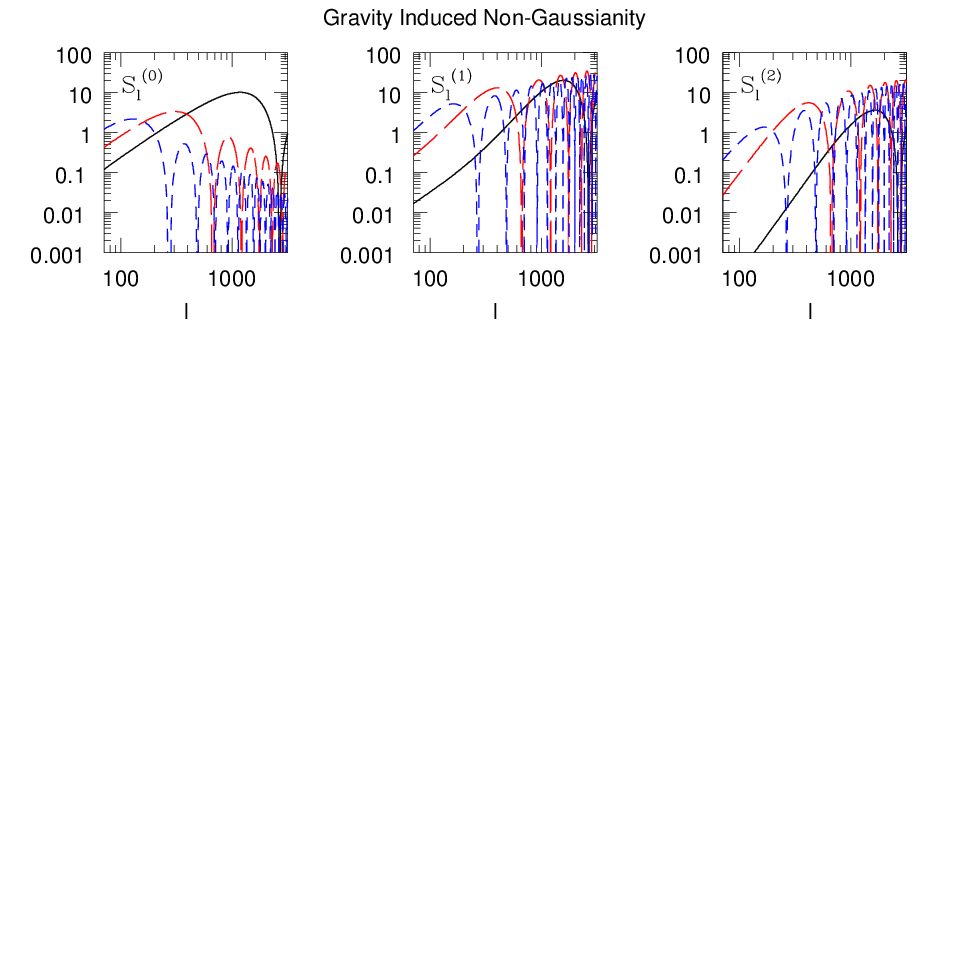
Results from the Halo Model analysis are plotted for the skew-spectra $S_{l}^{(0)}$ (left panel), $S_{l}^{(1)}$ (middle panel) and $S_{l}^{(2)}$ (right panel). The source redshift is fixed at unity. The underlying background cosmology is that of WMAP7. No smoothing window was assumed. A sharp cutoff at $l_{max}=2000$ was used for this calculations. As mentioned, halos in the mass range of $10^{3}M_{☉}-10^{16}M_{☉}$ were included in this calculation. The halo model expression for the bispectrum is defined in Eq.(38) - Eq.(40).

5.3 Perturbative calculations in the quasi-linear regime and their extensions

In the weakly non-linear regime ( $\delta\leq 1$ ), the description of gravitational clustering can be described by perturbation theory Bernardeau et al (2002). However, the perturbative treatment breaks down when density contrast at a given length scale becomes nonlinear ( $\delta\geq 1$ ) which significantly increases the growth of clustering. Perturbative studies of gravitational clustering have attracted a lot of attention. Starting with Peebles (1980), there have been many attempts to reproduce the clustering of a self-gravitating fluid in a cosmological setting is typically tackled by brute force using N-body simulations Bernardeau et al (2002). Expanding the density contrast in a Fourier series, and assuming the density contrast is less than unity, for the pertubative series to be convergent, we get

\delta({\bf k})=\delta^{(1)}({\bf k})+\delta^{(2)}({\bf k})+\delta^{(3)}({\bf k})+\dots;\quad\delta^{(2)}(k)=\int{d^{3}k_{1}\over 2\pi}\int{d^{3}k_{2}\over 2\pi}\delta_{D}({\bf k_{1}+k_{2}-k})F_{2}(k_{1},k_{2})\delta^{(1)}({\bf k}_{1})\delta^{(1)}({\bf k}_{2}).

(42)

The linearized solution for the density field is $\delta^{(1)}({\bf k})$ ; higher-order terms yield corrections to this linear solution. Using a fluid approach known to be valid at large scales (and before shell crossing) one can write the second order correction to the linearized density field using the kernel $F_{2}({\bf k_{1}},{\bf k_{2}})$ . Newtonian gravity coupled to the Euler and continuity equation employed to solve a system of non-linear coupled integro-differential equation reproduces the kernels $F_{2}(k_{1},k_{2})$ $F_{3}(k_{1},k_{2},k_{3})$ when solved perturbatively order by order. The expression for the matter bispectrum can be written in terms of an effective fitting formula that can interpolate between quasilinear regime and the highly nonlinear regime:

	$\displaystyle B_{\delta}({\bf k}_{1},{\bf k}_{2},{\bf k}_{3})=2F_{2}({\bf k_{1}},{\bf k_{2}})P_{lin}^{\delta}({\bf k}_{1})P_{lin}^{\delta}({\bf k}_{2})+{\rm cyc.perm.};{}$
	$\displaystyle F_{2}({\bf k_{1}},{\bf k_{2}})={5\over 7}a(n_{e},k)a(n_{e},k)+\left({{\bf k}_{1}\cdot{\bf k}_{2}\over 2k_{2}^{2}}+{{\bf k}_{1}\cdot{\bf k}_{2}\over 2k_{1}^{2}}\right)b(n_{e},k)b(n_{e},k)+{2\over 7}\left({{\bf k}_{1}\cdot{\bf k}_{2}\over k_{1}k_{2}}\right)^{2}c(n_{e},k)c(n_{e},k)$		(43)

The coefficients $a({n_{e}},k),b({n_{e}},k)$ and $c({n_{e}},k)$ are defined as follows:

a(n_{e},k)={1+\sigma_{8}^{-0.2}(z)\sqrt{(q/4)^{n_{e}+3.5}}\over 1+(q/4)^{n_{e}+3.5}};\quad b(n_{e},k)={1+0.4(n_{e}+3)q^{n_{e}+3}\over 1+q^{n_{eff}+3}};\quad c(n_{e},k)={(2q)^{n_{e}+3}\over 1+(2q)^{n_{e}+3.5}}\left\{{1+\left(4.5\over 1.5+(n_{e}+3)^{4}\right)}\right\}

(44)

Here $n_{e}$ is the effective spectral slope associated with the linear power spectra $n_{e}=d\ln P_{{}_{\rm{lin}}}/d\ln k$ , q is the ratio of a given length scale to the non-linear length scale $q=k/k_{nl}$ , where ${k^{3}/2\pi^{2}}D^{2}(z)P{{}_{\rm{lin}}}(k_{nl})=1$ and $Q_{3}(n_{e})={(4-2^{n_{e}})/(1+2^{n_{e}})}$ . Similarly $\sigma_{8}(z)=D(z)\sigma_{8}$ . At length scales where $q\ll 1$ which means the relevant length scales are well within the quasilinear regime $a=b=c=1$ and we recover the tree-level perturbative results. In the regime when $q\gg 1$ and the length scales we are considering are well within the nonlinear scale we recover $a=\sigma_{r}^{-0.2}(z)\sqrt{0.7Q_{3}(n_{e})}$ with $b=c=0.$ In this limit the bispectrum becomes independent of configuration and we recover the hierarchical form of bispectrum discussed before. However is there are weak violations of hierarchical ansatz in the highly nonlinear regime is still not clear and can only be determined higher resolution N-body simulations when they are available. Similar fitting functions for dark energy dominated universe calibrated against simulations are also available and at least in the quasilinear regime most of the difference comes from the linear growth factor (Ma et al., 1999). The analytical modeling of the matter bispectrum presented here is equivalent to the so-called Halo Model predictions presented above.

We have used this model to construct the analytical predictions for various skewness parameters and the corresponding skew-spectra. The results are plotted in Figures 3, 4, 6 and 7. In Figure 3 we have plotted the three skewness parameters $S^{(0)},S^{(1)}$ and $S^{(2)}$ as a function of the smoothing angular scales $\theta_{s}$ as defined in Eq.(2). In Figure-4 we change the source redshift to compare predictions. In total we compare three different redshifts $z_{s}=0.5,1.0$ and $z_{s}=1.5$ respectively. We use top hat filters with different angular smoothing scales. The skew-spectra, defined in Eq.(23), are integrated measures and their value at a specific harmonic depends on modelling of the bispectrum for the entire range of harmonics being considered. The skew spectra are plotted as functions of harmonic $l$ in Figure 6 and Figure 7 respectively. In Figure 6 we consider the redshift $z_{s}=1.0$ and in Figure 7 results for two different redshifts, $z_{s}=0.5$ and $z_{s}=1.5$ , are compared for a given angular smoothing. The oscillatory behaviour seen in these plots is due to our choice of fiter function i.e. top hat window.

5.4 Primordial non-Gaussianity: bispectrum

A recent (controversial) claim of a detection of non-Gaussianity (Yadav & Wandelt, 2008) in the Wilkinson Microwave Anisotropy Probe 5-year (WMAP5) sky maps, has boosted interest in cosmological non-Gaussianity. Much of the interest in primordial non-Gaussianity has focussed on a phenomenological ‘local $f_{NL}$ ’ parametrization in terms of the perturbative non-linear coupling in the primordial curvature perturbation (Verde et al., 2007):

\Phi(x)=\Phi_{L}(x)+f_{NL}(\Phi^{2}_{L}(x)-\langle\Phi^{2}_{L}(x)\rangle),

(45)

where $\Phi_{L}(x)$ denotes the linear Gaussian part of the Bardeen curvature and $f_{NL}$ is the non-linear coupling parameter. A number of models have non-Gaussianity which can be approximated by this form. The leading order non-Gaussianity present in this model is at the level of the bispectrum, or in configuration space at the three-point level. Many studies involving primordial non-Gaussianity have used the bispectrum, motivated by the fact that it contains all the information about $f_{NL}$ (Babich, 2005). This model has been extensively studied (Komatsu, Spergel & Wandelt, 2005; Creminelli, 2003; Creminelli et al., 2006; Medeiros & Contaldi, 2006; Cabella et al., 2006; Smith, Senatore & Zaldarriaga, 2009), with most of these measurements providing convolved estimates of the bispectrum. It is interesting to note here in the context of bispectrum estimation from CMB sky, optimized 3-point estimators were introduced by Heavens (1998), and have been successively developed (Komatsu, Spergel & Wandelt, 2005; Creminelli et al., 2006; Creminelli, Senatore, & Zaldarriaga, 2007; Smith, Zahn & Dore, 2000; Smith & Zaldarriaga, 2006) to the point where an estimator for $f_{NL}$ which saturates the Cramer-Rao bound exists for partial sky coverage and inhomogeneous noise (Smith, Senatore & Zaldarriaga, 2009). Approximate forms also exist for equilateral non-Gaussianity, which may arise in models with non-minimal Lagrangian with higher-derivative terms (Chen, Huang & Kachru, 2006; Chen, Easther & Lim, 2007). In these models, the largest signal comes from spherical harmonic modes with $\ell_{1}\simeq\ell_{2}\simeq\ell_{3}$ , whereas for the local model, the signal is highest when one $\ell$ is much smaller than the other two – the so-called squeezed configuration.

In the Fourier space the primordial bispectrum of local type defined in Eq.(45) takes the following form:

B_{\delta}^{loc}({\bf k}_{1}{\bf k}_{1},{\bf k}_{3})=2f_{NL}^{\rm loc}\left[P^{\Phi}_{\rm lin}(k_{1})P^{\Phi}_{\rm lin}(k_{2})+{\rm cyc.perm.}\right].

(46)

The primordial potential power spectrum in standard inflationary models takes a power law form $P^{\Phi}(k)\propto k^{n-4}$ . In the linear regime, the primordial bispectrum for the density field $B_{\delta}^{\rm prim}$ in case of local model evolves according to the following expression (see Hikage et al. (2006) for a detailed derivation and discussion):

	$\displaystyle B_{\delta}^{\rm loc}({\bf k}_{1}{\bf k}_{1},{\bf k}_{3};z)={2f_{NL}^{\rm loc}\over D(z)}\left[{{\cal M}({k_{3}})\over{\cal M}({k_{1}}){\cal M}({k_{2}})}P^{\delta}_{\rm lin}(k_{1},z)P^{\delta}_{\rm lin}(k_{2},z)+{\rm cyc.perm.}\right];\quad$		(47)
	$\displaystyle\delta({\bf k},z)=D(z){\cal M}(k)\Phi({\bf k},z);\quad{\cal M}(k)\equiv-{2\over 3H_{0}^{2}\Omega_{m}}k^{2}T(k).$		(48)

Here $D(z)$ is the linear growth factor normalised such that $D(z)\rightarrow{1/(1+z)}$ and $T(k)$ is the transfer function given by an approximate expression found in BBKS (1986). According to standard inflationary predictions $P^{\Phi}(k)\propto k^{n-4}$ and the linear power spectra for the density is given by $P^{\delta}_{lin}(k,z)=D^{2}(z){\cal M}(k)^{2}P^{\Phi}(k)$ . The primordial bispectrum for the density can similarly be expressed in terms of that of the primordial potential perturbations $B_{\delta}^{prim}(k_{1},k_{2},k_{3},z)=D^{3}(z){\cal M}(k_{1}){\cal M}(k_{2}){\cal M}(k_{3})B_{\Phi}^{prim}(k_{1},k_{2},k_{3})$ . The primordial potential bispectrum for the equilateral type can be expressed as (Creminelli et al., 2006):

B^{equi}_{\phi}=6f^{equi}_{NL}\left[-(P_{\Phi}(k_{1})P_{\Phi}(k_{2})+cyc.perm.)-2(P_{\Phi}(k_{1})P_{\Phi}(k_{2})P_{\Phi}(k_{3}))^{2/3}+(P^{1/3}_{\Phi}(k_{1})P^{2/3}_{\Phi}(k_{2})P_{\Phi}(k_{2})+cyc.perm.)\right]

(49)

The primordial density bispectrum for the equilateral case $B_{\delta}^{equi}$ can be expressed, following the same procedure that we followed for the local type, as:

$\displaystyle B_{\delta}^{equi}({\bf k}_{1}{\bf k}_{1},{\bf k}_{3};z)=$	$\displaystyle{6f_{NL}^{equi}\over D(z)}\Big[-\left({{\cal M}{(k_{3})}\over{\cal M}{(k_{1})}{\cal M}{(k_{2})}}P^{\delta}_{lin}(k_{1},z)P^{\delta}_{lin}(k_{2},z)+cyc.perm.\right){}$	(50)
	$\displaystyle-2\left({{\cal M}{(k_{1})}{\cal M}{(k_{2})}{\cal M}{(k_{3})}}\right)^{-1/3}\{{P^{\delta}_{lin}(k_{1},z)P^{\delta}_{lin}(k_{2},z)P^{\delta}_{lin}(k_{3},z)}\}^{2/3}{}$
	$\displaystyle+\left({{\cal M}{(k_{1})}^{1/3}\over{\cal M}{(k_{2})}^{1/3}{\cal M}{(k_{3})}}\{{{P^{\delta}_{lin}(k_{1},z)P^{\delta}_{lin}(k_{2},z)^{2}P^{\delta}_{lin}(k_{3},z)^{3}}\}^{1/3}+cyc.perm.}\right)\Big].$

However in contrast to the local model , in the equilateral model the functional form of the expressions do not have any connection to fundamental physics but are just fits where the exact expressions are more complicated. The folded or flattened model that is maximized for $k_{2}\approx k_{3}\approx k_{1}/2$ is well approximated by the following form:

B^{fold}_{\phi}=6f^{fold}_{NL}\left[(P_{\Phi}(k_{1})P_{\Phi}(k_{2})+cyc.perm.)+3(P_{\Phi}(k_{1})P_{\Phi}(k_{2})P_{\Phi}(k_{3}))^{2/3}-(P^{1/3}_{\Phi}(k_{1})P^{2/3}_{\Phi}(k_{2})P_{\Phi}(k_{2})+cyc.perm.)\right]

(51)

In terms of the density perturbations, we get the following expression:

$\displaystyle B_{\delta}^{fol}({\bf k}_{1}{\bf k}_{1},{\bf k}_{3};z)=$	$\displaystyle{6f_{NL}^{fol}\over D(z)}\Big[\left({{\cal M}{(k_{3})}\over{\cal M}{(k_{1})}{\cal M}{(k_{2})}}P^{\delta}_{lin}(k_{1},z)P^{\delta}_{lin}(k_{2},z)+cyc.perm.\right){}$	(52)
	$\displaystyle 3\left({{\cal M}{(k_{1})}{\cal M}{(k_{2})}{\cal M}{(k_{3})}}\right)^{-1/3}\{{P^{\delta}_{lin}(k_{1},z)P^{\delta}_{lin}(k_{2},z)P^{\delta}_{lin}(k_{3},z)}\}^{2/3}{}$
	$\displaystyle-\left({{\cal M}{(k_{1})}^{1/3}\over{\cal M}{(k_{2})}^{1/3}{\cal M}{(k_{3})}}\{{{P^{\delta}_{lin}(k_{1},z)P^{\delta}_{lin}(k_{2},z)^{2}P^{\delta}_{lin}(k_{3},z)^{3}}\}^{1/3}+cyc.perm.}\right)\Big].$

The folded or flattened form of bispectrum appears in canonical single field models where the initial Bunch-Davies vacuum is modified.

The evolution of the primordial bispectrum is different to that generated by gravitational evolution. The angular dependence for the gravitationally-induced bispectrum is also different. On large angular scales, which will be probed by future weak lensing surveys, gravitational instability may not have erased the memory of primordial non-Gaussianity, which can provide supplementary information to results obtained from CMB observations.

6 Estimators and their scatter

As noted above, the estimators for the skew-spectra can be most easily computed by cross-correlating maps in the harmonic domain. These maps are constructed in real space by applying various derivative operators. The recovered skew-spectra will depend on the mask, if one is present, because a mask typically introduces mode-mode coupling. The approach we adopt here to reconstruct the unbiased power spectra in such a case is the Pseudo- ${\cal C}_{l}$ method (Hivon et al., 2002). This approach depends on expressing the observed power spectra ${\cal C}_{l}$ in the presence of mask as a linear combination of unbiased all-sky power spectra.

The three different generalized skew spectra that we have introduced here can be thought as cross-spectra of relevant fields. We denote these generic fields by $A$ and $B$ and will denote the generic skew-spectra as $S_{l}^{[A,B]}$ . The skew-spectra recovered in the presence of masks will be represented as $\tilde{S}_{l}^{[A,B]}$ and the unbiased estimator will be denoted $\hat{S}_{l}^{[A,B]}$ . The skew-spectra recovered in the presence of mask $\tilde{S}_{l}^{[A,B]}$ will be biased. However to construct an unbiased estimator $\hat{S}_{l}^{[A,B]}$ for the skew-spectra the following procedure is sufficient. The derivation follows the same arguments as detailed in Munshi, Smidt & Cooray (2010) and will not be reproduced here.

\tilde{S}_{l}^{[A,B]}={1\over 2l+1}\sum_{m}\tilde{A}_{lm}\tilde{B}^{*}_{lm};\quad\tilde{S}_{l}^{[A,B]}=\sum_{l^{\prime}}M_{ll^{\prime}}S_{l}^{[A,B]};\quad M_{ll^{\prime}}={1\over 2l+1}\sum_{l^{\prime}l^{\prime\prime}}I^{2}_{ll^{\prime}l^{\prime\prime}}|w_{l^{\prime\prime}}|^{2};\quad\left\{A,B\right\}\in\left\{\kappa,\kappa^{2},(\nabla\kappa\cdot\nabla\kappa),\nabla^{2}\kappa\right\}.\\

(53)

The mode-mode coupling matrix $M$ is constructed from the power spectra of the mask $w_{l^{\prime\prime}}$ and used for estimation of unbiased skew-spectra $\hat{S}_{l^{\prime}}^{A,B}$ . Typically the mask consists of bright stars and saturated spikes where no lensing measurements can be performed. The results that we present here are generic. The estimator thus constructed is an unbiased estimator. The computation of the scatter covariance of the estimates can be computed using analytical methods, thereby avoiding the need of expensive Monte-Carlo simulations. The scatter or covariance of the unbiased estimates $\langle\delta\hat{S}_{l}^{A,B}\delta\hat{S}_{l^{\prime}}^{A,B}\rangle$ is related to that of the direct estimates $\langle\delta\tilde{S}_{l}^{A,B}\delta\tilde{S}_{l^{\prime}}^{A,B}\rangle$ from the masked sky by a similarity transformation. The transformation is given by the same mode coupling matrix $M$ :

\hat{S}_{l}^{[A,B]}=\sum_{l^{\prime}}[M^{-1}]_{ll^{\prime}}\tilde{S}_{l^{\prime}}^{[A,B]};\quad\langle\delta\hat{S}_{l}^{[A,B]}\delta\hat{S}_{l^{\prime}}^{[A,B]}\rangle=\sum_{LL^{\prime}}M^{-1}_{lL}\langle\delta\tilde{S}_{L}^{[A,B]}\delta\tilde{S}_{L^{\prime}}^{[A.B]}\rangle M^{-1}_{L^{\prime}l^{\prime}};\quad\langle\hat{S}_{l}^{[A,B]}\rangle=S_{l}^{[A,B]}.{}\\

The power-spectra associated with the MFs are linear combinations of the skew-spectra (see Eq.(3)). In our approach the power spectra associated with the MFs are secondary and can be constructed using the skew-spectra that are estimated directly from the data.

No construction of an estimator is complete without an estimate of its variance. The variance or the scatter in certain situations can be computed using Monte-Carlo (MC) simulations which are computationally expensive. In our approach, it is possible to compute the covariance of our estimates of various $S_{l}$ s, i.e. ${\langle\delta S_{l}\delta S_{l^{\prime}}\rangle}$ under the same simplifying assumptions that higher-order correlation functions can be approximated as Gaussian. This allows us to express the error covariance in terms of the relevant power spectra. The generic expression can be written

[\hat{V}_{k}^{(2)}]_{l}=\sum_{l^{\prime}}[M^{-1}]_{ll^{\prime}}[\tilde{V}_{k}^{(2)}]_{l};\quad\quad\langle\delta\hat{V}_{k}^{(2)}\delta\hat{V}_{k^{\prime}}^{(2)}\rangle=\sum_{LL^{\prime}}M^{-1}_{lL}\langle\delta[\tilde{V}_{k}^{(2)}]_{l}\delta[\tilde{V}_{k^{\prime}}^{(2)}]_{l^{\prime}}\rangle M^{-1}_{L^{\prime}l^{\prime}}

(54)

We would like to point out here that, in case of limited sky coverage, it may not be possible to estimate the skew-spectra mode by mode as the mode coupling matrix may become singular and a broad binning of the specra may be required.

\displaystyle\langle[\delta S_{l}^{[X,Y]}]\delta S_{l^{\prime}}^{[X,Y]}]\rangle=f^{-1}_{sky}{2\over 2l+1}\left[{\cal C}_{l}^{[X,X]}{\cal C}_{l^{\prime}}^{[Y,Y]}+[S_{l}^{[X,Y]}]^{2}\right]\delta_{ll^{\prime}};\quad\quad\{X,Y\}\in\{\kappa,\kappa^{2},\nabla\kappa({\hat{\Omega}})\cdot\nabla\kappa({\hat{\Omega}}),\nabla^{2}\kappa({\hat{\Omega}})\}.

(55)

Here the fraction of sky covered by the survey is denoted by $f_{\rm sky}$ . The expressions for the skew-spectra are quoted in $S_{l}^{(\kappa^{2},\kappa)}$ , $S_{l}^{(\kappa^{2},\nabla^{2}\kappa)}$ and $S_{l}^{(\nabla\kappa\cdot\nabla\kappa,\nabla^{2}\kappa)}$ are given in Eq.(23). The expressions for covariance also depend on a set of power spectra i.e. $S_{l}^{(\kappa^{2},\kappa^{2})}$ , $S_{l}^{(\nabla^{2}\kappa,\nabla^{2}\kappa)}$ , $S_{l}^{(\nabla\kappa\cdot\nabla\kappa,\nabla^{2}\kappa)}$ and $S_{l}^{\kappa,\kappa}$ . These are given by the following expression:

	$\displaystyle{\cal C}_{l}^{\nabla\cdot\nabla,\nabla\cdot\nabla}=\sum_{l^{\prime}l^{\prime\prime}}({\cal C}_{l^{\prime}}+N_{l^{\prime}})({\cal C}_{l^{\prime\prime}}+N_{l^{\prime\prime}})[l_{1}(l_{1}+1)+l_{2}(l_{2}+1)-l(l+1)]^{2}I^{2}_{ll^{\prime}l^{\prime\prime}}W_{l^{\prime}}W_{l^{\prime\prime}};$		(56)
	$\displaystyle{\cal C}_{l}^{[\kappa^{2},\kappa^{2}]}=\sum_{l^{\prime}l^{\prime\prime}}({\cal C}_{l^{\prime}}+N_{l^{\prime}})({\cal C}_{l^{\prime\prime}}+N_{l^{\prime\prime}})I^{2}_{ll^{\prime}l^{\prime\prime}}W_{l^{\prime}}W_{l^{\prime\prime}};\quad{\cal C}_{l}^{[\nabla^{2}\kappa,\nabla^{2}\kappa]}=l^{2}(l+1)^{2}({\cal C}_{l}+N_{l})W_{l}$		(57)

Here ${\cal C}_{l}$ is the ordinary ”theoretical” convergence power spectrum defined in Eq.(14) that includes noise i.e. ${\cal C}_{l}W_{l}$ is replaced with ${\cal C}_{l}W_{l}+N_{l}$ with $N_{l}=4\pi\sigma_{i}^{2}/N_{gal}$ . Here $\sigma_{i}$ is the intrinsic ellipticity distribution of galaxies and $N_{gal}$ is the number of galaxies per arc-minute square. Using these equations it is possible to compute the scatter in various skew-spectra. These results can also be extended to take into account the cross-correlation among various skew-spectra extracted from the same data. Using a less compact notation we can write

	$\displaystyle\langle\delta S_{l}^{[\kappa^{2},\kappa]}\delta S_{l}^{[\kappa^{2},\kappa]}\rangle=f^{-1}_{\rm sky}{1\over 2l+1}\left[{\cal C}_{l}^{[\kappa^{2},\kappa^{2}]}{\cal C}_{l}^{[\kappa,\kappa]}+[S_{l}^{[\kappa^{2},\kappa]}]^{2}\right]$		(58)
	$\displaystyle\langle\delta S_{l}^{[\kappa^{2},\nabla^{2}\kappa]}\delta S_{l}^{[\kappa^{2},\nabla^{2}\kappa]}\rangle=f^{-1}_{\rm sky}{1\over 2l+1}\left[{\cal C}_{l}^{[\kappa^{2},\kappa^{2}]}{\cal C}_{l}^{[\nabla\cdot\nabla,\nabla\cdot\nabla]}+[S_{l}^{[\kappa^{2},\nabla^{2}\kappa]}]^{2}\right]$		(59)
	$\displaystyle\langle\delta S_{l}^{[\nabla\kappa\cdot\nabla\kappa,\nabla^{2}\kappa]}\delta S_{l}^{[\nabla\kappa\cdot\nabla\kappa,\nabla^{2}\kappa]}\rangle=f^{-1}_{\rm sky}{1\over 2l+1}\left[{\cal C}_{l}^{[\nabla^{2}\kappa,\nabla^{2}\kappa]}{\cal C}_{l}^{[\nabla\cdot\nabla,\nabla\cdot\nabla]}+[S_{l}^{[\nabla\kappa\cdot\nabla\kappa,\nabla^{2}\kappa]}]^{2}\right].$		(60)

The cumulative signal to noise upto a given $l_{max}$ using these expression for estimators $S^{(0)}$ can now be expressed as:

\displaystyle\left[\left({S\over N}\right)^{0}_{lmax}\right]^{2}=f_{sky}\sum_{l}^{l_{max}}(2l+1)\left\{(S_{l}^{[\kappa^{2},\kappa]})^{2}\over\left[{\cal C}_{l}^{[\kappa^{2},\kappa^{2}]}{\cal C}_{l}^{[\kappa,\kappa]}+(S_{l}^{[\kappa^{2},\kappa]})^{2}\right]\right\}

(61)

The signal-to-noise for the other two estimators $S^{(1)}$ and $S^{(2)}$ can be defined likewise. The different skew-spectra that we have studied here are not completely independent. Their covariance can be analysed using the same procedure, allowing their joint estimation from a single data set.

	$\displaystyle\langle\delta S_{l}^{[\kappa^{2},\kappa]}\delta S_{l}^{[\kappa^{2},\nabla^{2}\kappa]}\rangle=f^{-1}_{\rm sky}{1\over 2l+1}\left[{\cal C}_{l}^{[\kappa^{2},\kappa^{2}]}{\cal C}_{l}^{[\kappa,\nabla^{2}\kappa]}+S_{l}^{[\kappa^{2},\nabla^{2}\kappa]}S_{l}^{[\kappa,\kappa^{2}]}\right]$		(62)
	$\displaystyle\langle\delta S_{l}^{[\kappa^{2},\kappa]}\delta S_{l}^{[\nabla\kappa\cdot\nabla\kappa,\nabla^{2}\kappa]}\rangle=f^{-1}_{\rm sky}{1\over 2l+1}\left[S_{l}^{[\kappa^{2},\nabla^{2}\kappa]}{\cal C}_{l}^{[\kappa,\nabla\kappa\cdot\nabla\kappa]}+{\cal C}_{l}^{(\kappa^{2},\nabla\kappa\cdot\nabla\kappa)}{\cal C}_{l}^{(\kappa,\nabla^{2}\kappa)}\right]$		(63)
	$\displaystyle\langle\delta S_{l}^{[\kappa^{2},\nabla^{2}\kappa]}\delta S_{l}^{[\nabla\kappa\cdot\nabla\kappa,\nabla^{2}\kappa]}\rangle=f^{-1}_{\rm sky}{1\over 2l+1}\left[{\cal C}_{l}^{(\kappa^{2},\nabla\kappa\cdot\nabla\kappa)}{\cal C}_{l}^{(\nabla^{2}\kappa,\nabla^{2}\kappa)}+S_{l}^{[\kappa^{2},\nabla^{2}\kappa]}S_{l}^{[\nabla^{2}\kappa,\nabla\kappa\cdot\nabla\kappa]}\right]$		(64)

The above results can be generalized to compute the cross-covariance of $S_{l}$ from different sources of bispectrum. The following quantities are required to compute the necessary cross-covariances.

	$\displaystyle{\cal C}_{l}^{[\kappa,\nabla^{2}\kappa]}=-l(l+1){\cal C}_{l};\quad{\cal C}_{l}^{[\kappa^{2},\nabla\kappa\cdot\nabla\kappa]}=\sum_{l^{\prime}l^{\prime\prime}}({\cal C}_{l^{\prime}}W_{l^{\prime}}+N_{l})({\cal C}_{l^{\prime\prime}}W_{l^{\prime\prime}}+N_{l^{\prime\prime}})I^{2}_{ll^{\prime}l^{\prime\prime}}[l^{\prime}(l^{\prime}+1)+l^{\prime\prime}(l^{\prime\prime}+1)-l(l+1)];\;$		(65)
	$\displaystyle{\cal C}_{l}^{[\kappa,\nabla\kappa\cdot\nabla\kappa]}=-\sum_{l^{\prime}l^{\prime\prime}}[l^{\prime}(l^{\prime}+1)+l^{\prime\prime}(l^{\prime\prime}+1)-l(l+1)]{\cal B}_{ll^{\prime}l^{\prime\prime}}J_{ll^{\prime}l^{\prime\prime}}W_{l^{\prime}}W_{l^{\prime\prime}}$		(66)

We have discussed the lowest-order departure from Gaussianity in MFs using a third order statistic, namely the bispectrum. The next-to-leading descriptions are characterized by the trispectrum which is a fourth order statistics. It is possible to estend the definition of skew-spectra to the case of kurt-spectra or the power spectrum associated with tri-spectra. The power spectra associated with the Minkowski Functionals can be defined completely up to fourth order using the skew- and the kurt-spectra. However, the corrections to leading order statistics from kurt-spectra are sub-dominant and leading order terms are consequently sufficient to study the departure from Gaussianity. In any case it is nevertheless straightforward to implement an estimator which which will estimate the power-spectrum associated with the MFs from noisy data by including both third order and fourth order statistics; this issue has been dealt with in detail in (Munshi, Smidt & Cooray, 2010) in the context of CMB sky. The same results will also be applicable for weak lensing surveys.

In addition to the three genralised skew-spectra that define the MFs at lowest order in non-Gaussianity, it is indeed possible to construct additional skew-spectra that work with different set of weights. In principle arbitrary number of such skew-specta can be constrcuted though they will not have direct links with the morphological properties that we have focussed on, in this paper they can still be used as a source of independent information on the bispectrum and can be used in principle to separate sources of non-Gaussianity, whether primordial or gravity induced.

7 Next to leading order corrections to the Minkowski Functionals from the trispectrum

The skew-spectra $S^{(i)}_{l}$ and the related skewness parameters $S^{(i)}$ completely specify the MFs at leading order. The next-to-leading order corrections are determined by a set of four kurtosis parameters $K^{(i)}$ . These generalised kurtosis parameters are constructed from the trispectrum using varying weights to sample different modes. This method is very similar to construction of the generalised skew-spectra and their associated skewness parameters from the bispectrum described in previous sections. The kurt-spectra are constructed by cross-correlating maps that are constructed from original maps and combinations of maps constructed from the original map e.g. $\nabla\Phi({\hat{\Omega}})$ and $\nabla^{2}\Phi({\hat{\Omega}})$ . The four kurtosis parameters are natural generalizations of the ordinary kurtosis $K^{(0)}$ and can be most easily be estimated in real space. The normalization of these kurtosis parameters are determined by suitable combinations of powers of parameters $\sigma_{0}$ and $\sigma_{1}$ (Matsubara, 2010).

	$\displaystyle K^{(0)}\equiv{1\over\sigma_{0}^{6}}K^{(\kappa^{4})}={\langle\kappa^{4}({\hat{\Omega}})\rangle_{c}\over\sigma_{0}^{6}};\quad K^{(1)}\equiv{1\over\sigma_{0}^{4}\sigma_{1}^{2}}K^{(\kappa^{3}\nabla^{2}\kappa)}={\langle\kappa^{3}({\hat{\Omega}})\nabla^{2}\kappa({\hat{\Omega}})\rangle_{c}\over\sigma_{0}^{4}\sigma_{1}^{2}};\quad$		(67)
	$\displaystyle K^{(2)}\equiv K^{(2a)}+K^{(2b)}\equiv{1\over\sigma_{0}^{2}\sigma_{1}^{4}}K^{(\kappa\|\nabla\kappa\|^{2}\nabla^{2}\kappa)}+{1\over\sigma_{0}^{2}\sigma_{1}^{4}}K^{(\|\nabla\kappa\|^{4})}={}{\langle\kappa\|(\nabla\kappa({\hat{\Omega}}))\|^{2}(\nabla^{2}\kappa({\hat{\Omega}}))\rangle_{c}\over\sigma_{0}^{2}\sigma_{1}^{4}}+{}{\langle\|(\nabla\kappa)\|^{4}\rangle_{c}\over\sigma_{0}^{2}\sigma_{1}^{4}};$		(68)
	$\displaystyle K^{(3)}\equiv{1\over 2\sigma_{0}^{2}\sigma_{1}^{4}}K^{(\|\nabla\kappa\|^{4})}={\langle\|\nabla\kappa({\hat{\Omega}})\|^{4}\rangle_{c}\over 2\sigma_{0}^{2}\sigma_{1}^{4}};\quad{\rm where}\quad\|\nabla\kappa({\hat{\Omega}})\|^{2}=\nabla\kappa({\hat{\Omega}})\cdot\nabla\kappa({\hat{\Omega}}).$		(69)

Unlike the skewness parameters the kurtosis parameters get contributions also from Gaussian (unconnected) components. The subscript $c$ above however refers to the non-Gaussian or the connected part of the contribution which is directly liked to the trispectrum.

The correction to the Minkowski Functionals $\delta V^{(i)}(\nu)$ as defined in Eq.(3) from the next to leading order terms consists of both the Kurtosis parameters $K^{(i)}$ as well as the product of two skewness parameters $S^{(i)}$ (Matsubara, 2010):

	$\displaystyle\delta V_{0}^{(4)}(\nu)={[S^{(0)}]^{2}\over 72}H_{5}(\nu)+{K^{(0)}\over 24}H_{3}(\nu);\quad$		(70)
	$\displaystyle\delta V_{1}^{(4)}(\nu)={[S^{(0)}]^{2}\over 72}H_{6}(\nu)+\left[{K^{(0)}-S^{(0)}S^{(1)}\over 24}\right]H_{4}(\nu)-{1\over 12}\left[K_{1}+{3\over 8}[S^{(1)}]^{2}\right]H_{2}(\nu)-{1\over 8}K^{(3)}{}$
	$\displaystyle\delta V_{2}^{(4)}(\nu)={[S^{(0)}]^{2}\over 72}H_{7}(\nu)+\left[{K^{(0)}-S^{(0)}S^{(1)}\over 24}\right]H_{5}(\nu)-{1\over 6}\left[K^{(1)}+{1\over 2}S^{(0)}S^{(2)}\right]H_{3}(\nu)-{1\over 2}\left[K^{(2)}+{1\over 2}S^{(1)}S^{(2)}\right]H_{1}(\nu).$		(71)

The analytical modelling of four-point correlation functions is most naturally done in the harmonic domain. They are described by the angular trispectrum ${\cal T}^{l_{1}l_{2}}_{l_{3}l_{4}}(L)$ which is defined through the relation $\langle\kappa_{l_{1}m_{1}}\kappa_{l_{2}m_{2}}\kappa_{l_{3}m_{3}}\kappa_{l_{4}m_{4}}\rangle_{c}=\sum_{L}I_{l_{1}l_{2}L}I_{l_{3}l_{4}L}{\cal T}^{l_{1}l_{2}}_{l_{3}l_{4}}(L)$ . The trispectrum ${\cal T}^{l_{1}l_{2}}_{l_{3}l_{4}}(l)$ is expressed in terms of the reduced trispectrum $P^{l_{1}l_{2}}_{l_{3}l_{4}}(l)$ . Following expression was introduced by (Hu, 2000; Hu, 2001; Hu & Okamoto, 2002) and encodes all possible inherent symmetries.

{\cal T}^{l_{1}l_{2}}_{l_{3}l_{4}}(l)=P^{l_{1}l_{2}}_{l_{3}l_{4}}(l)+(2l+1)\left[\sum_{l^{\prime}}(-1)^{l_{2}+l_{3}}\left\{\begin{array}[]{ c c c }l_{1}&l_{2}&l\\ l_{4}&l_{3}&l^{\prime}\end{array}\right\}P^{l_{1}l_{3}}_{l_{2}l_{4}}(l^{\prime})+\sum_{l^{\prime}}(-1)^{L+L^{\prime}}\left\{\begin{array}[]{ c c c }l_{1}&l_{2}&l\\ l_{3}&l_{4}&l^{\prime}\end{array}\right\}P^{l_{1}l_{4}}_{l_{3}l_{2}}(l^{\prime})\right].

(72)

The matrices in curly brackets represent $6j$ symbols which are defined using $3j$ symbols; see Edmonds (1968) for more detailed discussions. The entities $P^{l_{1}l_{2}}_{l_{3}l_{4}}(l)$ can be further decomposed in terms of the reduced trispectrum $\tau^{l_{1}l_{2}}_{l_{3}l_{4}}(l)$ . A specific model for the non-Gaussianity - either primordial or gravity-induced - has a specific prescription for the reduced trispectrum which in turn describes the next-to-leading-order corrections to the MFs.

P^{l_{1}l_{2}}_{l_{3}l_{4}}(l)=\tau^{l_{1}l_{2}}_{l_{3}l_{4}}(l)+(-1)^{\Sigma_{U}}\tau^{l_{2}l_{1}}_{l_{3}l_{4}}(l)+(-1)^{\Sigma_{L}}\tau^{l_{1}l_{2}}_{l_{4}l_{3}}(l)+(-1)^{\Sigma_{L}+\Sigma_{U}}\tau^{l_{2}l_{1}}_{l_{4}l_{3}}(l);\quad\Sigma_{L}=l_{1}+l_{2}+l;\quad\Sigma_{U}=l_{3}+l_{4}+l.

(73)

In addition to the original convergence trispectra $[{\cal T}^{(0)}]$ generally used in the literature we can define a set of four trispectra which uses different weights to samples of modes deefined by the quadruplet of harmonic numbers ${l_{i}}$ .

	$\displaystyle[{\cal T}^{(0)}]^{l_{1}l_{2}}_{l_{3}l_{4}}(l)={\cal T}^{l_{1}l_{2}}_{l_{3}l_{4}}(l);\quad[T^{(1)}]^{l_{1}l_{2}}_{l_{3}l_{4}}(l)={1\over 4}\left[{l_{1}(l_{1}+1)+l_{2}(l_{2}+1)+l_{3}(l_{3}+1)+l_{4}(l_{4}+1)}\right]{\cal T}^{l_{1}l_{2}}_{l_{3}l_{4}}(l);$		(74)
	$\displaystyle[{\cal T}^{(2)}]^{l_{1}l_{2}}_{l_{3}l_{4}}(l)={1\over 4}\left[{l(l+1)-(l_{1}(l_{1}+1)+l_{2}(l_{2}+1))(l_{3}(l_{3}+1)+l_{4}(l_{4}+1))}\right]{\cal T}^{l_{1}l_{2}}_{l_{3}l_{4}}(l);$		(75)
	$\displaystyle[{\cal T}^{(3)}]^{l_{1}l_{2}}_{l_{3}l_{4}}(l)={1\over 4}\left[{(l_{1}(l_{1}+1)+l_{2}(l_{2}+1)-l(l+1))(l_{3}(l_{3}+1)+l_{4}(l_{4}+1)-l(l+1))}\right]{\cal T}^{l_{1}l_{2}}_{l_{3}l_{4}}(l).$		(76)

The power spectrum associated with these kurtosis parameters, i.e. the kurt-spectrum, is defined in terms of the trispectrum, extending the previously defined skew-spectra along fairly obvious lines. The estimation of these kurt-spectra would be done by cross-correlating relevant fields used to construct the related kurtosis in real space $K^{(i)}$ :

K^{(i)}=\sum_{l_{i}}\sum_{L}[{\cal T}^{(i)}]^{l_{1}l_{2}}_{l_{3}l_{4}}(L)I_{l_{1}l_{2}L}I_{l_{3}l_{4}L};\quad K^{(i)}_{l}=\sum_{l_{i}}[{\cal T}^{(i)}]^{l_{1}l_{2}}_{l_{3}l_{4}}(l)J_{l_{1}l_{2}l}J_{l_{3}l_{4}l};\quad\sum_{i}(2l+1)K^{(i)}_{l}=K^{(i)}.

(77)

The error and covariance associated with these kurt-spectra can be computed using exactly the same formalism that we described in the context of estimation of skew-spectra. The kurt-spectra being a power spectra will contain more information compared to the kurtosis which is a one-point estimator. Though one may be interested in principle to extract the entire trispectrum, it may be more realistic to use the kurt-spectra because of the likely low signal-to-noise associated with individual harmonic modes.

To compute the kurtosis one needs a resonable model to compute the trispectra for the convergence field. This is typically done using the paraphernalia of the Halo Model we introduced before. The modelling of the gravity-induced trispectrum in the Halo Model follows the same principle as before. It involves contributions from one-, two-, three- and four-halo contributions and the total can be written as:

T_{\delta}(k_{1},k_{2},k_{3},k_{4})=T^{1h}_{\delta}(k_{1},k_{2},k_{3},k_{4})+T^{2h}_{\delta}(k_{1},k_{2},k_{3},k_{4})+T^{3h}_{\delta}(k_{1},k_{2},k_{3},k_{4})+T^{4h}_{\delta}(k_{1},k_{2},k_{3},k_{4})

(78)

The expressions for various contributions are listed below. These can be expressed in terms of $I^{\beta}_{\mu}(k_{1},k_{2},\dots,k_{\mu};z)$ defined above. Notice that two-halo (2h) term has two contributions. In the case of one represented by $T^{2h}_{31}$ there are three points in the first halo and one in the second. Whereas $T^{2h}_{22}$ represents two points in each halo.

	$\displaystyle T^{1h}_{\delta}=I_{4}^{0}(k_{1},k_{2},k_{3},k_{4});$		(79)
	$\displaystyle T^{2h}_{\delta}=T^{31}+T^{22};\qquad T^{2h}_{31}=P^{\delta}_{lin}(k_{1})I^{1}_{3}(k_{2},k_{3},k_{4})I^{1}_{1}(k_{1})+{\rm cyc.perm.};\qquad T^{2h}_{22}=P^{\delta}_{lin}(k_{1}2)I^{1}_{2}(k_{1},k_{2})I^{1}_{2}(k_{3},k_{4})+{\rm cyc.perm.}$		(80)
	$\displaystyle T^{3h}_{\delta}=B^{\delta}_{lin}(k_{1},k_{2},k_{3})I^{1}_{2}(k_{3},k_{4})I^{1}_{1}(k_{1})I^{1}_{1}(k_{2})+P^{\delta}_{lin}(k_{1})P^{\delta}_{lin}(k_{2})I^{2}_{2}(k_{3},k_{4})I^{1}(k_{1})I^{1}_{1}(k_{2})+{\rm cyc.perm.}$		(81)
	$\displaystyle T^{4h}_{\delta}=I^{1}_{1}(k_{1})I^{1}_{1}(k_{2})I^{1}_{1}(k_{3})I^{1}_{1}(k_{4})T^{\delta}_{lin}(k_{1},k_{2},k_{3},k_{4})+I^{2}_{2}(k_{4})I^{1}_{1}(k_{1})I^{1}_{1}(k_{2})I^{1}_{1}(k_{3})+{\rm cyc.perm}$		(82)

Here $P^{\delta}_{lin}$ is the linear power spectrum for the density contrast $\delta$ and $B^{\delta}_{lin}(k_{1},k_{2},k_{3})$ and $T^{\delta}_{lin}(k_{1},k_{2},k_{3},k_{4})$ is the tree level expression for the bispectrum in quasilinear regime. The general expression for $I^{\mu}(k_{1},k_{2},\dots,k_{\mu};z)$ is quoted in the expression Eq.(41). Detailed derivations and discussions of these expressions can be found in e.g. Cooray (2001); Cooray & Seth (2002). Extension of perturbative approaches can also be employed for computation of gravity induced trispectrum. The accuracy of any analytical modeling is more difficult for the higher order multispectra and depends by and large on more inputs from numerical simulations. The projected tripsectrum or the convergence trispectrum ${\cal T}^{l_{1}l_{2}}_{l_{3}l_{4}}(l)$ can be expressed in terms of the underlying mass trispectrum $T^{l_{1}l_{2}}_{l_{3}l_{4}}(l)$ :

{\cal T}^{l_{1}l_{2}}_{l_{3}l_{4}}(l)=I_{l_{1}l_{2}l}I_{l_{3}l_{4}l}\int_{0}^{r_{s}}dr{w^{4}(r,r_{s})\over d^{6}_{A}(r)}T^{\delta}\left({l_{1}\over d_{A}(r)},{l_{2}\over d_{A}(r)},{l_{3}\over d_{A}(r)},{l_{4}\over d_{A}(r)}\right)

(83)

The trispectrum for primordial non-Gaussianity exists in the literature for the local model . The results presented here clearly are generic and can be deployed to analyze arbitrary models. It is worth mentioning here that while modelling of trispectrum is relevant for computation of corrections to the leading order terms they are also important in modelling the scatter in computation of ordinary power spectrum. Hence the errors in $\sigma_{0}$ and $\sigma_{1}$ e.g. will involve the one-point kurtosis parameters $K^{(i)}$ if contributions from non-Gaussianity are taken into account. The correlation functions that represent these kurt-spectra in real space are constructed using derivative operators on the original convergence map and can be useful for surveys with smaller sky coverage.

	$\displaystyle K^{(0)}({\hat{\Omega}}_{1},{\hat{\Omega}}_{2})\equiv\langle\kappa^{2}({\hat{\Omega}}_{1}))\kappa^{2}({\hat{\Omega}}_{2})\rangle_{c};\quad K^{(1)}({\hat{\Omega}}_{1},{\hat{\Omega}}_{2})\equiv\langle\kappa^{2}({\hat{\Omega}}_{1})[\kappa({\hat{\Omega}}_{2})\nabla^{2}\kappa({\hat{\Omega}}_{2})]\rangle_{c};$		(84)
	$\displaystyle\quad K^{(2)}({\hat{\Omega}}_{1},{\hat{\Omega}}_{2})\equiv\langle\nabla\kappa({\hat{\Omega}}_{1})\cdot\nabla\kappa({\hat{\Omega}}_{1})[\kappa({\hat{\Omega}}_{2})\nabla^{2}\kappa({\hat{\Omega}}_{2})]\rangle_{c}\quad K^{(3)}({\hat{\Omega}}_{1},{\hat{\Omega}}_{2})\equiv\langle\nabla\kappa({\hat{\Omega}}_{1})\cdot\nabla\kappa({\hat{\Omega}}_{1})[\nabla\kappa({\hat{\Omega}}_{2})\cdot\nabla\kappa({\hat{\Omega}}_{2})]\rangle_{c}.$		(85)

These correlation functions can be computed directly in real space without any harmonic decomposition.

8 Conclusion

Weak lensing observations offer the potential to probe the cosmological density distribution in an unbiased way. Since the angular scales probed by weak lensing are sensitive to non-Gaussianity, primarily that generated by gravitational clustering, this technique offers us the chance to push our understanding of the statistical properties of the cosmological matter field far beyond current limits.

The statistical characterization of gravitational clustering is most often performed using a hierarchy of higher order correlation functions or their collapsed counterparts which correspond to the moments of the convergence field $\kappa$ . However, it is well known that non-Gaussianity can also modify the morphological properties characterized by the MFs of the relevant field $\kappa$ . The MFs therefore encode information about the non-Gaussianity and can be used as an estimator. At leading order the MFs depend on three generalized skewness parameters $S^{0},S^{1}$ and $S^{2}$ . These parameters are one-point statistics constructed from the bispectrum $B_{l_{1}l_{2}l_{3}}$ using different weights for individual modes. We have generalized these one-point estimators to a set of power spectra, namely $S^{0}_{l},S^{1}_{l}$ and $S^{2}_{l}$ . We studied how they can be expressed in terms of the bispectrum $B_{l_{1}l_{2}l_{3}}$ . In real space these power spectra are related to the relevant correlation function Eq.(32). Though the correlation functions associated with the skew-spectra are two-point statistics in terms, of spatial order, they actually are third (lowest) order in terms of non-Gaussianity. Hence they carry information about the bispectrum. These statistics are in fact known as the cumulant correlators and the first of these statistics, $S^{(0)}$ , is already well studied in the literature. The expression for a generic cumulant correlators of order $p+q$ is $\langle\kappa^{p}({\hat{\Omega}}_{1})\kappa^{q}({\hat{\Omega}}_{2})\rangle$ . It probes multispectra of order $p+q$ and are known to be related with bias associated with over dense objects in 3D or hot-spots in 2D (Munshi, 2000).

The skewness parameters define the leading-order terms to the MFs. The next-to-leading-order terms are associated with the convergence trispectrum. The convergence trispectrum in turn is expressed in terms of trispectrum of the projected density field. The generalized kurtosis parameters and their related power spectra can likewise be constructed from the convergence trispectra. The corresponding representations in the Fourier domain are named as the kurt-spectra. We have not considered these kurt-spectra in our analysis as they are sub-dominant but they can be taken into account using the same formalism if required.

We have shown that the MFs can be decomposed into three different power spectra and that these power spectra can be constructed from an equal number of skew-spectra that carry information completely equivalent to the original MFs at the lowest order. These power spectra in real space will correspond to correlation functions of fields that are constructed from products of various derivative fields. These spatial derivative fields are in turn constructed from the original convergence maps $\kappa(\theta_{s})$ . These generalized skew-spectra are therefore related to the generalized cumulant correlators defined in real space. Each of these skewness parameters can be constructed from the relevant skew-spectra. However, the skew-spectra have the greater power in distinguishing different sources of non-Gaussianity. This is related to the fact that individual sources of non-Gaussiantity will lead to specific shapes for the skew-spectra that can be tested against the observed data. We have shown that recovery of these skew-spectra is relatively straightforward from noisy data and in the presence of a mask. The scatter in these statistics can be estimated under certain simplifying approximations.

In this paper we have initiated a systematic study of these skew-spectra in the context of weak lensing surveys. We have studied how the skew-spectra depend on specific choices of non-linearity that include gravity induced non-Gaussianity or primordial non-Gaussianity. We have also pointed out that the departure of MFs from Gaussianity is determined by the generalised skew-spectra which are largley independent of cosmology but which depend primarily on specific models of primordial non-Gaussianity. The overall amplitudes are determined by the background cosmology as they are determined by the power spectrum of convergence. Such a clear distinction promises to help enormously separating the non-gaussianity independent of cosmology.

The formalism we have developed here for the study of non-Gaussianity depends on the well known pseudo $C_{l}$ approach for the power spectrum estimation. In this approach, the effect of any mask and noise can be dealt with in a natural manner. This is achieved using a matrix that encodes the mode-mode coupling. We generalized this approach to the context of generalized skew-spectra and showed that the error and their covariance can also be constructed in this approach. We also performed a detailed analysis of error characteristics. The analytical characterization of errors means numerical costly Monte-Carlo simulations are no longer needed and is a further strength of this approach.

It is also worth pointing out that although we have considered three generalized skew-spectra which are related to the MFs, it is clearly the case that infinitely many such generalized skew-spectra can constructed with arbitrary associated weights that are not directly related to MFs. However these generalized skew-spectra can be analyzed jointly to maximize the extraction of the information content.

One fly in the ointment is that we do not have a complete analytical picture of gravitational clustering. However, a number of variants of perturbative techniques which also rely on inputs from numerical simulations are widely in use. We are also reasonably confident that the Halo Model is capable of capturing basic features of gravitational instability. We have used these approximations to construct correspondong theoretical predictions for the skew-spectra. We study them as a function of redshift of sources as well as the smoothing function to check how sensitive the results are to various assumptions about the input physics.

Non-Gaussianity induced by gravity may be the primary source of non-Gaussianity for weak lensing probes, but recent CMB studies have also pointed to the possibility of non-zero primordial non Gaussianity. It is well accepted that CMB studies may be the cleanest probes to primordial non-Gaussianity. Nevertheless, large-scale structure probes are known to reach comparable accuracy. It is therefore interesting to see if weak lensing observations too can be used to detect and study various models of primordial non-Gaussianity. Motivated by the idea that the skew-spectra might be valuable in this direction, we have studied to what extent the skew-spectra can provide valuable information about various models of primordial non-Gaussianity. We specifically studied two different models of primordial non-Gaussianity, namely the local model and the equilateral models of non-Gaussianity, and compared their contributions against the gravity-induced non-Gaussianity generated due to subsequent evolution as a function of redshift as well as angular harmonics.

The window function which we have considered here is top hat window. Clearly the results can be generalized to any other windows e.g. the $M_{ap}$ or Gaussian window functions that too are often used in various observational situations. However the use of different window function is not expected to change the overall conclusions.

We have ignored noise in weak lensing surveys that arises from the intrinsic distribution of galaxy ellipticities. It is expected that noise arising from this will somewhat dilute the signatures from the non-Gaussianity, because if increased scatter. However, for a reasonable number-density of galaxies, the noise power spectrum will overtake the convergence power spectrum beyond a harmonic mode $l$ where saturation in signal-to-noise has already been reached and so will not likely to change the saturation value of the cumulative signal-to-noise. This is true for all of the estimators probed as they reach saturation for roughly the same value of $l$ as shown in Fig 12.

Weak lensing statistics are very sensitive to the cut-off in halo mass used in the calculations. We have used halos in the mass range of $10^{3}M_{☉}$ - $10^{16}M_{☉}$ . Higher-order statistics are typically determined by the high-end tail of the density distribution, i.e. by regions within high mass halos. Selective choice of a specific mass range will clearly change the detailed result and can be incorporated in our analysis. The three different skew-spectra that we have proposed can be used to separate up to three different components of the non-Gaussianity. Additional skew-spectra can be constructed which can be used for a consistency check though they may not have any direct link to the MFs. The results presented here are also for a single source plane, e.g. $z_{s}=1$ , but a realistic redshift distribution of sources can easily be incorporated in our analysis.

To summarize, we find that for $f_{NL}=1$ which specifies the primordial non-Gaussianity the skew-spectrum is typically two orders of magnitude lower than the gravity induced non-Gaussianity. This is true for all three different models of primordial non-Gaussianity that we have probed irrespective of the source redshift. This will mean for a reasonable value of $f_{NL}$ (say e.g. $f_{NL}\approx 100$ ) the gravity induced non-Gaussianity and primordial non-Gaussianity will make nearly equal contributions to the various skew-spectra with roughly equal signal-to-noise. The scatter does not depend on the model of non-Gaussianity and depend only on the power spectrum. Of the three skew-spectra studied we found that the highest signal-to-noise is achieved by the skew-spectra $S_{l}^{(1)}$ followed by $S^{(0)}$ . For all three redshifts we have probed we found that $S_{l}^{(2)}$ has the lowest signal-to-noise and may not be detectable even with all-sky coverage.

It is worth mentioning here finally that although we have studied the projected or 2D morphology of large-scale structure as probed by weak lensing surveys, it is indeed possible to extend these results to 3D weak lensing surveys. The 3D weak lensing survey generalizes the tomographical studies to 3D using photometric redshifts. In future many 3D weak lensing surveys will provide us with an unbiased picture of the dark matter distribution. Statistical descriptors will be important to quantify such 3D distribution of dark matter. The 3D morphology of the large scale structure has also been studied extensively studied using morphological descriptors applied to redshift surveys; see (Seth, 2006) and the references therein. The 3D morphology is far richer than the 2D descriptors considered here for the projected surveys. In 3D there are four MFs which correspond to the surface area $V_{0}$ , volume $V_{1}$ , extrinsic $V_{3}$ and intrinsic curvatures $V_{4}$ respectively. These MFs are used to define various statistics that are linked to genus and percolation statistics. Shape statistics have also been introduced to link the MFs with statistical analysis of shapes and are now widely used for analyzing galaxy surveys and N-body simulations.

In future, use of photometric information of galaxies will allow mapping out the dark matter distribution using weak lensing surveys. Such 3D weak lensing surveys will provide us 3D maps of the dark matter distribution that can be probed using morphological descriptors. The direct link with bi- and tri-spectra based approach developed here can be useful in studying growth of structure under gravitational instability. These has the potential to greatly enhance the information gained by studying projected catalogs that we have presented here.

9 Acknowledgements

DM acknowledges support from STFC standard grant ST/G002231/1 at School of Physics and Astronomy at Cardiff University where this work was completed. LVW is supported by NSERC and CIfAR. JS acknowledge support from NSF AST-0645427.

References

Babich (2005) Babich D., 2005, Phys. Rev. D72, 043003
BBKS (1986) Bardeen, J. M., Bond, J. R., Kaiser, N., & Szalay, A. S. 1986, ApJ, 304, 15
Bernardeau et al (2002) Bernardeau F., Colombi S., Gaztanaga E., Scoccimarro R., 2002, Phys.Rept.,367, 1
Bernardeau & Schaeffer (1992) Bernardeau F., Schaeffer R., 1992, A&A, 255, 1
Bouchet et al (1992) Bouchet F.R., Juszkiewicz R., Colombi S. Pellat R., 1992, ApJ, 394, L5
Beacon, Refregier & Ellis (2000) Beacon D.J., Refregier A., Ellis R.S., 2000, MNRAS, 318,625
Cabella et al. (2006) Cabella P., Hansen F.K., Liguori M., Marinucci D., Matarrese S., Moscardini L., Vittorio N., 2006, MNRAS, 369, 819
Canavezes et al. (1998) Canavezes A. et al. 1998, MNRAS, 297, 777
Castro et al (2005) Castro P.G., Heavens A.F., Kitching T.D., 2005, Phys.Rev. D72, 023516
Chen, Huang & Kachru (2006) Chen X., Huang M., Kachru S., Shiu G., 2006, hep-th/0605045
Chen, Easther & Lim (2007) Chen X., Easther R., Lim E.A., 2007, JCAP, 0706:023
Coles (1988) Coles P., 1988, MNRAS, 234, 509
Cooray (2001) Cooray A., 2001, PhRvD, 64, 043516
Cooray (2001) Cooray A., 2001, astro-ph/0105440
Cooray & Seth (2002) Cooray A., Seth R., 2002, Phys. Rep. 372, 1
Creminelli (2003) Creminelli P., 2003, JCAP 0310, 003
Creminelli et al. (2006) Creminelli P., Nicolis A., Senatore L., Tegmark M., Zaldarriaga M., 2006, JCAP, 5, 4
Creminelli et al. (2007) Creminelli P., Senatore L., Zaldarriaga M., Tegmark M., 2007, JCAP, 3, 5
Creminelli, Senatore, & Zaldarriaga (2007) Creminelli P., Senatore L., Zaldarriaga M., 2007, JCAP, 3, 19
Edmonds (1968) Edmonds, A.R., Angular Momentum in Quantum Mechanics, 2nd ed. rev. printing. Princeton, NJ:Princeton University Press, 1968.
Eriksen et al. (2004) Eriksen H.K., Novikov D.I., Lilje P.B., Banday A.J., Gorski K.M., 2004, ApJ, 612,64
Fry (1984) Fry J.N., 1984, ApJ, 279, 499
Gott, Melott & Dickinson (1986) Gott, J.R.,, Melott A.L. & Dickinson M., 1986, ApJ, 306, 341
Gott et al. (1989) Gott J.R. et al. 1989, ApJ, 306, 341
Gott et al. (1992) Gott, J.R., Mao, S., Park C., & Lahav, O. 1992, ApJ, 385, 26
Hadwiger (1959) Hadwiger H. 1959, Normale Koper im Euclidschen raum und ihre topologischen and metrischen Eigenschaften, Math Z., 71, 124
Heavens (1998) Heavens A.F., 1998, MNRAS, 299, 805
Heavens (2003) Heavens A.F., 2003, MNRAS, 343, 1327
Heavens et al. (2000) Heavens A. F., Refregier A., Heymans C.E., 2000, MNRAS, 319, 649
Heavens et al (2006) Heavens A. F., Kitching T. D., Taylor A.N., 2006, MNRAS, 373, 105
Heavens, Kitching & Verde (2007) Heavens A. F., Kitching T. D., Verde L., 2007, MNRAS, 380, 1029
Hikage et al. (2008) Hikage C., Matsubara T., Coles P., Liguori M., Hansen F.K., Matarrese S. 2008, MNRAS,389,1439
Hikage et al. (2008) Hikage C., Coles P., Grossi M., Moscardini L., Dolag K., Branchini L., Matarrese S. 2008, MNRAS,385,1513
Hikage et al. (2006) Hikage C., Komatsu E., Matsubara T., 2006, ApJ., 653, 11
Hikage, Taruya & Suto (2003) Hikage C., Taruya A., Suto Y., 2003, Publ.Astron.Soc.Jap, 55, 335
Hikage et al. (2002) Hikage C., et al. Publ.Astron.Soc.Jap. 54 (2002) 707
Hikage et al. (2003) Hikage C., et al. Publ.Astron.Soc.Jap. 55 (2003) 911
Hivon et al. (2002) Hivon E., Górski K. M., Netterfield C. B., Crill B. P., Prunet S., Hansen F., 2002, ApJ, 567, 2
Hui (1999) Hui L., ApJ.,1999, 519, L9
Hu (1999) Hu W., ApJ., 1999, 522, L21
Hu (2000) Hu W., 2000, PhRvD, 62, 043007
Hu (2001) Hu W., 2001, PhRvD, 64, 083005
Hu & Okamoto (2002) Hu W., Okamoto T., 2002, ApJ, 574, 566
Jain & Seljak (1997) Jain B., Seljak U., 1997, ApJ, 484, 560
Jain, Seljak & White (2000) Jain B, Seljak U., White S. Astrophys.J., 2000, 530, 547
Kaiser (1992) Kaiser N. 1992. ApJ, 388, 272
Kaiser, Wilson & Luppino (2000) Kaiser N., Wilson G., Luppino G.A., astro-ph/0003338
Kitching et al. (2008) Kitching T.D., Heavens A. F., Verde L., Serra P., Melchiorri A., Phys.Rev. 2008, D77, 103008
Komatsu et al. (2003) Komatsu E., et al., 2003, ApJS, 148, 119
Komatsu, Spergel & Wandelt (2005) Komatsu E., Spergel D. N., Wandelt B. D., 2005, ApJ, 634, 14
Limber (1954) Limber D.N., 1954, ApJ, 119, 665
Ma et al. (1999) Ma, Chung-Pei; Caldwell, R. R.; Bode, Paul; Wang, Limin 1999, ApJ, 521L,1
Matsubara (2010) Matsubata T., 2010, Phys.Rev.D, 81, 083505
Matsubara & Jain (2001) Matsubara T., Jain B., 2001, ApJ, 552, L89.
Medeiros & Contaldi (2006) Medeiros J., Contaldi C.R, 2006, MNRAS, 367, 39
Melott et al. (1989) Melott A.L., 1990, Phys. Rep., 193,1
Mo, Jing & White (1997) Mo H.J., Jing Y.P., White S.D.M. 1997, MNRAS, 284, 189
Moore et al. (1992) Moore, B. et al. 1992, MNRAS, 256, 477
Munshi & Valageas (2005) Munshi D., Valageas P., 2005, RSPTA, 363, 2675
Munshi & Heavens (2010) Munshi D. Heavens A. 2010, MNRAS, 401, 2406
Munshi & Coles (2000) Munshi D., Coles P., 2000, MNRAS, 313, 148
Munshi & Jain (2000) Munshi D., Jain B., 2000, MNRAS, 318, 109
Munshi & Jain (2001) Munshi D., Jain B., 2001, MNRAS, 322, 107
Munshi et al. (2008) Munshi D., Valageas P., van Waerbeke L., Heavens A., 2008, PhR, 462, 67
Munshi (2000) Munshi D., 2000, MNRAS, 318, 145
Munshi et al (1999) Munshi D., Bernardeau F., Melott A.L., Schaeffer R.,1999, MNRAS, 303, 433
Munshi & Coles (2002) Munshi D., Coles P., 2002, MNRAS.329, 797
Munshi & Coles (2003) Munshi D., Coles P., 2003, MNRAS, 338, 846
Munshi, Coles & Melott (1999a) Munshi D., Coles P., Melott A.L., 1999a, MNRAS, 307, 387
Munshi, Coles & Melott (1999b) Munshi D., Coles P., Melott A.L., 1999b, MNRAS, 310, 892
Munshi et al. (2009) Munshi D. et al. 2009 arXiv:0910.3693, To appear in MNRAS.
Munshi, Melott & Coles (1999) Munshi D., Melott A.L., Coles P., 1999, MNRAS, 311, 149
Munshi, Valageas & Barber (2004) Munshi D., Valageas P., Barber A. J., 2004, MNRAS, 350, 77
Munshi, Heavens & Coles (2010) Munshi D. Heavens A. Coles D., 2011, MNRAS, 411, 2161
Munshi et al. (2010) Munshi D., Smidt J., Heavens A., Coles P., Cooray A., 2011, MNRAS, 411, 2241
Munshi, Smidt & Cooray (2010) Munshi D., Smidt J., Cooray A. 2010, Submitted to MNRAS.
Natoli et al. (2010) Natoli et al. arXiv:0905.4301
Navarro, Frenk & White (1996) Navarro J., Frenk C., White S.D.M 1996, ApJ, 462, 563
Peebles (1980) Peebles P.J.E. 1980, “The Large Scale Structure of the Universe” (Princeton University Press).
Pen et al. (2003) Pen Ue-Li et al, 2003, Astrophys.J. 592, 664
Park et al. (2005) Park C. et al. ,2005, ApJ.633,11
Press & Schechter (1974) Press & Sechter 1974, Astrophys.J, 187, 425
Rhodas, Gott & Postman (1994) Rhoads, J.E., Gott J.R.I., Postman M. 1994, ApJ, 421, 1
Sato et al. (2001) Sato J., Takada M., Jing Y.P., Toshifumi F., 2001,, ApJL, 551,5
Schaeffer (1984) Schaeffer R., 1984, A&A, 134, L15
Scoccimarro et al (1998) Scoccimarro R. et al,Astrophys.J. 1998, 496 586
Seljak (2000) Seljak U., 2000, MNRAS, 318, 203
Semboloni et al (2008) Semboloni et al, 2008, MNRAS, 388, 991
Smith, Zahn & Dore (2000) Smith K.M., Zahn O., Dore O., 2007, Phys. Rev. D76:043510
Smith & Zaldarriaga (2006) Smith K. M., Zaldarriaga M., 2006, arXiv:astro-ph/0612571
Smith, Senatore & Zaldarriaga (2009) Smith K.M., Senatore L., Zaldarriaga M., 2009, arXiv:0901.2572
Seth (2006) Seth J., 2006, astro-ph/0602433
Szapudi & Szalay (1993) Szapudi I., Szalay A.S., 1993, ApJ, 408, 43
Szapudi & Szalay (1997) Szapudi I., Szalay A.S., 1997, ApJ, 481, L1
Takada & Jain (2004) Takada M., Jain B., MNRAS, 348 (2004) 897
Takada & Jain (2003) Takada M., Jain B., 2003, MNRAS, 344, 857
Takada & White (2003) Takada M., White M.,2001, ApJ. 601, L1
Taruya et al. (2002) Taruya, A.; Takada, M.; Hamana, T.; Kayo, I.; Futamase, T., 2002, ApJ, 571, 638
Tomita (1986) Tomita H., 1986, Progr.Theor.Phys, 76, 952
Waerbeke et al (2001) Van Waerbeke L., Hamana T., Scoccimarro R., Colombi S., Bernardeau F., 2001, MNRAS, 322, 918
Waerbeke et al (2000) van Waerbeke L. et al. 2000, A&A, 358, 30
Valageas, Munshi & Barber (2005) Valageas P., Munshi D., Barber A. J., 2005, MNRAS, 356, 386
Valageas, Barber, & Munshi (2004) Valageas P., Barber A. J., Munshi D., 2004, MNRAS, 347, 654
Valageas (2000) Valageas P., 2009, A&A, 356, 771
Verde et al. (2007) Verde L., Wang L., Heavens A., Kamionkowski M. Mon.Not.Roy.Astron.Soc. 313 (2000) L141-L147
Villumsen (1996) Villumsen J.V. 1996, MNRAS, 281, 369
Wittman et al (2000) Wittman D. et al. 2000, Nature, 405, 143
Yadav & Wandelt (2008) Yadav A. P. S., Wandelt B. D., 2008, PhRvL, 100, 181301