Modelling TeV -ray emission from the kiloparsec-scale jets of Centaurus A and M87
Abstract
The widespread detection of synchrotron X-ray emission from the jets of low-power, nearby radio galaxies implies the presence of electrons at and above TeV energies. In this paper we explore the possibility that the TeV -rays detected from the radio galaxies Cen A and M87, which both have bright, well-studied X-ray jets, are produced at least in part by inverse-Compton scattering of various photon fields by the high-energy electrons responsible for the synchrotron X-rays on kiloparsec scales. We describe a new numerical code that we have developed to carry out inverse-Compton calculations taking account of all the relevant physics and using detailed models of the jets and the photon fields in which they are embedded, and show that existing constraints on the very high-energy (VHE) -ray fluxes of these two objects already place significant constraints on the magnetic field strengths in the jet in Cen A. Finally, we discuss the prospects for constraints on radio galaxy jet physics that may be obtained from observations with the Cerenkov Telescope Array (CTA).
Keywords:
galaxies: active – gamma-rays: observations – radiation mechanisms: non-thermal1 Introduction
The existence of X-ray counterparts to the bright radio jets in the nearby radio galaxies Centaurus A and M87 has been known for many years (Feigelson et al. 1981; Biretta, Stern & Harris 1991). More recently, it has become clear that such X-ray jets are common, possibly ubiquitous (Hardcastle et al.2001; Worrall et al. 2001) in classical low-power, Fanaroff & Riley (1974) class I (FRI) radio galaxies. From the connection to the radio through infrared, optical and ultraviolet spectrum, it appears that the X-ray emission is synchrotron in origin (Hardcastle et al.2001; Hardcastle, Kraft & Worrall 2006); for plausible (equipartition) values of the magnetic field strength in the jet, this means that we are seeing emission from relativistic electrons with TeV energies. Because of the synchrotron loss timescales of these electrons in the equipartition magnetic fields, which are of the order of tens to hundreds of years, it is widely accepted that the X-ray detections of well-resolved, kpc-scale emission from FRI jets requires an in situ acceleration process, and observations of Cen A and M87, the best-resolved and best-studied of the X-ray jets, have been used to argue both for localized particle acceleration at shocks and for a more distributed acceleration process (Hardcastle et al. 2003; Perlman & Wilson 2005; Goodger et al. 2010).
However, these arguments are based on assumptions about the magnetic field strengths in the jets. Another consequence of the availability of sensitive X-ray observations of radio galaxies has been the widespread detection of X-ray inverse-Compton emission from the lobes and hotspots of the more powerful FRII radio galaxies (e.g. Harris et al. 1994; Hardcastle et al. 2002; Isobe et al. 2002; Hardcastle et al. 2004; Kataoka & Stawarz 2005; Croston et al. 2005) which has allowed us to show that the field strengths in those regions of radio galaxies are generally within a factor of a few of the conventional equipartition value, assuming no energetically dominant proton population. But in FRI jets, the strong synchrotron X-ray emission means that we cannot use inverse-Compton X-rays to measure magnetic field strength; indeed, with the exception of the recent Fermi measurement of magnetic field strengths in the giant lobes of Cen A (Abdo et al. 2010) we have no direct inverse-Compton constraints on the magnetic field strength of any components of the FRI population. Among other things, this restricts our ability to draw conclusions about the particle acceleration properties of FRI jets.
The inference from the X-ray observations that very-high-energy leptons are present in the FRI jets does, however, imply that inverse-Compton emission from these regions should be detectable up to very high energies: electrons with energies in the 1-10 TeV energy range can inverse-Compton scatter a suitable photon population into the TeV -ray band. FRI jets are in principle well supplied with parent photon populations. In addition to the cosmic microwave background, which is the principal photon field involved in the inverse-Compton detection of radio galaxy lobes, and the extragalactic background light (EBL), which is also always present, synchrotron self-Compton emission (SSC) may be important due to the relative compactness and brightness of FRI jets, and they are also exposed to any emission that may be visible to them (though usually not directly to us) from the active nucleus itself and from the parsec-scale jet, which will normally be beamed in the direction of the kpc-scale jet. Finally, in the centres of elliptical galaxies, the energetically dominant photons are starlight: the energy density in starlight at the centre of a large elliptical galaxy can be J m-3, exceeding that in the CMB by nearly two orders of magnitude. This fact led Stawarz, Sikora & Ostrowski (2003) to predict that the inverse-Compton scattering of starlight would provide an important contribution to the emission of FRI jets in the TeV regime.
The opportunity to confront these inverse-Compton predictions has been provided by the detection of M87 and, recently, Cen A with Cerenkov imaging telescopes sensitive in the TeV range (Aharonian et al. 2003; Aharonian et al. 2009). The spatial resolution of the current generation of these instruments is not sufficient to distinguish between emission from the kpc-scale jet and emission from the active nucleus or from the jet on smaller scales; from the widespread detection of, often strongly variable, TeV emission from blazars we know that small-scale jets are certainly capable of producing high-energy -rays, while the detection of short-timescale variability in the TeV emission from M87 (e.g. Acciari et al. 2009, 2010) is evidence that some at least of this emission originates on small spatial scales, either in the pc-scale jet or possibly in the peculiar jet knot HST-1 (Cheung, Harris & Stawarz 2007). However, even if we treat the level of TeV emission (or, in the case of M87, its non-variable component) as giving us an upper limit on the inverse-Compton emission from the kpc-scale jets, these detections give us a lower limit on the magnetic field strength that cannot be obtained in any other way, so long as we can make an accurate model of the inverse-Compton emissivity in the TeV regime.
Detailed inverse-Compton modelling of kpc-scale jets is challenging because of the large number of photon fields that need to be taken into account (as discussed above) and because of the strong point-to-point variation in the photon energy density in several of them; it is clear that the traditional methods of constructing one-zone synchrotron/inverse-Compton models are unlikely to give answers that can be relied on to better than an order of magnitude. In this paper we present a framework for inverse-Compton modelling of M87 and Cen A and show that the existing TeV detections already provide quite strong constraints on the magnetic field strength in these objects. We also discuss the prospects for better constraints on these objects, and perhaps detections of others, with the next-generation capabilities to be provided by the Cerenkov Telescope Array (CTA).
The remainder of the paper is organized as follows. In Section 2 we provide an overview of the code that we use to carry out the jet modelling and inverse-Compton calculations, and in Section 3 we comment on some of the limitations imposed by our approach. Section 4 describes the general approach we take to matching our jet models to the data and the specific constraints that we use for Cen A and M87. Section 5 gives the results of our modelling, Section 6 describes our view of the outlook for future facilities, and conclusions are given in Section 7.
Throughout the paper we assume a distance of 3.7 Mpc to Cen A (the average of 5 distance indicators presented by Ferrarese et al. 2007; a slightly higher distance, 3.8 Mpc, is suggested by later work, e.g. Harris et al. 2010, but we retain the lower distance for consistency with our earlier work, noting that it makes no significant difference to our results) and a distance of 16.4 Mpc to M87 (a weighted mean of 4 estimators presented by Bird et al. 2010). For objects at larger distances we assume km s-1 Mpc-1, , and .
2 The code
The code we use is based on the framework described by Hardcastle et al. (2002: hereafter H02). In that paper we were concerned primarily with the X-ray synchrotron-self-Compton emission from the bright, spatially resolved hotspots of FRII radio galaxies: the new feature of the code described there was the fact that it allowed us to consider any spatial distribution of the scattering electrons, rather than, as previously, restricting ourselves to uniformly filled spherical regions. Such an approach is also required for our current problem since, as discussed above, the photon fields illuminating the jet are strongly dependent on position, so that one-zone models will be completely inadequate. Because the use of this code is the main new feature of the paper, in this section we describe it in detail.
The basic principle of all parts of the code is the idea that spatially resolved structures can be modelled in terms of three-dimensional Cartesian ‘grids’ of finite-sized, cuboidal volume elements, with each volume element constituting a separate ‘zone’ of the synchrotron and inverse-Compton modelling and having one or more rest-frame physical values associated with it. So, for example, the synchrotron emission from the jet is modelled by two such grids, one containing values for the electron energy spectrum normalization and one for the magnetic field strength. (A third grid, used by H02 but not in the present work for reasons that will be discussed below, specifies which of a finite number of electron spectral models describe each region.) Computing a quantity such as the total synchrotron flux density from the source then involves doing a separate synchrotron emission calculation for each non-zero element of the grid and generating another grid, in this case one of synchrotron volume emissivity at a specified frequency, which can then be summed over to give the luminosity or flux density from the modelled object (transformed into the observer’s frame). In addition, importantly, the synchrotron emissivity grid can be projected on the plane of the sky to give an image that is proportional to the observed synchrotron surface brightness. The main operations of the code can all be described in terms of operating on a parameter file and, ordinarily, one or more grids and generating a new grid, which may then be operated on in turn.
This structure means that, in order to compute inverse-Compton properties of the modelled source, we need to compute the inverse-Compton emissivity for each element of the grid separately. Doing this, of course, is what gives us the ability to make models of the source with adequate resolution to represent its real physical behaviour, but it comes at the cost of greatly increased computational requirements, since to achieve adequate resolution (which in practice means having a cell size significantly smaller than the jet radius and much smaller than the characteristic scale of the stellar emissivity profile) our grid needs to have non-zero volume elements distributed throughout the jet. The inverse-Compton kernel that we use is the one presented in great detail by Brunetti (2000): while in H02 we used the approximations given by Brunetti appropriate for Thomson scattering in the rest frame, in this paper we use the full version with no approximations, so as to take account of Klein-Nishina effects, which adds to the computational complexity of the problem. Specifically, our inverse-Compton emissivity, assuming an isotropic electron population within each cell, is given by Brunetti’s equations 31 and 32, and we find the minimum Lorentz factor capable of scattering between two given energies using equations 33 and 13. The emissivity is then integrated over all available photon and electron energies. Since jets are beamed, we also need to take account of the effects of special relativity in the inverse-Compton calculations. For lab-frame isotropic photon fields such as the CMB or the EBL, we can simply integrate over the whole sky, taking account of the Doppler shift and transforming all angles into the jet rest frame, to obtain a conversion between the normalization of the electron energy spectrum in a given cell and the inverse-Compton volume emissivity. However, in the cases of SSC and inverse-Compton scattering of starlight, where the photon field is anisotropic, the problem is harder: we need to compute the illumination of every grid element by a large number of other grid elements, and in principle each one has a different Doppler factor and a different jet-frame inverse-Compton scattering angle. We use a modified version of the simplification described by H02, in which we first calculate the integral of Brunetti’s eq. 31 over a reasonably well-sampled lookup table of Doppler factors and scattering angles and then interpolate over this lookup table to find the contribution to the inverse-Compton emissivity for every illuminating cell and for every illuminated cell. While this process is still computationally expensive, it is very much less so than it would be if we were to do the full integral for every cell, although it does require the use of some simplifying assumptions, which are described in more detail below. The SSC and starlight-illumination codes make use of the MPI framework, as implemented in MPICH211 1 See http://www.mcs.anl.gov/research/projects/mpich2/, to allow the calculation of the lookup table and the actual emissivity computation to be distributed over a large number of machines: while individual calculations are practical on modern multi-core desktop machines, the final computations in which jet speed and angle to the line of sight were allowed to vary were done on the University of Hertfordshire cluster22 2 http://star.herts.ac.uk/progs/computing.html, typically using 16 physical compute servers and 128 cores.
3 Limitations and approximations
The models we use have the following restrictions and limitations.
- 1.
We assume a single electron energy spectrum throughout the jets. Allowing for a discrete number of different spectra, as in H02, or, worse, a continuously spatially varying electron spectrum throughout the jet would prevent us from applying the computational simplification described above – in effect, we would have to do the full numerical integration for the illumination of every cell by every other cell in the SSC and starlight cases. At present this is computationally intractable. Since we know that the synchrotron spectra of the jets actually do vary as a function of position, at least at high energies (e.g. Hardcastle et al. 2007) this is not an ideal approximation, but it is necessary to make progress.
- 2.
We assume a single value of the magnetic field strength throughout the jet. This is also needed to simplify the synchrotron self-Compton calculations; without it, the illuminating synchrotron spectrum from each region of the jet would be different, so again we would greatly increase the required number of integrals over the Brunetti equations. This constraint coupled with the previous one means (a) that the only means we have of modelling the surface brightness variation of the jet is to vary the normalization of the electron energy spectrum, and (b) means that we make the implicit assumption that the jet looks the same at all frequencies – which again we know to be an approximation that breaks down at the highest energies. Because the equipartition field strength depends only weakly on electron energy density, this approximation is not likely to be seriously problematic for realistic jet models.
- 3.
We assume a uniform velocity field throughout the jet – all components of the jet are moving at the same speed and the same direction. We know from modelling such as that of Laing & Bridle (2002) that this is not likely to be accurate, and that the magnitude and direction of the velocity field are likely to vary radially and along the jet. In fact, incorporating a varying velocity field into our modelling would not be too difficult, but we have little or no constraint on anything but the bulk jet speeds for our targets, and so have not implemented this feature. The effects of beaming on our results are in fact relatively modest, given the jets’ low speeds and comparatively large angles to the line of sight (see discussion of M87 below, Section 5.2), and so we do not expect this assumption to have any very important effects.
- 4.
We assume that the starlight volume emissivity distribution is spherically symmetrical and can be modelled by a Mellier & Mathez (1987) distribution, based on the deprojection of a de Vaucouleurs () profile. More importantly, we assume, for the same reasons as for the previous point, that the emission spectrum from each region of the host galaxy is the same. In the case of M87, this is not too bad an approximation; in the case of Cen A, we know that the dust emissivity must in reality be very differently distributed from that of the starlight. However, both are strongly centrally peaked, which is the most important factor from the point of view of their effect and the jet, and we have not considered it necessary, for example, to make a two-component model of the dust and starlight emissivity in Cen A, although the structure of the code means that that would be possible in future if a more detailed model were warranted.
- 5.
We neglect any illumination from the hidden AGN or blazar. Self-illumination of the modelled part of the jet is obviously taken account of by the SSC modelling, but we have very little information on the structure and intrinsic luminosity of the pc-scale jet and even less on the spectrum of the AGN as seen by the kpc-scale jet. This in principle means that any flux/luminosity calculations we consider should probably be taken to be lower limits. In practice we may not be making too large an error by neglecting these photon fields: both are Doppler-suppressed in the frame of the kpc-scale jet and both suffer strongly from inverse-square dilution with distance from the centre of the galaxy, which is not the case for the starlight or SSC fields.
- 6.
We neglect photons from the diffuse, kpc-scale lobes of our targets: these are not likely to be energetically important compared to the other photon fields and the comparatively low-frequency photons they predominantly emit will be hard to scatter to TeV energies.
- 7.
Finally, we do not attempt to model the attenuation of TeV -rays by photon-photon interactions within the host galaxy (our objects of interest are close enough that interactions with the EBL as the -rays travel between the sources and the detector may safely be neglected). The cross-section for interactions of TeV photons peaks at target photon energies corresponding to the near-IR, where the photon density is relatively low, and modelling has shown that attenuation by host-galaxy starlight can be safely neglected both for the Milky Way (Moskalenko, Porter & Strong 2006) and for more strongly star-forming galaxies (Gilmore & Ramirez-Ruiz 2010). In the specific case of Cen A, Stawarz et al. (2006a) have shown that the attenuation is at the per cent level. We therefore feel justified in neglecting this effect.
4 Modelling the jets and host galaxies
Given the constraints above, our modelling of the jets involves attempting to reproduce (1) the observed overall jet synchrotron spectral energy distributions and (2) the approximate appearance of the jets in radio synchrotron emission. Because we know that high-energy electrons are necessary to produce high-energy photons, we only model in this way the region of the jets that are detected in X-rays.
We know that the integrated spectra of these jets tend to be adequately modelled as broken power-laws (Hardcastle et al. 2001, 2006) and so objective (1) is achieved by determining the low-energy electron energy index from observations in the radio through optical band, by taking the X-ray spectral index to indicate the high-energy electron energy index and by adjusting the overall normalization and the energy of the break, , so as to ensure that the synchrotron spectrum for the jet always passes through the radio and X-ray data points. At the same time, we adjust the magnetic field strength in the jet so as to obtain overall equipartition – that is, the total energy in electrons and magnetic field integrated over the jet are equal. This does not correspond to equipartition at every point in the jet because, as discussed above, the electron spectrum normalization varies from point to point in the grid, while there is only a single magnetic field strength throughout the jet. However, no point in the jet is very far from this more traditional equipartition condition. We assume a low-energy cutoff and a high-energy cutoff (i.e. corresponding to electrons with PeV energies, well above the maximum energy to which Cerenkov telescopes are sensitive; the results are not sensitive to this value as long as it is above TeV).
Objective (2) is achieved by adjusting the spatial dependence of the electron normalization so as to give a reasonable match to the observed synchrotron surface brightness. We model regions of the jets as simple geometrical structures, such as cylinders or truncated cones, with uniform or smoothly varying electron densities as a function of position within the structure. Because we have to model the three-dimensional electron distribution, we do not attempt to reproduce the detailed structures seen in either the radio or the X-ray synchrotron emission, and of course (as discussed above) we cannot attempt to reproduce the differences between them. Our models are thus really intended to represent the jets rather than to give a detailed picture. We emphasise though that the structures that we do not model (principally compact knots seen predominantly in X-ray) are not expected to make a very strong contribution to the inverse-Compton flux from the sources.
A key factor in the modelling of both jets is the jet bulk Lorentz factor and angle to the line of sight. Obviously these have a strong effect on the rest-frame energy density in both electrons and magnetic field, but also photons: the latter effect gives rise to the well-known boosting of inverse-Compton scattering of isotropic photon fields like the CMB in the case of highly beamed jets (e.g. Tavecchio et al. 2000) but the former must also be accounted for, in the sense that the observed radio and X-ray data points must be corrected for Doppler effects before the electron energy normalization and magnetic field strengths are corrected. Slightly less obviously, the unknown angle to the line of sight has a strong effect on the volume of the jet (also affecting the magnetic field strength and electron energy density) and the spatial positions it occupies (which is important in the cases of SSC and inverse-Compton scattering of starlight, where the photon field depends on position).
The major direct constraint on the bulk Lorentz factor and the angle to the line of sight comes from observations of proper motions in the kpc-scale jets (Biretta, Zhou & Owen 1995; Hardcastle et al. 2003; Goodger et al. 2010). If we assume that the observed speeds correspond to bulk motions, then the apparent speeds are related to the true underlying by the standard formula
So for any choice of angle to the line of sight, we can compute a corresponding from the measured value of . Our initial approach in jet modelling was therefore to use a fixed value of , determined from observations, and model the jet at all angles to the line of sight, computing the inverse-Compton flux density at 1 TeV for all photon fields. This gives us a sense of the effect of this angle uncertainty on our TeV predictions. We then focus on the most likely angle to the line of sight and on more plausible beaming models in the later parts of the paper.
The following subsections give details of the models applied to each of the two jets.
4.1 Cen A


The radio flux density of the Cen A jet, 30.6 Jy, is measured from the 1.4-GHz map of Hardcastle et al. (2006). The X-ray flux density at 1 keV, 134 nJy, is the sum of the normalizations of the extended emission regions considered by Hardcastle et al. (2007). We do not consider the compact knots, although, as shown by Goodger et al. (2010), these account for about half the absorption-corrected 1-keV flux density of the source. In general compact features like these knots are rather poor sources of inverse-Compton emission where scattering of external photon fields is concerned, though they are better sources of SSC emission. In any case, we lack the detailed information on the knots’ structure and electron energy spectrum needed to model them in the framework provided by our code, so we have chosen to model only the extended component. This means that our predictions for SSC emission from Cen A are probably on the conservative side.
We model the electron energy spectrum using the model fitted to the radio, mid-IR and X-ray data by Hardcastle et al. (2006), which is a broken power-law in electron energy: the low-energy electron energy index is 2.06 steepening to 3.88 at high energies, corresponding to the photon index of 2.44 measured by Hardcastle et al. (2006) for the middle region of the X-ray jet. As described above, the normalization and break energy of the electron spectrum are adjusted to keep consistency with the observed radio and X-ray measurements. We now know (Hardcastle et al. 2007) that the photon index even of the extended component of the jet, as well as the radio/X-ray ratio, varies with distance along the jet, but, as discussed above, we need to adopt a single electron spectrum in order to make progress.


We model the spatial structure of the jet as a truncated cone with inner radius 3 arcsec, outer radius 22 arcsec, and projected length 230 arcsec. Within this cone, the electron normalization decreases linearly with radius and as where is the distance along the axis of the cone. This electron distribution gives a reasonable match to the observed (knot-free) X-ray surface brightness (Fig. 1): we constrain our models to reproduce the spatial distribution of the diffuse X-ray synchrotron emission given that we are most interested in the distribution of the TeV electrons. The results of our modelling are only weakly sensitive to our assumptions about the spatial distribution of the electrons.
We take to be 0.534, as measured by Goodger et al. (2010) for knot A1B, and for the host galaxy modelling we adopt the values used by Croston et al. (2009); flux densities for NGC 5128 from the ultra-violet down to the far-IR are taken from NED. Both for Cen A and for M87 we use the model for the EBL used by Hardcastle et al. (2009), i.e. the model of Raue & Mazin (2008).
Finally, we take the measured VHE flux to be photons cm-2 s-1 above 250 GeV, and the measured photon index to be , as reported by Aharonian et al. (2009). This means that the 1-TeV flux density of Cen A is Jy, if we assume a fixed photon index of 2.73.
4.2 M87
The normalizing radio flux density of M87, 5.25 Jy, is taken from a 5-GHz VLA radio map at 0.4-arcsec resolution. The 1-keV X-ray flux density we use (279 nJy) and the photon index (2.21) are derived from fitting a single power-law model to 667 ks of archival Chandra data (Harwood & Hardcastle, in prep.). The region used for the spectral extraction includes the whole extended X-ray jet, but excludes the bright, strongly varying knot HST-1 (e.g. Harris et al. (2006). Clearly measuring the X-ray flux in this way is less conservative than our approach in the case of Cen A: in M87 we cannot separate discrete X-ray knots from the diffuse X-ray emission, since the spatial resolution is so much worse. If the situation in Cen A were replicated in M87, then the total X-ray flux from the jet would exceed the X-ray flux density from the diffuse component only by a factor . As with Cen A, we model the overall electron spectrum as a broken power law, with the same injection index as for Cen A and with a break that replicates the observed photon index in the X-ray.
We model the jet as a combination of a truncated cone of length 11 arcsec, with inner radius 0.4 arcsec and outer radius 1.0 arcsec, and a cylinder of radius 1.0 arcsec and length 6.5 arcsec, with electron density decreasing linearly with radius in both structures, and with a jump in electron density of a factor 1.5 at the boundary between the cone and the cylinder. This roughly reproduces the observed radio structure of the M87 jet (Fig. 2) with the boundary between conical and cylindrical structures representing the change in the jet opening angle and surface brightness at knot A.
Jet speeds are estimated using the observations of Biretta et al. (1995). In this very detailed study various components of M87 are observed to have different apparent speeds: Biretta et al. in fact suggest that the observations are consistent with high bulk speeds () in the inner jet and much slower speeds beyond knot A, which is consistent with the interpretation of knot A as a jet-wide shock. Modelling the SSC emission in this scenario would require us to calculate the mutual illumination of two jet regions moving relativistically with respect to each other, which is not yet implemented in our inverse-Compton code. For the sake of simplicity and for ease of comparison with Cen A we adopt , which is the speed quoted by Biretta et al. for the edge of knot A. However, we consider below the possibility that the jet may have a bulk speed much higher than this.
We model the host galaxy in the same way as that of Cen A, assuming that it follows a de Vaucouleurs profile, with parameters taken from Liu et al. (2005). For optical flux densities to determine the starlight SED we again take values from NED, but at IR wavelengths we need to take into account the effects of contamination from synchrotron emission: Baes et al. (2010) have used Herschel data to put upper limits on the amount of cold dust that can be present in the host galaxy, showing that almost all the FIR emission lies on a simple extrapolation of the known lower-frequency synchrotron spectrum. We base our model in the mid to far-IR on the modified black-body model that they fit to the residual fluxes after subtraction of the synchrotron component, which means that M87 is very weak in this region of the spectrum compared to Cen A.
At TeV energies M87 is known to be strongly variable (Acciari et al. 2009): in the past it has been argued that the flaring TeV emission might originate in HST-1 (e.g. Cheung et al. 2007) but observations of a strong flare at TeV energies that had no X-ray counterpart but was close to the start of a jet ejection event in the radio led Acciari et al. (2009) to argue that the most likely site of the strongly varying TeV component is in the parsec-scale jet. In any case, it is clear that any component of the TeV emission variable on timescales of days to weeks cannot be related to the diffuse emission from the kpc-scale jet. For comparison with our model predictions we have taken the average flux density measured by Acciari et al. (2010) from the VERITAS observations in 2009, in which no significant variability of the TeV emission was observed. They report a flux of photons cm-2 s-1 above 250 GeV with (as measured for the 2008 data, which however include a gamma-ray flare), which is coincidentally almost identical to what we have used for Cen A above, and which corresponds to a 1-TeV flux density (assuming ) of Jy.
5 Results
5.1 Cen A

Fig. 3 shows the predicted 1-TeV inverse-Compton flux density as a function of jet angle to the line of sight for Cen A, given the model discussed in Section 4.1, for an equipartition -field as discussed in Section 4.
The general features of this plot are as expected from first principles. SSC emission is strongest when the jet is in the plane of the sky, mainly because it is physically smallest in that orientation so that the inverse-square suppression of SSC is least, but also because the correction for Doppler suppression increases both the electron and the photon density in the rest frame of the jet. CMB and EBL flux densities both increase as the angle to the line of sight gets smaller, both because of the increasing volume of the jet, which means that the total number of scattering electrons increases, and, at small angles, because of the effects of Doppler-boosting of these isotropic photon fields into the jet rest frame. The starlight component scales in a similar way, but increases more weakly at very small angles to the line of sight because for these angles the bulk of the jet is well away from the centre of the galaxy where the energy density in starlight is at its peak, and because for these angles most of the scattering, especially when beaming effects are taken into account, is at small deflection angles where the cross-section for inverse-Compton scattering is lowest. We see that the predicted 1-TeV flux density is very similar to what is measured using HESS for ; at smaller angles to the line of sight we overpredict the TeV flux density.

The actual angle to the line of sight for Cen A is not well known: Hardcastle et al. (2003) have summarized the constraints from radio data. If we adopt their favoured value of , we see that the inverse-Compton prediction is Jy, a factor below the flux density measured by HESS. Fig. 4 shows the predicted inverse-Compton SED from such a model. We see that the spectral index in VHE -rays is steeper than that in the X-ray, which is a result of the Klein-Nishina correction to the scattering cross-section: the predicted photon index for the total inverse-Compton spectrum is in fact around 3.1, but this is consistent within the errors with what is observed by HESS (note that if we assume that this is the correct spectral index, the 1-TeV flux density calculated from the HESS measurement comes down to Jy, a factor above the equipartition prediction). We conclude that for equipartition and for our best estimates of the jet properties (, ) inverse-Compton scattering from the kpc-scale jet is unable to produce the observed TeV emission, although it is possible to produce all the observed -rays with smaller angles to the line of sight (we note that Hardcastle et al. 2003 suggested that was required on the assumption of jet/counterjet symmetry in the kpc-scale jet).
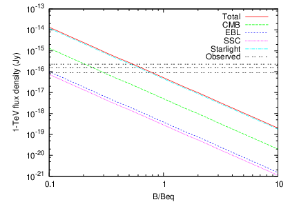
Any departure from equipartition alters the situation significantly. As decreases below , the electron number density and thus inverse-Compton emissivity increase rapidly (Fig. 5). The predicted flux goes roughly as at 1 TeV: so, for the model with discussed above, the HESS data require . In the lobes and hotspots of FRII radio galaxies (e.g. Hardcastle et al. 2004, Kataoka & Stawarz 2004, Croston et al. 2005) we routinely see departures from equipartition at this level, so we do not regard it as at all implausible that the TeV emission really is wholly produced by the kpc-scale jet for . We can also say that models where is more than a factor of a few below are convincingly ruled out by the data, irrespective of , particularly when we consider that many possible other emission processes may contribute to the observed TeV emission (Aharonian et al. 2009) and that our models of the source TeV electron population in Cen A are quite conservative. Stawarz, Kneiske & Kataoka (2006b) reached a similar conclusion based on the FRI source population’s contribution to the -ray background, but this is the first time that TeV emission has been used directly to constrain the magnetic field strength in an individual source.
5.2 M87


The situation is clearly different for the M87 jet. Fig. 6 again shows inverse-Compton emission as a function of angle to the line of sight for our adopted model with . In this model, SSC emission actually dominates over the other photon fields for large , presumably a consequence of the fact that M87’s jet is physically smaller than and significantly more luminous than Cen A’s. The key difference, though, is that the net IC emission does not approach the levels of the 2009 VERITAS flux for : for (the SED for which is plotted in Fig. 7), it is more than two orders of magnitude below the observations, and a departure from equipartition of a factor would be required to bring the flux up to observable levels. Even assuming for the whole jet [as argued by Biretta et al. (1995) for the inner jet only], while retaining , only increases the predicted 1-TeV flux density by a factor . We can again claim to have constrained the field strength from these observations, but it is a much weaker constraint, and our prediction is that the bulk of the TeV emission from M87 must come from some other source unless the angle to the line of sight is very small. One interesting point here is the relative weakness of the starlight component in M87 compared to that Cen A: although the energy density in starlight in M87 is significantly higher than that in the CMB, and this is reflected in the relative normalizations of the peaks in Fig. 7), the starlight contribution actually falls to levels comparable to that of the CMB emission by 1 TeV, whereas ‘starlight’ dominates by a large factor at the same energies in Cen A, as can be seen in Fig. 4. We believe that the reason for this is the very different spectra adopted for the two host galaxies. The ‘starlight’ model in Cen A includes a large contribution from dust emission from the central dust lane, whereas there is no evidence for dust emission from M87 at any significant level (Section 4.2). Klein-Nishina effects significantly reduce the efficiency of scattering of the predominantly optical and near-IR photons from the M87 stellar population into the TeV band. At these energies, a simple comparison of the energy densities of the photon populations is not a reliable guide to their contribution to inverse-Compton emission: this also suggests that strong dust emission may be a pre-requisite for a bright TeV-emitting jet.
6 Prospects for next-generation facilities

The Cerenkov Telescope Array (CTA) is the next-generation TeV gamma-ray facility, currently in the design phase (CTA Consortium 2010). It will both be significantly more sensitive and have significantly higher angular resolution than existing facilities such as HESS and VERITAS. Unfortunately, the likely angular resolution (expected to be arcmin at 1 TeV: e.g. CTA Consortium 2010) is too low to resolve even M87’s kpc-scale jet (with a length in the X-ray of arcsec) from its active nucleus, and the same is true for most other kpc-scale X-ray jets at distances greater than M87’s. The best hope for an observational test of the idea that kpc-scale jets can be responsible for TeV -ray emission will, unsurprisingly, be provided by Cen A. Here the X-ray jet, which extends for arcmin on the sky, should be clearly resolved by the CTA. Unfortunately in our models, in which scattering of starlight dominates the inverse-Compton emission, the jet is still brightest in the unresolved central regions (Fig. 8). However, if we take the model with displayed in (Fig. 8), and assume that all the currently observed VHE emission is produced by the jet, then half the total observed 1-TeV flux density should be produced in the region outside 1 arcmin (1 kpc), and this extended emission should be relatively easy for the CTA to detect, given its greatly improved sensitivity over its predecessors. A moderate-duration observation of Cen A with the CTA will therefore very probably be able to make a conclusive measurement of the magnetic field in an FRI jet for the first time. Even a non-detection would place a lower limit on the magnetic field strength that will be considerably higher than the equipartition value, and would therefore be of great interest as no other component of a radio galaxy for which the magnetic field strength has been measured exhibits this kind of behaviour33 3 There is some evidence that on large scales the energy density in FRI jets is dominated by non-radiating particles — e.g. Croston et al. (2008) — and so it is not completely implausible that the true magnetic field is greater than the field derived by assuming equipartition with the radiating electrons only, but without these CTA observations there will be no way of testing this model by direct observation..
Other than Cen A, the best FRI jets for study with the CTA will be the very few more distant objects with X-ray jets that are extended on several-arcmin – and thus typically 100-kpc – scales. The best example that we are aware of is NGC 6251 (), whose large-scale X-ray jet, starting around 3 arcmin from the nucleus, was first detected with ROSAT (Mack, Kerp & Klein 1997) and later studied in detail with Chandra and XMM (Evans et al. 2005). As discussed in the latter paper, it is not even clear whether the X-ray emission from the 100-kpc scale jet in NGC 6251 is synchrotron in origin, and we do not have a detailed model for the electron spectrum or direct constraints on the jet speed or angle to the line of sight. However, we can make some rough estimates of the detectability of VHE -rays. Using the one-zone synchrotron model presented by Evans et al, we modelled region 1 of the extended jet as a cylinder with a linear radial dependence of electron density and with and , placed it at the appropriate distance from the host galaxy (which we assume for simplicity to have the same SED as M87) and computed the inverse-Compton emission in the VHE -ray band. We find a 1-TeV flux density at equipartition of Jy, a factor below that measured by HESS for Cen A, and compute a predicted photon index of 2.5. The CMB is by a large factor the dominant photon field here – light from the host galaxy, SSC and the EBL all come in an order of magnitude or more lower – and what prevents the TeV emission being much fainter as a consequence is the rather small break inferred by Evans et al. (2005) in the electron energy spectrum for the jet, coupled with its large volume, which means that the bulk of the jet’s luminosity on these scales actually emerges in inverse-Compton in the -ray regime. Although the flux density we estimate here is only one value from the large range that we would obtain if we had the data to carry out more detailed modelling, the fact that it is only about an order of magnitude below what is already measurable for Cen A is encouraging, and suggest that NGC 6251 and any similar objects might provide interesting targets for long exposures with the CTA.
7 Conclusions
The main conclusions from this paper can be summarized as follows:
- 1.
We have developed a framework for carrying out detailed inverse-Compton modelling of the kpc-scale jets of radio galaxies in the regime where the anisotropic nature of inverse-Compton emission and Klein-Nishina effects are important, and applied it to the well-studied jets of Cen A and M87.
- 2.
We have shown that the predicted inverse-Compton flux density in VHE -rays on plausible models of Cen A is quite comparable to what is observed. This means that the existing TeV observations of Cen A put quite strong constraints on the magnetic field strength in the kpc-scale jet, particularly given that we have not modelled either the TeV electrons present in the compact knots in Cen A or the photon field from the presumed hidden blazar in its nucleus: must be comparable to or larger than the equipartition field, unless our beliefs about the probable jet speed or angle to the line of sight are very wrong. This is the first time that a TeV detection of an individual source has been used to put constraints on the jet magnetic field strength; our work supports the analysis of Stawarz et al. (2006b), which was based on the -ray background, in suggesting that the magnetic field in these jets cannot be much less than the equipartition value.
- 3.
Similar but weaker constraints can be derived for M87: it seems likely from our analysis that the large-scale jet contributes only a small fraction of the observed TeV emission from this source, which is consistent with the fact that the TeV emission is seen to be strongly variable. More observational work is needed in this case to pin down a non-variable component which could be compared with our predictions.
- 4.
The prospects for study of extended X-ray jets with future, more sensitive VHE telescopes such as the CTA are limited primarily by the spatial resolution that will be achievable – in many cases kpc-scale jets may be detectable but unresolved from emission related to the AGN or to the pc-scale jet. In Cen A, there is a very realistic possibility of resolving the jet, and we have shown that the possible 100-kpc-scale X-ray synchrotron jet in NGC 6251, which should also be resolved by the CTA, may not be completely out of reach for such instruments. Angular resolution, rather than raw sensitivity, may be the limiting factor for the CTA in the field of extragalactic jets.
Acknowledgements
MJH thanks the Royal Society for a research fellowship. JHC acknowledges support from the South-East Physics Network (SEPNet).
References
- [] Abdo, A.A., et al. [for the Fermi Collaboration], 2010, Sci, 328, 725
- [] Acciari, et al. 2009, Sci, 325, 444
- [] Acciari, et al. 2010, ApJ, 716, 819
- [] Aharonian, F., et al. 2003, A&A, 403, L1
- [] Aharaonian, F., et al. 2009, ApJ, 695, L40
- [] Baes, M., et al. 2010, A&A, 518, L53
- [] Bird, S., Harris, W.E., Blakeslee, J.P., Flynn, C., 2010, A&A, 524, 71
- [] Biretta, J.A., Stern, C.P., Harris, D.E., 1991, AJ, 101, 1632
- [] Biretta, J.A., Zhou, F., Owen, F.N., 1995, ApJ, 447, 582
- [] Brunetti, G., 2000, Astropart. Phys., 13, 107
- [] Cheung, C.C., Harris, D.E., Stawarz, Ł., 2007, ApJ, 663, L65
- [] Croston, J.H., Hardcastle, M.J., Harris, D.E., Belsole, E., Birkinshaw, M., Worrall, D.M., 2005, ApJ, 626, 733
- [] Croston, J.H., Hardcastle, M.J., Birkinshaw, M., Worrall, D.M., Laing, R.A., 2008, MNRAS, 386, 1709
- [] Croston, J.H., et al. 2009, MNRAS, 396, 1999
- [] CTA Consortium, 2010, arXiv:1008.3703
- [] Evans, D.A., Hardcastle, M.J., Croston, J.H., Worrall, D.M., Birkinshaw, M., 2005, MNRAS, 359, 363
- [] Feigelson, E.D., Schreier, E.J., Delvaille, J.P., Giacconi, R., Grindlay, J.E., Lightman, A.P., 1981, ApJ, 251, 31
- [] Ferrarese, L., Mould, J.R., Stetson, P.B., Tonry, J.L., Blakeslee, J.P., Ajhar, E.A., 2007, ApJ, 654, 186
- [] Gilmore, R., Ramirez-Ruiz, E., 2010, ApJ, 721, 709
- [] Goodger, J.L., et al., 2010, ApJ, 708, 675
- [] Hardcastle, M.J., Birkinshaw, M., Worrall, D.M., 2001, MNRAS, 326, 1499
- [] Hardcastle, M.J., Birkinshaw, M., Cameron, R., Harris, D.E., Looney, L.W., Worrall, D.M., 2002, ApJ, 581, 948 [H02]
- [] Hardcastle, M.J., Worrall, D.M., Kraft, R.P., Forman, W.R., Jones, C., Murray, S.S., 2003, ApJ, 593, 169
- [] Hardcastle, M.J., Harris, D.E., Worrall, D.M., Birkinshaw, M., 2004, ApJ, 612, 729
- [] Hardcastle, M.J., Kraft, R.P., Worrall, D.M., 2006, MNRAS, 368, L15
- [] Hardcastle, M.J., et al., 2007, ApJ, 670, L81
- [] Hardcastle, M.J., Cheung, C.C., Feain, I.J., Stawarz, Ł., 2009, MNRAS, 393, 1041
- [] Harris, D.E., Carilli, C.L., Perley, R.A., 1994, Nat, 367, 713
- [] Harris, D.E., Cheung, C.C., Biretta, J.A., Sparks, W.B., Junor, W., Perlman, E.S., Wilson, A.S., 2006, ApJ, 640, 211
- [] Harris, G.L., Rejkuba, M., Harris, W.E., 2010, PASA, 27, 457
- [] Isobe, N., Tashiro, M., Makishima, K., Iyomoto, N., Suzuki, M., Murakami, M.M., Mori, M., Abe, K., 2002, ApJ, 580, L111
- [] Kataoka, J., Stawarz, Ł., 2005, ApJ, 622, 797
- [] Laing, R.A., Bridle, A.H., 2002, MNRAS, 336, 328
- [] Liu, Y., Zhou, X., Ma, J., Wu, H., Yang, Y., Li, J., Chen, J., 2005, AJ, 129, 2628
- [] Mack, K.-H., Kerp, J., Klein, U., 1997, A&A, 324, 870
- [] Mellier, Y., Mathez, G., 1987, A&A, 175, 1
- [] Moskalenko, I.V., Porter, T.A., Strong, A.W., 2006, ApJ, 640, L155
- [] Perlman, E.S., Wilson, A.S., 2005, ApJ, 627, 140
- [] Raue, M., Mazin, D., 2008, Int. J. Mod. Phys. D, 18, 1633
- [] Stawarz, Ł., Sikora, M., Ostrowski, M., 2003, ApJ, 597, 186
- [] Stawarz, Ł., Aharonian, F., Wagner, S., Ostrowski, M., 2006a, MNRAS, 371, 1705
- [] Stawarz, Ł., Kneiske, T.M., Kataoka, J., 2006b, ApJ, 637, 693
- [] Tavecchio, F., Maraschi, L., Sambruna, R.M., Urry, C.M., 2000, ApJ, 544, L23
- [] Worrall, D.M., Birkinshaw, M., Hardcastle, M.J., 2001, MNRAS, 326, L7