Exact diagonalization study of the tunable edge magnetism in graphene

We start from the simplest possible non-interacting tight-binding model of electrons in graphene zigzag ribbons, taking into account only nearest neighbor hoppings of $\pi$ electrons $\mathcal{H}=\sum_{\left<i,j\right>,\sigma}c^{\dagger}_{i\sigma}c_{j\sigma}$, where $\left<i,j\right>$ runs over nearest neighbor sites of a half-infinite honeycomb lattice, $i\equiv(m,n,s)$ is a collective site index for the $(m,n)$th unit cell and the $s=A,B$ sublattice (see Fig. 1), and $c_{i\sigma}$ annihilates an electron at site $i$ with spin $\sigma$. Since we are exclusively interested in the zero energy eigenstates of $\mathcal{H}$, the actual energy scale of $\mathcal{H}$ is unimportant so that we may drop it.¹¹ 1 It is only important to assume that this energy scale is large enough so that the restriction to the zero energy sector of $\mathcal{H}$ is well justified. The validity of this assumption has been checked in Ref. 13. The zero energy states are created by the fermionic edge state operator

where $u_{p}=-1-e^{ip}$, $p$ is the momentum in $m$ direction (along the edge), and $c_{pn\sigma}=L^{-\frac{1}{2}}\sum_{m}e^{-ipm}c_{(m,n,B)\sigma}$, with the number of unit cells $L$ in $m$ direction, i.e., along the edge. The $p$-dependent normalization constant $\mathcal{N}_{p}=\sqrt{2\cos(p-\pi)-1}$ can be interpreted as the weight of the edge state wave function right at the edge atoms where $n=0$. It is easily seen that $\mathcal{H}e^{\dagger}_{p\sigma}=0$. As the edge state wave function is only non-zero on the $B$ sublattice we omit the sublattice index, setting it to $s=B$.

The two most important features of the edge state wave function [Eq. (1)] are : (a) The edge state only exists for momenta $\frac{2\pi}{3}<p<\frac{4\pi}{3}$. In the rest of the Brillouin zone the edge state wave function is not normalizable, as $|u_{p}|>1$ for these momenta. (b) In $n$ direction the edge state is sharply localized at the edge for $p=\pi$, wereas for $p$ close to one of the Dirac points $K=\frac{2\pi}{3}$ and $K^{\prime}=\frac{4\pi}{3}$, the wave function delocalizes into the bulk [see also Fig. 1(b)]. These two edge state properties are stable against adding more details, such as second-nearest neighbor hopping or various edge passivations, to the honeycomb Hamiltonian $\mathcal{H}$.[13, 20] The detailed analysis presented in this paper will clarify that the existence of edge magnetism and in particular its tunability are consequences of these two edge state properties.

The $p$-dependence of the localization length of $\psi_{p}$ has consequences for the edge states’ self-energy $\epsilon_{0}$ as well as for their interaction vertex function $\Gamma$. Neglecting the bulk state contributions,[13] the self-energy correction due to a perturbation $V$, which is invariant along the edge, is given by $\epsilon_{0}(p)=\left<\psi_{p}|V|\psi_{p}\right>$. Due to the delocalization of $\psi_{p}(n)$ for $p$ near $K,K^{\prime}$, edge-localized perturbations $V$ lead to self-energy corrections for which $\epsilon_{0}(K)=\epsilon_{0}(K^{\prime})=0$ while $\epsilon_{0}(\pi)\sim||V||$. For sufficiently well behaved perturbations the self-energy correction gives rise to a smooth edge state energy dispersion with a bandwidth $\Delta\sim||V||$. For a large class of these edge-localized perturbations, the self-energy correction approximately has the form

with $\mathcal{N}_{p}^{2}$ the $p$-dependent weight of the edge state wave function right at the edge. Eq. (2) expresses that an edge state which is more localized at the edge experiences a stronger self-energy correction from an edge-localized perturbation than an edge state which is delocalized into the bulk region. Examples of such perturbations are edge passivations, graphane termination,[20] or local interactions with the substrate. Note that the edge state bandwidth $\Delta$ is experimentally tunable in various ways so that we consider $\Delta$ as a free parameter. Therefore, the noninteracting part of the direct model (dm) edge state Hamiltonian is given by:

where the sum is restricted such that only edge state operators $e_{p\sigma}$ with $\frac{2\pi}{3}\leq p\leq\frac{4\pi}{3}$ appear.

The effective interaction of the edge states, derived by projecting the Hubbard Hamiltonian on the two-dimensional honeycomb lattice $H_{U}=U\sum_{i}c^{\dagger}_{i\uparrow}c_{i\uparrow}c_{i\downarrow}^{\dagger}c_{i\downarrow}$ to the Fock space spanned by the edge states, reads[13]

Together, we have the effective Hamiltonian $H^{\text{dm}}=H_{0}^{\text{dm}}+H_{1}^{\text{dm}}$. The interaction vertex is given by the overlap of the wave functions of all four fermions (with momenta $p+q,p,p^{\prime}-q,p^{\prime}$) participating in the interaction

While the denominator, resulting from the geometric series over $n$, turns out to lead only to unimportant quantitative corrections, the numerator of $\Gamma$, which is the product of the wave function weights at the edge $\mathcal{N}_{p}$ for each of the four fermion operators, leads to the momentum-dependence of the interaction strength which is important for the stability of the weak edge magnetism. Essentially, the effective interaction becomes stronger the more localized the participating fermions are, i.e., the closer their momenta are to $p=\pi$. If one or more of the momenta are close to the Dirac points $\frac{2\pi}{3},\frac{4\pi}{3}$, where the edge state wave functions delocalize into the bulk, the effective interaction is suppressed (see Fig. 1). Note that setting the denominator in Eq. (5) to unity corresponds to assuming that the Hubbard interaction is only present at the outermost line of carbon atoms right at the edge. Such an approximation has been used in Ref. 21. We find that this approximation is inessential for the edge magnetism, leading only to quantitative corrections.

An important consequence of the restriction of the $p$ summation in Eq. (4) is the absence of umklapp processes. As explained above, edge states only exist in one third of the Brillouin zone, i.e. for $\frac{2\pi}{3}\leq p\leq\frac{4\pi}{3}$, so that no four fermion process with momentum $\pm 2\pi$ exists. Indeed, within the restricted Brillouin zone, the process with the largest possible total momentum $p_{\rm tot}$ is $e^{\dagger}_{4\pi/3\uparrow}e_{2\pi/3\uparrow}e^{\dagger}_{4\pi/3\downarrow}e_{2\pi/3\downarrow}$, i.e. $p_{\rm tot}=\frac{4\pi}{3}<2\pi$. Processes with larger total momentum leave the restricted Brillouin zone and are therefore suppressed, as they involve the overlap of edge states and bulk states, which is small. Also, most of the bulk states live in a different energy regime than the edge states.[13]

Thus, we have identified two properties of edge states which make them fundamentally different from usual one-dimensional conductors:

1. (a)

   Due to the restricted Brillouin zone, umklapp processes are forbidden.

2. (b)

   The transverse localization $\mathcal{N}_{p}$ of the edge state wave function gives rise to a tunable band width $\epsilon_{0}(p)\simeq\mathcal{N}_{p}^{2}\Delta$. Furthermore, the interaction vertex becomes weaker if the momenta of the participating fermions approach a Dirac point, i.e. $\Gamma(p,p^{\prime},q)\propto\mathcal{N}_{p+q}\mathcal{N}_{p}\mathcal{N}_{p^{\prime}-q}\mathcal{N}_{p^{\prime}}$.

We will show that these properties are the basis for the magnetism at graphene edges.

We now introduce a generalized model in which the different aspects of the effective electron-electron interaction, found in the previous subsection, may be tuned independently. For this, we map the edge state operators $e_{p,\sigma}$ which correspond to right (left) moving modes for $\pi<p<\frac{4\pi}{3}$ ($\frac{2\pi}{3}<p<\pi$), to fermionic operators $c_{kr\sigma}$ in which $r=R,L$ specifies the direction of motion and $-\frac{\pi}{6}\leq k\leq\frac{\pi}{6}$, i.e. $c_{kr\sigma}=e_{k+\pi+r\pi/6,\sigma}$ and $p=k+\pi+r\pi/6$. The direction of motion $r=R,L$ corresponds to $r=\pm 1$ when used in formulas. Note that the zero point of $k$ has been shifted so that $k=0$ corresponds to $p=\pi\pm\pi/6$ for right and left movers, respectively (see Fig. 2).

For the non-interacting part of the generalized edge state model we assume a linear spectrum with slope $\pm v_{F}$

This linearization of the self-energy [Eq. (2)] only leads to inessential quantitative corrections (see also Appendix B).

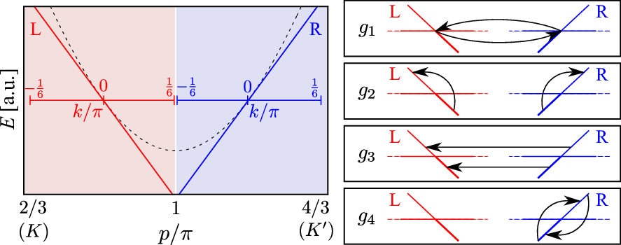
The partitioning into left- and right-movers always gives rise to four terms in the interaction part $H_{1}$ of the Hamiltonian involving different combinations of left- and right-moving modes. Conventionally, these terms are called $g_{1},g_{2},g_{3},g_{4}$ processes (see Fig. 2 and Ref. 22). $g_{2},g_{4}$ correspond to forward scattering, involving processes that scatter only between modes with the same direction of motion, $g_{1}$ refers to backward scattering, and $g_{3}$ are the umklapp terms which are forbidden in edge states. Note that, unlike in usual $g$-ology,[22] we may not assume that the coupling constants for the individual $g_{i}$ processes are constant. The momentum-dependence of the $g_{i}$ must be taken into account.

The two forward scattering processes $g_{2}$ and $g_{4}$ may be merged together into one Hamiltonian²² 2 The equal strength of the $g_{2}$ and $g_{4}$ processes is due to the symmetry property $\Gamma(-k_{F},k_{F},2k_{F})=\Gamma(\pm k_{F},\pm k_{F},0)$, which is a consequence of the origin of $\Gamma$ in the 2D honeycomb Hubbard model (see Ref. 13).

where $:A:$ enforces the normal order[22] of the operator $A$. The primed sum is restricted such that $|k|<\pi/6$ for all momentum arguments $k$ in the electron operators. In order to be able to change the amplitude of the momentum-dependence of the interaction vertex $\Gamma(p,p^{\prime},q)$ [see Eq. (5)], we introduce the factors

from which we build the interaction vertex for the generalized model. The factor $\Gamma_{1}\in[0,6/\pi]$ quantifies the momentum-dependence. For $\Gamma_{1}=0$ the interaction is momentum-independent. This limit corresponds to usual one-dimensional Hubbard chains. For $\Gamma_{1}=6/\pi$ the interaction goes to zero if at least one of the fermions is close to the upper band edge ($k=r\pi/6$). This corresponds to the direct model, where the trigonometric term under the square root in $\mathcal{N}_{p}$ has been replaced by a linear approximation. The differences between the generalized model in the edge state limit and the direct model only lead to quantitative renormalizations of the critical point, as shown in Appendix B. The essential property of the interaction vertex is that it approaches zero if one of the fermion momenta gets close to the Dirac points. This feature is present in the direct and in the generalized model with $\Gamma_{1}=6/\pi$.

The form of the backscattering $(g_{1})$ Hamiltonian $H_{1}^{\rm bs}$ is similar to $H_{1}^{\rm fs}$. However the scattering takes place between left- and right-movers

We have introduced the additional parameter $\lambda_{\rm bs}$ which allows us to tune the overall strength of the $g_{1}$ processes relative to the $g_{2},g_{4}$ processes. $\lambda_{\rm bs}=1$ corresponds to the physical backscattering strength which is required by SU(2) invariance.[22] Nevertheless, we will investigate the consequences of a suppression of backscattering since this will be important for a bosonization analysis of the generalized model which will be presented in an upcoming paper.[24]

As already pointed out, an important feature of edge states is the absence of umklapp processes in the effective electron-electron interaction. However, in order to be able to compare the edge state model to a Hubbard chain, we add an artificial umklapp process with relative strength $\lambda_{\rm us}$ to the Hamiltonian of the generalized model

Varying $\lambda_{\rm us}$ between 1 (Hubbard chain limit) and 0 (edge state limit) allows us to investigate the consequences of the presence of umklapp processes for one-dimensional ferromagnetism.

Alltogether, the four parameters $v_{F}/U$, $\lambda_{\rm bs}$, $\lambda_{\rm us}$, and $\Gamma_{1}$ define the phase space of the generalized model

The following limits of this model may be identified:

1. 1.

   Edge state limit: the generalized model with the parameters $\lambda_{\rm bs}=1$, $\lambda_{\rm us}=0$, and $\Gamma_{1}=6/\pi$, is a good approximation of the direct model.

2. 2.

   Hubbard chain limit: for $\lambda_{\rm bs}=1$, $\lambda_{\rm us}=1$, and $\Gamma_{1}=0$, the generalized model essentially describes a one-dimensional Hubbard chain. The only difference is the assumption of a linearized single-particle spectrum instead of the $2\cos(k)$ dispersion.

Note that it is important to work in the k-space formulation because it is difficult to control the umklapp scattering or the momentum dependence of the interaction vertex in a real space formulation. One reason for this is that an interaction vertex $\Gamma(p,p^{\prime},q)$ with a nontrivial $p,p^{\prime}$ dependence does not transform to a real space interaction of the form $V(x-x^{\prime})$ but to a complicated non-local interaction. This also hampers the application of DMRG methods to this problem.

First we study the crossover from a usual Hubbard chain to interacting edge states. As explained above, the generalized model can be tuned continuously between these two limiting cases by means of the parameters $\lambda_{\rm us}$ and $\Gamma_{1}$. We postpone the analysis of backscattering to the next subsection and set $\lambda_{\rm bs}=1$ here.

It is most instructive to begin with the Hubbard chain limit of the generalized model, which is characterized by the full umklapp process strength $\lambda_{\rm us}=1$ and a suppressed momentum dependence of the interaction $\Gamma_{1}=0$. With this parameter set the direct model resembles a one-dimensional metal with a linear single particle dispersion instead of a cos-dispersion. ⁴⁴ 4 We have checked that the linearization of the single particle spectrum does not change the results qualitatively. The lowest eigen energies in the different $S_{z}$ subspaces for the parameter set described above are shown in Fig. 3. Obviously, the ground state is non-degenerate and resides in the $S_{z}=0$ subspace for arbitrary $v_{F}\pi/U$, except for the limit of infinitely large $U$. Thus, as expected, no ferromagnetic phase transition exists for the Hubbard chain limit of the generalized model at finite $v_{F}\pi/U$, in consistence with the Lieb-Mattis theorem[14] which states that the ground state of a system of one-dimensional interacting electrons has zero total spin and is non-degenerate with higher spin subspaces. ⁵⁵ 5 The point $v_{F}\pi/U=0$ corresponds to a pathologic potential in Ref. 14, as it can be reached by $U\rightarrow\infty$. At this point, all sectors with total spin $0\leq S\leq S_{\text{max}}$ are degenerate.

Next, the generalized model is tuned away from the Hubbard chain limit by suppressing the umklapp scattering $\lambda_{\rm us}<1$. Suppressed umklapp scattering is one of the properties of edge states which makes them fundamentally different from usual one-dimensional metals. In the inset of Fig. 3, the lowest eigen energies of the $S_{z}=0$ and the $S_{z}=\pm N/2$ (full spin-polarization) subspaces are shown as $\lambda_{\rm us}$ is reduced from 1 to 0 in steps of 0.2. For any $\lambda_{\rm us}<1$ there is a nonzero critical value for $v_{F}\pi/U$ below which the lowest energy states of these two subspaces and also for all $S_{z}$ in between (not shown in the inset of Fig. 3) are equal. This corresponds to a high spin state of size $S=6$ in which the spins of all electrons point into the same direction. The critical point at which the transition between $S=0$ and $S=N/2$ takes place depends on the umklapp scattering strength

For $N=12$ we find for the exponent $y\simeq 0.5\pm 0.02$. Obviously, the absence of umklapp scattering allows a high spin ground state. However, for $\lambda_{\rm us}<1$ and $\Gamma_{1}=0$, the system instantly jumps from zero polarization $S=0$ to the maximal possible polarization $S=N/2$ at the critical point $[v_{F}\pi/U]_{\rm crit.}^{(\Gamma_{1}=0)}$. This is a first order phase transition. For the case of completely suppressed umklapp scattering $\lambda_{\rm us}=0$ this is shown in Fig. 4 (a), where the lowest eigen energies of all subspaces are plotted as a function of $v_{F}\pi/U$: the $S_{z}=0$ subspace contains the non-degenerate ground state until at the critical point the lowest energy eigenstates of all subspaces form the degenerate ground state; no intermediate regime of $v_{F}\pi/U$ exists in which there is only a degeneracy between some of the $S_{z}$ subspaces.

The reason for the instant jump in the total spin is as follows: once the Stoner criterion $v_{F}\pi/U>[v_{F}\pi/U]^{(\Gamma_{1}=0)}_{\rm crit.}$ is met, the interaction energy gain $\delta E_{U}(S)$ associated with developing a certain spin polarization $S$ is larger than the corresponding kinetic energy penalty $\delta E_{\rm kin}(S)$. Unlike in two or three dimensions, however, for one-dimensional systems with momentum-independent interactions, $\delta E(S)=\delta E_{U}(S)+\delta E_{\rm kin}(S)$ has no minimum, i.e. $\delta E(S+1)<\delta E(S)$, for all $S<S_{\rm max}$. Thus, the system instantly ’flows’ to the highest possible polarization $S_{\rm max}$, once the Stoner criterion is met. This is a rather common feature of one-dimensional systems with a constant interaction vertex (such as the Hubbard interaction) and can easily be observed in a variational calculation of the ground state properties (see Appendix A).

The momentum-dependence of the interaction vertex ($\Gamma_{1}>0$) reduces the interaction energy gain as the spin-polarization $S$ becomes larger. This is because for larger $S$, the Fermi level of the spin-up right-movers is shifted to higher momenta where the interaction is suppressed by the $S^{r=R}_{k}$ factors [see Eq. (7)]. Similarly, for the spin-up left-movers, the Fermi level is then shifted to smaller momenta, where the $S^{r=L}_{k}$ suppress the interaction.⁶⁶ 6 Note that the increase in the interaction vertex for the spin-down electrons with lowered Fermi level is overcompensated by the suppression due to the higher Fermi level of the spin-up electrons, so that in total the interaction is reduced as $S$ grows. As a result, $\delta E(S)$ develops a minimum at $S=S_{\rm min}<S_{\rm max}$, and the system is stable there. Intuitively, this may be understood on the basis of a variational calculation (see Appendix A). Within exact diagonalization one finds that with $\Gamma_{1}=6/\pi$, the ground state degeneracy increases successively from 0 to $2S_{\rm max}+1$ by first adding the lowest energy eigenstates of the $S_{z}=\pm 1$ subspaces to the ground space, and then the $S_{z}=\pm 2$ subspaces and so forth. This is shown in Fig. 4 (b).

If the total spin $S$ is plotted as a function of $v_{F}\pi/U$, $S$ decreases from $S_{\rm max}$ to 0 in steps. These steps correspond to the positions $v_{F}\pi/U$, where the degree of the ground state degeneracy changes, indicated by arrows in Fig. 4. For $\Gamma_{1}=0$, there is one step where the spin-polarization jumps from $S=S_{\rm max}=N/2$ to $S=0$, while for the maximal $\Gamma_{1}=6/\pi$, there are $N/4$ steps at each of which the spin-polarization is decreased by $\Delta S=2$.⁷⁷ 7 This decrease of $2$ in $S$ is due to the contribution of the left- and right-moving branch to the spin-polarization: each branch contributes one spin flip. Fig. 5 shows these two limiting cases and how the steps evolve as $\Gamma_{1}$ is varied from 0 to $6/\pi$. The momentum-dependence must have a minimum strength $\Gamma_{1}>\Gamma_{1}^{c}\simeq 1$, in order to break the one big spin- polarization step of height $N/2$ into many small steps of height 2. Thus, for $\Gamma_{1}>\Gamma_{1}^{c}$ there is a regime of weak edge magnetism, meaning that the total spin $S$ of the ground state is smaller than the maximal spin $S_{\text{max}}$, in addition to the usual saturated edge magnetism for small $v_{F}\pi/U$ (i.e. $S=S_{\text{max}}$) and the Luttinger liquid regime for large $v_{F}\pi/U$ with $S=0$. Figure 6 shows a diagram in which the phase boundaries between the Luttinger liquid (LL), the saturated edge magnetism (SEM) and the novel weak edge magnetism (WEM) are shown for different system sizes $N=8,12,16$.

Note that the non-zero $\Gamma_{1}^{c}$ found in the exact diagonalization reveals a weakness of the fermionic mean-field theory in which this minimum momentum dependence, above which a WEM regime appears, is zero (see Appendix A). A non-zero $\Gamma_{1}^{c}$ means that the small momentum-dependencies which always follow from a dependence of the Bloch wave functions in usual one-dimensional conductors on the momentum are not necessarily sufficient to stabilize the weak edge magnetism; the momentum-dependence of the interaction vertex must be sufficiently strong for this.

In the limit $L\rightarrow\infty$, which cannot be accessed within exact diagonalization, of course, $S/S_{\rm max}$ becomes a smooth function of $v_{F}\pi/U$. We approximate this smooth function by a power law

Fermionic mean-field theory (see Appendix A) predicts $\beta=0.5$. Because the exact diagonalization study is limited to small systems $N\leq 16$, it is difficult to obtain a decent estimate of the exact exponent $\beta$ within this work. Fitting the edge state limit of the generalized model to the center of the plateaus of the $N=16$ results of the exact diagonalization, we obtain $0.44<\beta<0.61$, dependent on how many plateaus are included in the fit. The critical point $\left(\frac{v_{F}\pi}{U}\right)_{\rm crit.}\simeq 0.760$ for this fit is obtained by extrapolating the rightmost step from the data sets $N=4,8,12,16$ to $N=\infty$.

Interestingly, $\Gamma_{1}$ not only affects the order of the transition but also the critical $v_{F}\pi/U$. This is also not correctly predicted by the mean-field approach (see Appendix A), which, independently of $\Gamma_{1}$, finds $v_{F}\pi/U=1$ to be the critical point. For small $\Gamma_{1}$ and $N=16$ the exact diagonalization gives

For the maximal $\Gamma_{1}=6/\pi$, the position of the leftmost step can be calculated by exact diagonalization for very large systems.[18] We performed calculations for system sizes up to $L=180$ in order to extrapolate this step position. Within the limits of the accuracy of this extrapolation, the critical point $v_{F}\pi/U=0.5\pm 0.001$ between the SEM and the WEM regime coincides with the mean-field prediction (see Appendix A). This extrapolation to the thermodynamic limit, in combination with the extrapolation of the critical point between the WEM and the LL regime, is a strong evidence for the existence of the WEM phase for $0.5\leq v_{F}\pi/U\leq 0.760$ in the thermodynamic limit.

For completeness we note that our exact diagonalization analysis shows that a SEM phase also exists in the general model with umklapp scattering $\lambda_{\rm us}=1$ if $\Gamma_{1}>0$. However even for $\Gamma_{1}=6/\pi$ there is no weak edge magnetism phase between the Luttinger liquid and the saturated edge magnetism as long as $\lambda_{\rm us}=1$.

The backscattering Hamiltonian $H_{1}^{\rm bs}$ is important for the SU(2) invariance of the Hamiltonian. It is easily seen that only for $\lambda_{\rm bs}=1$ the SU(2) symmetry is preserved. At real graphene edges, of course, the backscattering cannot be tuned experimentally. Nevertheless it is interesting to study the consequences of a suppression of $H_{1}^{\rm bs}$ since in a bosonization treatment of the generalized model $H_{1}^{\rm bs}$ translates to a sine-Gordon term which is difficult to analyze. Therefore, some insight into the relevance of $H_{1}^{\rm bs}$ is helpful from a theoretical point of view. Following the philosophy of the previous subsection, we restrict the discussion to the spin polarization properties of the ground state. The analysis of more complicated observables such as spin-spin correlation functions is beyond the scope of this work and will be discussed in another paper.

Fig. 7 compares the lowest eigen energies of the $S_{z}$ subspaces from calculations with and without backscattering. The most striking feature of the suppression of backscattering is the lifting of the ground state degeneracy in the SEM regime. This effect is easily understood by noting that the very reason for the ground state degeneracy in the $\lambda_{\rm bs}=1$ case was the SU(2) symmetry, which, however, is broken for $\lambda_{\rm bs}<1$. Interestingly, the lifting of the degeneracy is such that the lowest energy states of the subspaces with highest $|S_{z}|$, in the ground space for $\lambda_{\rm bs}=1$, form the ground state for $\lambda_{\rm bs}<1$. This means that suppressing backscattering introduces an Ising anisotropy along the spin quantization axis chosen in the definition of the model.

Apart from this degeneracy lifting, the evolution of the ground state properties with $v_{F}\pi/U$ is very similar for calculations with and without backscattering. The positions of the highest spin-polarization steps are practically unchanged. Only at the steps close to the phase transition between the LL and the WEM regime, a deviation of the $\lambda_{\rm bs}=0$ results from the $\lambda_{\rm bs}=1$ results can be observed. A handwaving explanation of this behavior can be given in terms of the bosonization analysis of the WEM regime in Ref. 13. As soon as the Fermi levels for the up-spin electrons and the down-spin electrons are split, the backscattering process for electrons right at the Fermi surface is forbidden because it is not momentum-conserving. Thus, in order to conserve momentum, the electrons are forced to scatter to higher energies if there is a non-zero spin-polarization. This mechanism suppresses the backscattering. In the bosonization language the backscattering Hamiltonian acquires a spatially oscillating phase which makes the corresponding operator irrelevant in the renormalization group. Thus in the WEM regime, not too close to the critical point, $H^{\rm bs}_{1}$ is suppressed and does not give an important contribution.

Close to the critical point, however, Fig. 7 indicates that $H^{\rm bs}_{1}$ becomes more important. This observation is consistent with the qualitative bosonization argument: Close to the critical point the phase oscillations in the bosonic backscattering Hamiltonian get slower until they completely disappear at the critical point.

References

- [1] K. S. Novoselov, A. K. Geim, S. V. Morozov, D. Jiang, Y. Zhang, S. V. Dubonos, I. V. Grigorieva, and A. A. Firsov, Science 306, 666 (2004)
- [2] A. H. Castro Neto, F. Guinea, N. M. R. Peres, K. S. Novoselov, and A. K. Geim, Rev. Mod. Phys. 81, 109 (Jan 2009)
- [3] C. Lee, X. Weil, J. W. Kysar, and J. Hone, Science 321, 385 (2008)
- [4] Y. Zhang, Y.-W. Tan, H. L. Stormer, and P. Kim, Nature 438, 201 (Nov 2005), ISSN 0028-0836, http://dx.doi.org/10.1038/nature04235
- [5] K. S. Novoselov, A. K. Geim, S. V. Morozov, D. Jiang, M. I. Katsnelson, I. V. Grigorieva, S. V. Dubonos, and A. A. Firsov, Nature 438, 197 (Nov 2005), ISSN 0028-0836
- [6] M. Fujita, K. Wakabayashi, K. Nakada, and K. Kusakabe, Journal of the Physical Society of Japan 65, 1920 (1996), http://jpsj.ipap.jp/link?JPSJ/65/1920/
- [7] Y.-W. Son, M. L. Cohen, and S. G. Louie, Phys. Rev. Lett. 97, 216803 (Nov 2006)
- [8] Y.-W. Son, M. L. Cohen, and S. G. Louie, Nature 444, 347 (2007)
- [9] J. Jung and A. H. MacDonald, Phys. Rev. B 79, 235433 (Jun 2009)
- [10] H. Feldner, Z. Y. Meng, A. Honecker, D. Cabra, S. Wessel, and F. F. Assaad, Phys. Rev. B 81, 115416 (Mar 2010)
- [11] H. Feldner, Z. Y. Meng, T. C. Lang, F. F. Assaad, S. Wessel, and A. Honecker, “Dynamical signatures of edge-state magnetism on graphene nanoribbons,” (2011), arXiv:1101.1882
- [12] T. Hikihara, X. Hu, H.-H. Lin, and C.-Y. Mou, Phys. Rev. B 68, 035432 (Jul 2003)
- [13] M. J. Schmidt and D. Loss, Phys. Rev. B 82, 085422 (Aug 2010)
- [14] E. Lieb and D. Mattis, Phys. Rev. 125, 164 (Jan 1962)
- [15] C. Lanczos, J. Res. Nat. Bur. Stand. 45, 255 (1950)
- [16] E. Dagotto, Rev. Mod. Phys. 66, 763 (Jul 1994)
- [17] D. Sénéchal, “An introduction to quantum cluster methods,” (2008), arXiv:0806.2690v2
- [18] At filling, and , we could access edges of length with a dimension of the corresponding Hilbert space of after exploiting all symmetries. For nearly maximal and filling, we were able to calculate the groundstate energy of an edge with length with a Hilbert space dimension of only . In this case we were limited only by the 64 bit limit of the internal storage of the basis vectors and longer edges are in principle accessible by a modification of our code.
- [19] It is only important to assume that this energy scale is large enough so that the restriction to the zero energy sector of is well justified. The validity of this assumption has been checked in Ref. \rev@citealpnumtem_schmidt_loss_2010.
- [20] M. J. Schmidt and D. Loss, Phys. Rev. B 81, 165439 (Apr 2010)
- [21] M. Hohenadler, T. C. Lang, and F. F. Assaad(2011), arXiv:1011.5063
- [22] T. Giamarchi, Quantum Physics in One Dimension (Oxford Univ. Press, 2003)
- [23] The equal strength of the and processes is due to the symmetry property , which is a consequence of the origin of in the 2D honeycomb Hubbard model (see Ref. \rev@citealpnumtem_schmidt_loss_2010).
- [24] M. J. Schmidt(2011)
- [25] An edge with unit cells in length corresponds to only k-space points in the reduced Brillouin zone in which the edge states are defined.
- [26] We have checked that the linearization of the single particle spectrum does not change the results qualitatively.
- [27] The point corresponds to a pathologic potential in Ref. \rev@citealpnumlieb_mattis, as it can be reached by . At this point, all sectors with total spin are degenerate.
- [28] Note that the increase in the interaction vertex for the spin-down electrons with lowered Fermi level is overcompensated by the suppression due to the higher Fermi level of the spin-up electrons, so that in total the interaction is reduced as grows.
- [29] This decrease of in is due to the contribution of the left- and right-moving branch to the spin-polarization: each branch contributes one spin flip.
- [30] S. Daul, Eur. Phys. J. B 14, 649 (2000)
- [31] S. Daul and R. M. Noack, Phys. Rev. B 58, 2635 (1998)