Fibered knots and potential counterexamples to the Property 2R and Slice-Ribbon ConjecturesThanks: Research partially supported by National Science Foundation grants. Thanks also to Mike Freedman and Microsoft’s Station Q for rapidly organizing a mini-conference on this general topic.
Abstract.
If there are any -component counterexamples to the Generalized Property R Conjecture, a least genus component of all such counterexamples cannot be a fibered knot. Furthermore, the monodromy of a fibered component of any such counterexample has unexpected restrictions.
The simplest plausible counterexample to the Generalized Property R Conjecture could be a -component link containing the square knot. We characterize all two-component links that contain the square knot and which surger to . We exhibit a family of such links that are probably counterexamples to Generalized Property R. These links can be used to generate slice knots that are not known to be ribbon.
1. Introduction
Recall the famous Property R theorem, proven in a somewhat stronger form by David Gabai [Ga1]:
Theorem 1.1 (Property R).
If -framed surgery on a knot yields then is the unknot.
Problem 1.82 in Kirby’s problem list [Ki2] conjectures a generalization to links: If surgery on an -component link yields the connected sum then becomes the unlink after suitable handle slides. (See the next section for further discussion.) Although this Generalized Property R Conjecture can be traced back more than two decades, it seems that no progress has appeared in the literature until now. The present paper studies the conjecture, focusing on the case of 2-component links. We conclude that the conjecture is probably false, and analyze potential counterexamples. These examples have relevance to the Slice-Ribbon Conjecture. We also propose a weaker version of the Generalized Property R Conjecture that seems much more likely, and is related to the 4-dimensional smooth Poincaré Conjecture.
We concentrate on links where is fibered. Critical to the argument are developments in sutured manifold theory, developments that go beyond those used by Gabai in his original proof of Property R. In particular we use sutured manifold theory to show (Theorem 3.3) that any counterexample of this form to the Generalized Property R Conjecture generates another 2-component counterexample for which one component has smaller genus than . With this motivation, we assume has genus 2. We then use Heegaard theory to completely characterize such links satisfying the hypothesis of the Generalized Property R Conjecture (Corollary 5.4): After handle slides, is a special type of curve lying on the fiber of . For the simplest plausible , namely the square knot, this characterization becomes simple enough (Corollary 6.4) to allow enumeration of all examples up to handle slides.
2pt \pinlabel at 95 200 \pinlabel at 338 203 \pinlabel at 25 112 \pinlabel at 410 115 \endlabellist
We then use classical 4-manifold theory (the 20-year old paper [Go1] of the first author) to argue that the square knot probably does lie in counterexamples to the Generalized Property R Conjecture. The link in Figure 1 consists of a square knot interleaved with the connected sum of an torus knot with its mirror. (Each summand is depicted as an -stranded spiral, with a full -twist added relative to the plane of the paper. The dotted arc connecting the components will be used momentarily.) We show in Section 7 that is a counterexample to the Generalized Property R Conjecture provided that the presentation
of the trivial group is Andrews-Curtis nontrivial, as is deemed likely by group theorists when . We will see (Section 8) that this link and its generalizations (Figure 14) are necessarily slice, so we can generate slice knots just by band-summing the two components together. For there is no apparent reason for the resulting knots to be ribbon. Thus, we obtain potential counterexamples to the Slice-Ribbon Conjecture. This appears to be the only known method for constructing such examples. Figure 2 shows a simple potential counterexample obtained from by the band-move following the dotted arc in Figure 1.
2pt
\pinlabel at 22 112
\pinlabel at 407 115
\endlabellist
The 4-dimensional viewpoint that discredits the Generalized Property R Conjecture also shows how to rescue it by allowing more moves. In Section 9 we discuss this more plausible version of the conjecture, and its close connection with the 4-dimensional smooth Poincaré Conjecture. Since the key new move is somewhat mysterious, Section 10 shows explicitly how it works to trivialize our potential counterexamples . The main result, Proposition 10.1, can in principle be used to construct other potential counterexamples.
Unless explicitly stated otherwise, all manifolds throughout the paper will be smooth, compact and orientable.
2. Handle slides and Generalized Property R
To make sense of how Property R might be generalized, recall a small bit of -manifold handlebody theory [GS]. Suppose is a link in a -manifold and each component of is assigned a framing, that is a preferred choice of cross section to the normal circle bundle of the component in . For example, if , a framing on a knot is determined by a single integer, the algebraic intersection of the preferred cross-section with the longitude of the knot. (In an arbitrary -manifold a knot may not have a naturally defined longitude.) Surgery on the link via the framing is standard Dehn surgery, though restricted to integral coefficients: a regular neighborhood of each component is removed and then reattached so that the meridian is identified with the cross-section given by the framing. Associated to this process is a certain -manifold: attach -dimensional -handles to along , using the given framing of the link components. The result is a -dimensional cobordism, called the trace of the surgery, between and the -manifold obtained by surgery on . The collection of belt spheres of the -handles constitute a link called the dual link; the trace of the surgery on can also be viewed as the trace of a surgery on .
The -manifold trace of the surgery on is unchanged if one -handle is slid over another -handle. Such a handle slide is one of several moves allowed in the Kirby calculus [Ki1]. When the -handle corresponding to the framed component of is slid over the framed component of the effect on the link is to replace by the band sum of with a certain copy of , namely the copy given by the preferred cross-section realizing the framing of . If and the framings of and are given by the integers and , respectively, then the integer for will be where denotes the linking number and the sign is precisely when the orientations of and the copy of fit together to orient . (This requires us to orient and , but the answer is easily seen to be independent of the choice of orientations.) The terms handle addition and subtraction are used to distinguish the two cases of sign ( and , respectively) in the formula. Any statement about obtaining -manifolds by surgery on a link will have to take account of this move, which we continue to call a handle-slide, in deference to its role in -dimensional handle theory.
Suppose is obtained from components and by the handle-slide of over as described above. Let and be the dual knots to and . It will be useful to note this counterintuitive but elementary lemma:
Lemma 2.1.
The link in that is dual to is , where is obtained by a handle-slide of over .
Proof.
It suffices to check this for the simple case in which the -manifold is a genus handlebody, namely a regular neighborhood of , , and the arc between them along which the band-sum is done. A sketch of this is shown in Figure 3. The dual knots , and are displayed as boundaries of meridian disks for regular neighborhoods of , and respectively.
2pt \pinlabel at 390 543 \pinlabel at 100 543 \pinlabelslide at 171 512 \pinlabel at 465 500 \pinlabel at 90 435 \pinlabel at 380 435 \pinlabel at 245 545 \pinlabel at 225 435 \endlabellist
Alternatively, a -dimensional schematic of the -dimensional process is shown in Figure 4. The handle corresponding to is shown half-way slid across the handle corresponding to . Each disk in the figure is given the same label as its boundary knot in or as appropriate. ∎
2pt
\pinlabel at 37 183
\pinlabel at 137 86
\pinlabelslide at 346 168
\pinlabel at 238 122
\pinlabel at 162 238
\pinlabel at 310 50
\pinlabel at 396 101
\endlabellist
Let denote the connected sum of copies of . The Generalized Property R conjecture (see [Ki2, Problem 1.82]) says this:
Conjecture 1 (Generalized Property R).
Suppose is an integrally framed link of components in , and surgery on via the specified framing yields . Then there is a sequence of handle slides on that converts into a -framed unlink.
In the case no slides are possible, so Conjecture 1 does indeed directly generalize Theorem 1.1. On the other hand, for it is certainly necessary to include the possibility of handle slides. Figure 5 shows an example of a more complicated link on which -framed surgery creates . To see this, note that the Kirby move shown, band-summing the square knot component to a copy of the unknotted component, changes the original link to the unlink of two components, for which we know surgery yields . Even more complicated links with this property can be obtained, simply by using Kirby moves that complicate the link rather than simplify it. See Figure 6; the free ends of the band shown can be connected in an arbitrarily linked or knotted way.
2pt \pinlabel at 72 89 \pinlabel at 137 120 \pinlabel at 281 18 \pinlabel at 338 120 \pinlabel at 432 18 \pinlabel at 432 120 \pinlabelband sum here at 108 -11

The conjecture can be clarified somewhat by observing that the only framed links that are relevant are those in which all framings and linking numbers are trivial. There is a straightforward -dimensional proof, using the intersection pairing on the trace of the surgery. Here is an equally elementary -dimensional proof:
Proposition 2.2.
Suppose is a framed link of components in , and surgery on via the specified framing yields . Then the components of are algebraically unlinked and the framing on each component is the -framing.
Proof.
It follows immediately from Alexander duality that In particular, filling in the solid tori via whatever framing we are given yields an epimorphism, hence an isomorphism . For each torus component of , the filling will kill some generator of , so the homomorphism is not injective. It follows that the homomorphism cannot be injective and, moreover, must contain the framing curve. But must be contained in the subgroup generated by the standard longitude, since this is the only subgroup that is trivial when the other components of are just left in place and not removed from . It follows that the framing at each component is that of the standard longitude, namely the -framing. Since the longitude of each is null-homologous in it follows that all linking numbers are trivial. ∎
There is also an immediate topological restriction on the link itself, which carries over to a restriction on the knots that can appear as individual components of such a link (see [Hi, Theorem 2]):
Proposition 2.3 (Hillman).
Suppose is a framed link of components in , and surgery on via the specified framing yields . Then bounds a collection of smooth -disks in a -dimensional homotopy ball bounded by .
It follows from Freedman’s proof of the -dimensional topological Poincaré Conjecture [Fr] that (and so each component of ) is topologically slice in . See also the earlier [KM] for the case .
Proof.
Consider the -manifold trace of the surgery on . has one end diffeomorphic to and the other end, call it , diffeomorphic to . has the homotopy type of a once-punctured . Attach to via the natural identification . The result is a homotopy -ball, and the cores of the original -handles that are attached to are the required -disks. ∎
Somewhat playfully, we can turn the Generalized Property R Conjecture, which is a conjecture about links, into a conjecture about knots, and also stratify it by the number of components, via the following definition and conjecture.
Definition 2.4.
A knot has Property nR if it does not appear among the components of any -component counterexamples to the Generalized Property R conjecture. That is, whenever is a component of an n-component link and some integral surgery on produces , then there is a sequence of handle slides on that converts into a -framed unlink.
Conjecture 2 (Property nR Conjecture).
All knots have Property nR.
Thus the Generalized Property R conjecture is that the Property nR Conjecture is true for all . Following Proposition 2.3 any non-slice knot has Property nR for all . The first thing that we will show (Theorem 3.3) is that if there are any counterexamples to Property 2R, a least genus such example cannot be fibered. We already know that both of the genus one fibered knots (the figure 8 knot and the trefoil) cannot be counterexamples, since they are not slice, and we show below (Proposition 3.2) that the unknot cannot be a counterexample. So these simplest of fibered knots do have Property 2R. These considerations suggest that, if one is searching for a potential counterexample to Property nR and hope to exploit a knot’s geometric properties, the simplest candidate could be the square knot, viewed as a potential counterexample to Property 2R. After all, the square knot is symmetric, slice, fibered, and both its genus and its crossing number are low.
In fact it turns out that there is a relatively simple range of possibilities for what a -component link containing the square knot and surgering to can look like. The background for this comes from the theory of Heegaard splittings and is discussed in Sections 4 and 6. In Section 7 we present strong evidence that Property 2R does indeed fail for the square knot. Since the square knot is fibered, it would then follow from Theorem 3.3 that there is a counterexample to Property 2R among genus one knots.
On the other hand, the square knot may well satisfy a somewhat weaker property, which is still useful in the connection of Property R to such outstanding -manifold questions as the smooth Poincaré Conjecture and the smooth Schoenflies Conjecture. For this weaker property, copies of canceling Hopf pairs may be added to the link before the handle slides and then removed after the handle slides. Beyond our specific example, we discuss the mechanics of how addition and later removal of a Hopf pair can be used to reduce the complexity of a surgery description.
3. Special results for Property 2R
Almost nothing is known about Generalized Property R, beyond the elementary facts noted in Propositions 2.2 and 2.3 that the framing and linking of the components of the link are all trivial and the links themselves are slice in a possibly exotic ball. A bit more is known about Property 2R. The first proposition was shown to us by Alan Reid:
Proposition 3.1 (A. Reid).
Suppose is a -component link with tunnel number . If surgery on gives then is the unlink of two components.
Proof.
The assumption that has tunnel number means that there is a properly embedded arc so that is a genus handlebody . Let . There is an obvious epimorphism (fill in a meridian disk of ) and an obvious epimorphism (fill in solid tori via the given framing). But any epimorphism is an isomorphism, since free groups are Hopfian, so in fact . It is then a classical result that must be the unlink of two components. ∎
This first step towards the Property 2R conjecture is a bit disappointing, however, since handle-slides (the new and necessary ingredient for Generalized Property R) do not arise. In contrast, Figure 5 shows that handle slides are needed in the proof of the following:
Proposition 3.2.
The unknot has Property 2R.
Proof.
Suppose is the union of two components, the unknot and another knot , and suppose some surgery on gives . Following Proposition 2.2 the surgery is via the -framing on each and, since is the unknot, -framed surgery on alone creates . Moreover, the curve that is dual to is simply for some point .
A first possibility is that is a satellite knot in , so lies in a solid torus in such a way that the torus is essential in . Since there is no essential torus in , compresses after the surgery on . Since contains no summand with finite non-trivial homology, it follows from the main theorem of [Ga3] that is a braid in and that surgery on has the same effect on as some surgery on . Proposition 2.2 shows that the surgery on must be along a longitude of , but that would imply that has winding number in . The only braid in a solid torus with winding number is the core of the solid torus, so in fact is merely a core of and no satellite. So we conclude that cannot be a satellite knot.
Consider the manifold . If it is irreducible, then it is a taut sutured manifold (see, for example, [Ga1]) and two different fillings (trivial vs. -framed) along yield reducible, hence non-taut sutured manifolds. This contradicts [Ga2]. We conclude that is reducible. It follows that is isotopic in to a knot lying in a -ball in and that surgery on creates a summand of the form . By Property R, we know that is the unknot in . Hence is the unlink of two components.
The proof, though, is not yet complete, because the isotopy of to in may pass through . But passing through can be viewed as band-summing to the boundary of a meridian disk of in . So the effect back in is to replace with the band sum of with a longitude of . In other words, the knot , when viewed in , is obtained by from by a series of handle slides over , a move that is permitted under Generalized Property R. ∎
In a similar spirit, the first goal of the present paper is to prove a modest generalization of Proposition 3.2. A pleasant feature is that, since the square knot is fibered, Figure 6 shows that the proof will require handle slides of both components of the link.
Theorem 3.3.
No smallest genus counterexample to Property 2R is fibered.
Proof.
Echoing the notation of Proposition 3.2, suppose there is a -component counterexample to Generalized Property R consisting of a fibered knot and another knot . Let be the -manifold obtained by -framed surgery on alone; will play the role that played in the proof of Proposition 3.2. Since is a fibered knot, fibers over the circle with fiber , a closed orientable surface of the same genus as . The dual to in is a knot that passes through each fiber exactly once.
The hypothesis is that -framed surgery on creates . Following [ST, Corollary 4.2], either the knot lies in a ball, or is cabled with the surgery slope that of the cabling annulus, or can be isotoped in to lie in a fiber, with surgery slope that of the fiber. If were cabled, then the surgery on would create a Lens space summand, which is clearly impossible in . If can be isotoped into a ball or into a fiber, then, as argued in the proof of Proposition 3.2, the isotopy in is realized in by handle-slides of over , so we may as well regard as lying either in a ball that is disjoint from or in a fiber . The former case, in a ball disjoint from would, as in Proposition 3.2, imply that the link is the unlink. So we can assume that .
The surgery on that changes to has this local effect near : is cut open along , creating two copies of , a -handle is attached to the copy of in each , compressing the copies of the fiber to surfaces . The surfaces are then glued back together by the obvious identification to give a surface . (See the Surgery Principle Lemma 4.1 below for more detail.) This surface has two important features: each component of (there are two components if and only if is separating in ) has lower genus than ; and intersects in a single point.
Let be the dual knot to and let be the component of that intersects . intersects in some collection of points (in fact, two points, but that is not important for the argument). Each point in can be removed by a handle-slide of over along an arc in . Let be the final result of these handle-slides. Then is an orientable surface that has lower genus than , is disjoint from and intersects in a single point.
Following Lemma 2.1 the handle-slides of over in correspond in to handle-slides of over . Call the knot in that results from all these handle-slides . Since is disjoint from , and intersects in a single meridian, is a surface in whose boundary is a longitude of . In other words, the knot , still a counterexample to Property 2R, has
as required. ∎
4. Fibered manifolds and Heegaard splittings
We have just seen that a fibered counterexample to Property 2R would not be a least genus counterexample. We now explore other properties of potential fibered counterexamples. In this section we consider what can be said about the monodromy of a fibered knot in , and the placement of a second component with respect to the fibering, so that surgery on the -component link yields . Perhaps surprisingly, the theory of Heegaard splittings is useful in answering these questions. Much of this section in fact considers the more general question of when can be created by surgery on a knot in a -manifold that fibers over a circle. The application to Property 2R comes from the special case in which the manifold is obtained from -framed surgery on a fibered knot in .
Suppose is a -sided surface in a -manifold and is an essential simple closed curve in . A tubular neighborhood intersects in an annulus; the boundary of the annulus in defines a slope on . Let denote the manifold obtained from by surgery on with this slope and let be the surface obtained from by compressing along .
Lemma 4.1 (Surgery Principle).
can be obtained from by the following -step process:
- (1)
Cut open along , creating two new surfaces in the boundary, each homeomorphic to .
- (2)
Attach a -handle to each of along the copy of it contains. This changes each of the new boundary surfaces to a copy of . Denote these two surfaces .
- (3)
Glue to via the natural identification.
Proof.
The surgery itself is a -step process: Remove a neighborhood of , then glue back a copy of so that is the given slope. The first step is equivalent to cutting along an annulus neighborhood of in , creating a torus boundary component as the boundary union of the two copies of . Thinking of as the boundary union of two intervals, the second step can itself be viewed as a two-step process: attach a copy of to each annulus along (call the attached copies ), then identify the boundary disks with in the natural way. This creates a three-stage process which is exactly that defined in the lemma, except that in the lemma is first cut apart and then reglued by the identity. ∎
The case in which fibers over a circle with fiber is particularly relevant. We will stay in that case throughout the remainder of this section (as always, restricting to the case that and are orientable) and use the following notation:
- (1)
is the monodromy homeomorphism of .
- (2)
is an essential simple closed curve in .
- (3)
is the surface obtained by compressing along
- (4)
is the manifold obtained by doing surgery on along using the framing given by .
Note that may be disconnected, even if is connected.
Proposition 4.2.
Suppose is isotopic to in
- •
If is non-separating in , or if is separating and the isotopy from to reverses orientation of , then , where fibers over the circle with fiber .
- •
If separates so , and the isotopy from to preserves orientation of , then , where (resp. ) fibers over the circle with fiber (resp ).
Proof.
We may as well assume that and consider first the case where is orientation preserving. In this case, the mapping torus of in is a torus containing . The -stage process of Lemma 4.1 then becomes:
- (1)
is cut along to give a manifold with two torus boundary components . fibers over the circle with fiber a twice-punctured . ( is connected if and only if is non-separating.)
- (2)
A -handle is attached to each torus boundary component , turning the boundary of into two -spheres.
- (3)
The two -spheres are identified.
The second and third stage together are equivalent to filling in a solid torus along each , giving an -fibered manifold , then removing a -ball from each solid torus and identifying the resulting -spheres. Depending on whether is connected or not, this is equivalent to either adding to or adding the two components of together.
The case in which is orientation reversing is only slightly more complicated. Since is orientable, the mapping torus of is a -sided Klein bottle , so is a single torus . The argument of Lemma 4.1 still mostly applies, since has an annulus neighborhood in , and shows that the surgery can be viewed as attaching two -handles to along parallel curves, converting the boundary into two -spheres, then identifying the -spheres. This is again equivalent to filling in a solid torus at (which double-covers ) and then adding . But filling in a solid torus at changes the fiber from to . (Note that if separates , so , then since is orientation preserving on but orientation reversing on , must exchange and . So also fibers over the circle with fiber .) ∎
Corollary 4.3.
If and is isotopic to in , then is a torus.
Proof.
According to Proposition 4.2, the hypotheses imply that fibers over the circle with fiber (a component of) . But this forces and so . ∎
Surgery on fibered manifolds also provides a natural connection between the surgery principle and Heegaard theory:
Definition 4.4.
Suppose , are two copies of a compression body and is a given homeomorphism. Then the union of , along their boundaries, via the identity on and via , is called the Heegaard double of (via ).
Note that the closed complement of in a Heegaard double is a manifold in which is attached to by only identifying and (via ). But such an identification constitutes a Heegaard splitting of .
Lemma 4.1 gives this important example:
Example 4.5.
For as above, let be the compression body obtained from by attaching a -handle to along . Then is the Heegaard double of via .
Here is the argument: Delete from regular neighborhoods of both the fiber that contains and another fiber . The result is two copies of each containing a copy of and a copy of . One can reconstruct by identifying and by the natural identification and identifying with via . Now apply the surgery principle to the surface in . Each becomes a compression body in which is and the copy of compressed along is .
Next is a sample application, using Heegaard theory. First a preliminary lemma:
Lemma 4.6.
Suppose is a compression body built with a single -handle, whose core is bounded by a simple closed curve . Suppose is any properly embedded disk whose boundary is essential in .
- (1)
If is separating in then is isotopic to in .
- (2)
If is non-separating in then either is isotopic to in or cuts off a solid torus from whose meridian disk is bounded by .
Proof.
Dually, can be viewed as constructed by adding a single -handle to, say, . The co-core of the -handle is the disk , with boundary . A fairly standard innermost disk, outermost arc argument shows that may be isotoped to be disjoint from : The central observation is that an outermost subdisk cut off from by will have boundary that is inessential in , since is incompressible in , and the disk that bounds in can’t contain an entire copy of , since intersects both copies of in the same number of points. (These copies of can be viewed as the two disks on which the original -handle was attached.)
Once is disjoint from , it lies entirely in with . Since has incompressible boundary, is inessential in ; since was essential in we conclude that bounds a disk in containing either one or both copies of that lie in . In the first case (which always occurs if is separating, so the copies of lie on different components of ), is parallel to in . In the second case, when bounds a disk in containing both copies of , is separating and cuts off a solid torus from that contains as a meridian disk. ∎
Proposition 4.7.
For as above, suppose some surgery on gives a reducible manifold. Then the surgery slope is that of and either
- (1)
can be isotoped in so that it is disjoint from or
- (2)
is non-separating and , where
- •
fibers over the circle with fiber and
- •
is either or a Lens space.
- •
Note in particular that possibility (2) is not consistent with .
Proof.
Choose distinct fibers in , with . Via [ST, Corollary 4.2] and the proof of Theorem 3.3 we know that the surgery on must use the framing given by the fiber , so the result of surgery is . Example 4.5 shows that is a Heegaard double via , so the complement of a regular neighborhood of has a Heegaard splitting . That is, .
If , so , then the compression bodies and in the Heegaard splitting of are each punctured solid tori and is obtained from by identifying the -spheres at the punctures. Hence is the connected sum of with a closed -manifold of Heegaard genus one, either , a Lens space, or . But the last happens only if the same curve in compresses in both and ; in our context, that implies and are isotopic in , and so can be isotoped to be disjoint.
If , choose a reducing sphere for with a minimal number of intersection curves with . If the reducing sphere is disjoint from , then is reducible. If, on the other hand, the reducing sphere intersects , then at least one copy of in must be compressible in . We conclude that in either case the Heegaard splitting of is weakly reducible (and possibly reducible), see [CG]. That is, there are essential disjoint simple closed curves in which compress respectively in and .
Case 1: The curve is separating.
In this case, since the compression bodies each have only the -handle with attaching circle attached, it follows from Lemma 4.6 that any curve in that compresses in is isotopic to . In particular, fixing the identification , must represent in and represents . Hence and are disjoint.
Case 2: The curve is non-separating, and so is at least one of the curves .
If both curves are non-separating then it follows from Lemma 4.6 that both and , when viewed in the handlebodies , must each be isotopic to and the case concludes as Case 1 did.
If is non-separating, and is separating, then it follows from Lemma 4.6 that is isotopic to whereas bounds a punctured torus on which lies. If is disjoint from , then and are disjoint, as required. If lies in then also bounds a disk in . That is, each can be viewed as the boundary sum, along a disk whose boundary is of a copy of and a solid torus. When the are identified to get , the union of the disks in and bounded by constitute a sphere that decomposes into , where is Heegaard split by into two solid tori, with meridian disks bounded by and respectively. is then obtained by identifying the two copies of in . Hence , where fibers over with fiber . If then is a Lens space. If then . If then is disjoint from .
Case 3: The curve is non-separating, but both are separating.
In this case, much as in Case 2, each cuts off a torus from , with and . Since the are disjoint, the two tori either also are disjoint (and the proof is complete) or the two tori coincide. If the two tori coincide, the argument concludes as in Case 2. ∎
5. Could there be fibered counterexamples of genus ?
In applying Proposition 4.7 to the manifold obtained from -framed surgery on a fibered knot , note that the isotopy in the Proposition takes place in a fiber of , the closed manifold obtained by -framed surgery on , not in the fiber of the knot itself. The importance of the distinction is illustrated by the following Proposition which, without the distinction, would (following Propositions 3.2, 4.7 and Corollary 5.4(1)) seem to guarantee that all genus fibered knots have Property 2R.
Proposition 5.1.
Suppose is a fibered knot, with fiber the punctured surface and monodromy . Suppose a knot has the property that -framed surgery on the link gives and can be isotoped to be disjoint from in . Then either is the unknot or .
Proof.
Case 1: bounds a disk in or is parallel in to .
In this case, -framed surgery on would be , where is the result of -framed surgery on . Our hypothesis is that which, by classical Property R [Ga1], implies that is the unknot. Hence .
Case 2: is essential in .
If is a punctured torus, then the fact that is essential and can be isotoped off of imply that is isotopic to , and we may as well assume that . The mapping torus of is then a non-separating torus in , which is absurd.
Suppose is a punctured genus surface, and let denote the closed surface obtained by capping off the puncture. We may as well assume that , and, following Corollary 4.3, is not isotopic to in . In particular, must be non-separating. Since and are non-separating and disjoint in , but not isotopic in , if is compressed along both and simultaneously, becomes a disk. Apply the Surgery Principle Lemma 4.1 to and conclude that bounds a disk after -framed surgery on . In particular, if is the -manifold obtained by -framed surgery on alone, then surgery on would give . For this to be would require hence, again by classical Property R, would be the unknot. ∎
Return to the general case of fibered manifolds and surgery on a curve in the fiber, and consider the case in which the fiber has genus two. According to Corollary 4.3, if the result of surgery on is , then is not isotopic to in . The following Proposition is a sort of weak converse.
Proposition 5.2.
For as above, suppose has genus and can be isotoped off of in . If is not isotopic to in then , where is , , or a Lens space.
Proof.
We may as well assume that is disjoint from but not isotopic to in . Since is genus two, this immediately implies that is non-separating.
Take the Heegaard viewpoint of Example 4.5. The complement of a regular neighborhood of in has a Heegaard splitting , with the splitting surface a fiber not containing . Since can be isotoped off of in , the Heegaard splitting is a weakly reducible splitting, with bounding a disk in and bounding a disk in .
Now do a weak reduction of this splitting. That is, consider the -handles with boundary and with boundary . Since and are disjoint, can also be regarded as the union of compression bodies and . Each can be regarded as obtained from by attaching a single -handle; e. g. is obtained from by attaching the -handle at one end. Since was of genus two, is a torus and so each is a once-punctured solid torus. Hence is a Heegaard double of a once-punctured solid torus, and this is easily seen to be the connected sum of with a manifold that has a genus one Heegaard splitting. ∎
Corollary 5.3.
For as above, suppose has genus and is reducible.
If is not isotopic to in then , where is , , or a Lens space and is either or a torus bundle over the circle.
Proof.
Via [ST, Corollary 4.2] and the proof of Theorem 3.3 we know that the surgery on must use the framing given by the fiber in which it lies. Apply Proposition 4.7. If the first conclusion holds, and can be isotoped off of in , then Proposition 5.2 can be applied and that suffices. If the second conclusion holds then is non-separating, so is a torus, as required. ∎
Corollary 5.4.
Suppose is a genus two fibered knot and is a disjoint knot. Then -framed surgery on gives if and only if after possible handle-slides of over ,
- (1)
lies in a fiber of ;
- (2)
in the closed fiber of the manifold obtained by -framed surgery on , can be isotoped to be disjoint from ;
- (3)
is not isotopic to in ; and
- (4)
the framing of given by is the -framing of in .
Proof.
Suppose first that -framed surgery on gives . Apply [ST, Corollary 4.2] as in the proof of Theorem 3.3 to handle-slide over until it lies in the fiber of in a way that the -framing on is the framing given by the fiber in which it lies. Proposition 4.7 shows that satisfies the second condition and Corollary 4.3 gives the third: is not isotopic in to .
For the other direction, suppose lies in a fiber of and the four conditions are satisfied. The last condition says that the surgery on is via the slope of the fiber. By Proposition 5.2, the surgery gives , for either , a Lens space, or . But and are algebraically unlinked in (push off of ), so -framed surgery on must give a homology . This forces to be a homology , hence precisely. ∎
6. The square knot in links that surger to
The square knot is the connected sum of two trefoil knots, and , respectively the right-hand trefoil knot and the left-hand trefoil knot. There are many -component links containing so that surgery on the link gives . Figure 5 shows (by sliding over the unknot) that the other component could be the unknot; Figure 6 shows (by instead sliding the unknot over ) that the second component could be quite complicated. In this section we show that, up to handle-slides of over , there is a straight-forward description of all two component links , so that surgery on gives .
The critical ingredient in the characterization of is the collection of properties listed in Corollary 5.4, which apply because is a genus two fibered knot. Let be the -manifold obtained by -framed surgery on the square knot , so fibers over the circle with fiber the closed genus surface . There is a simple picture of the monodromy of the bundle , obtained from a similar picture of the monodromy on the fiber of a trefoil knot, essentially by doubling it [Ro, Section 10.I]:
2pt
at 100 260 \pinlabel at 300 230 \pinlabel at 156 167 \pinlabel at 90 330 \pinlabel at 250 220 \pinlabel at 190 172
Regard as obtained from two spheres by attaching tubes between them. See Figure 7. There is an obvious period symmetry gotten by rotating around an axis intersecting each sphere in two points, and a period symmetry (the hyperelliptic involution) obtained by rotating around a circular axis that intersects each tube in two points. Then is an automorphism of of order .
The quotient of under the action of is a sphere with branch points, each of branching index . Let be the -punctured sphere obtained by removing the branch points. A simple closed curve in is essential if it doesn’t bound a disk and is not -parallel. Put another way, a simple closed curve in is essential if and only if it divides into two twice-punctured disks. It is easy to see that there is a separating simple closed curve that is invariant under and , and hence under , that separates into two punctured tori and ; the restriction of to or is the monodromy of the trefoil knot. The quotient of under is shown as the brown curve in Figure 7 .
(Digressing a bit, it is instructive to compare in this example the monodromy of the closed surface with that of the Seifert surface appearing in Proposition 5.1. To recover from the given description of , consider as the complement of a point in . The image of the point under is another point in ; to see the monodromy on , compose with an isotopy of that slides back to along a subarc of . Typically, even a simple closed curve in that is carried by to a disjoint simple closed curve will intersect its image once is slid back to .)
An important property of the hyperelliptic involution is that it fixes the isotopy class of each curve. That is, for any simple closed curve , is isotopic to . The isotopy preserves orientation on if and only if is separating.
This immediately gives
Corollary 6.1.
For any simple closed curve , is isotopic in to a curve disjoint from if and only if is isotopic in to a curve disjoint from .
Proof.
Since is isotopic to in , is isotopic to a curve disjoint from if and only if is isotopic to a curve disjoint from . Applying shows that is isotopic to a curve disjoint from if and only if is isotopic to a curve disjoint from . ∎
Lemma 6.2.
For the -fold branched covering described above:
- (1)
An essential simple closed curve has the property that can be isotoped to be disjoint from if and only if is isotopic to a lift of an essential simple closed curve in .
- (2)
A lift of an essential simple closed curve in is separating in if and only if separates the pair of branch points coming from from the branch points coming from .
- (3)
A single lift of an essential simple closed curve in is non-separating in if and only if projects homeomorphically to .
Proof.
Since is embedded, any lift of will either be carried by to a disjoint curve, or to itself. In either case, can be isotoped off of . On the other hand, suppose can be isotoped off of . Give the standard hyperbolic metric, which is invariant under , and isotope to a geodesic in . Then is also a geodesic and, since they can be isotoped apart, either or . Apply to deduce that either all coincide or are all disjoint. In either case, projects to an embedded curve in . This proves the first part of the Lemma.
To prove the second and third parts, we first establish:
Claim: An essential simple closed curve lifts to a curve that is invariant under if and only if is separating in .
Proof of Claim. Since are not eigenvalues of the monodromy matrix for , no non-separating curve is left invariant by or . On the other hand, if the essential curve (and hence also ) is separating and is disjoint from then, since only has genus , and must be parallel in . This proves the claim.
The Claim establishes the third part of the Lemma. For the second part, we restate the Claim: whether lifts to a non-separating or to a separating curve is completely determined by whether is covered in by three distinct curves or is thrice covered by a single curve. That, in turn, is determined by whether represents an element of that is mapped trivially or non-trivially to under the homomorphism that defines the branched covering . One way to view such a curve in is as the boundary of a regular neighborhood of an arc between two branch points of , namely a pair of branch points (either pair will do) that lie on the same side of in . From that point of view, represents a trivial element of if and only if the normal orientations of the branch points at the ends of the arc disagree; that is, one is consistent with a fixed orientation of the rotation axis and one is inconsistent. Put another way, represents a trivial element if and only if one endpoint of is a north pole in Figure 7 and the other is a south pole. The brown curve in the Figure, which lifts to the curve separating from , separates both north poles from both south poles. This establishes the second part of the Lemma. ∎
Lemma 6.3.
If projects to a simple closed curve in then the framing of given by the Seifert surface of is the -framing.
Proof.
Here is an equivalent conclusion: If is a parallel copy of in , then in . This self-linking number is independent of the orientation of (since reversing orientation reverses also the orientation of its push-off ) and doesn’t change when is isotoped in . One way of viewing is this: take an annular neighborhood of in and ask whether in the annulus is right-hand twisted (), left-hand twisted () or not twisted at all (). Here are some useful properties:
- (a)
Let be a simple closed curve in that is parallel to . Then .
Use as a representative annular neighborhood of the annulus between and . Then the complement of that annulus in provides a null-cobordism of one end of the annulus that is disjoint from the other end of the annulus, hence the two ends of the annulus have trivial linking number.
- (b)
Suppose is a simple closed curve in and is a curve obtained by band-summing to the curve just described, via a band that lies in . Then
First note that a slight push-off of from itself gives a null-cobordism of that is disjoint from , so . Now a direct argument in a spirit similar to that of the framing addition formula for handle-slides (see [GS, 5.1.1]) shows
- (c)
Suppose are simple closed curves in that are isotopic in (not necesarily in ). Then Thus can be extended unambiguously to isotopy classes of curves in .
An isotopy in can be broken up into a series of isotopies in and (when the puncture in corresponding to is crossed) band sums to the curve described above. We have just seen that both moves leave unchanged.
- (d)
For any simple closed curve in and the hyperelliptic involution, is isotopic to in , so
- (e)
For any simple closed curve in and the period symmetry described above,
The monodromy doesn’t change , since the fiber structure gives an isotopy in of any annulus in to its image under the monodromy. According to (d) also doesn’t change , so then neither does .
Now consider the following automorphism of that preserves the Seifert surface of , as viewed in the left side of Figure 8: Reflect through the plane of the knot projection (this reflection makes the right-hand trefoil a left-hand trefoil, and vice versa), then do a rotation around an axis in that passes through the center of the arc that separated from . The automorphism is orientation preserving on the plane of reflection, since the reflection is the identity on this plane and the rotation is orientation preserving. Hence is orientation preserving also on the Seifert surface, since, for example, we can suppose the Seifert surface has a point of tangency with the plane of reflection throughout the construction. On the other hand, is orientation reversing on . Because of the orientation reversal of we deduce that for any simple closed curve in , or, more concretely, changes a right-hand twist in the annulus about in into a left-hand twist and vice versa. A visual example of this phenomenon is how carries the right-hand trefoil summand, with right-hand twists in its part of the Seifert surface, to the left-hand trefoil summand with left-hand twists in its part of the Seifert surface.
The automorphism descends to an automorphism of given by -rotation about the blue axis shown in Figure 8. This rotation exchanges and but, up to isotopy and orientation, leaves invariant the simple closed curves in . In particular, if projects to a simple closed curve , then projects to which is isotopic to in . The isotopy lifts to , so it follows that is isotopic in to some . Hence by (c) and (e) above
This implies that . ∎
2pt
\pinlabel at 285 125
\pinlabel at 190 90
\endlabellist
Corollary 6.4.
Suppose is the square knot with fiber and is a disjoint knot. Then -framed surgery on gives if and only if, after perhaps some handle-slides of over , lies in and the quotient map projects homeomorphically to an essential simple closed curve in .
Note that, according to Lemma 6.2, essential simple closed curves in that are such homeomorphic projections are precisely those for which one branch point of (or, equivalently, one branch point from ) lies on each side of . So another way of saying that projects homeomorphically to an essential simple closed curve in is to say that is the lift of an essential simple closed curve in that separates one branch point of (or, equivalently ) from the other.
Proof.
This is an application of Proposition 5.4. Suppose that -framed surgery on gives . Then, after possible handle-slides over , lies in . According to Proposition 5.4, in the closed surface , can be isotoped to be disjoint from but is not isotopic to . The result then follows from Lemma 6.2.
Conversely, suppose that after some handle-slides of over , lies in and projects homeomorphically to an essential simple closed curve in . then can’t be isotopic to in (or else in fact and so would not be a homeomorphism) but is disjoint from , since is embedded. Thus the second and third conditions of Proposition 5.4 are satisfied. Lemma 6.3 establishes the fourth condition. ∎
7. The -manifold viewpoint: a non-standard handle structure on
To understand why the square knot is likely to fail Property 2R, it is useful to ascend to 4 dimensions. We use an unusual family of handlebodies from [Go1] to construct a family of 2-component links in , each containing as one component. Each of these links will fail to satisfy Generalized Property R if a certain associated presentation of the trivial group fails (as seems likely) to satisfy the Andrews-Curtis Conjecture. These links will also be the centerpiece of our discussion of the Slice-Ribbon Conjecture in Section 8.
In [Go1], the first author provided unexpected examples of handle structures on homotopy -spheres which do not obviously simplify to give the trivial handle structure on . At least one family is highly relevant to the discussion above. This is example [Go1, Figure 1], reproduced here as the left side of Figure 9. (Setting gives rise to the square knot.) The two circles with dots on them represent -handles, indicating that the -manifold with which we begin is with boundary given by -surgery. (Think of the two dotted unknotted circles as bounding disjoint unknotted disks in the -ball; the dots indicate one should scoop these disks out of rather than attach -handles to .) The circles without dots represent -handles attached to with the indicated framing. A sequence of Kirby operations in [Go1, §2] shows that the resulting -manifold has boundary .
2pt
\pinlabel at 156 758
\pinlabel at 451 758
\pinlabel at 154 678
\pinlabel at 448 678
\pinlabel at 177 718
\pinlabel at 117 718
\pinlabel at 85 718
\pinlabel at 232 718
\pinlabel at 377 718
\pinlabel at 527 718
\pinlabel at 470 718
\pinlabel at 336 772
\pinlabel at 336 666
\pinlabel at 422 705
\pinlabel at 422 733
\pinlabel at 508 635
\endlabellist
We will be interested in the -manifold that is the trace of the -handle surgeries, the manifold that lies between and . Our viewpoint, though, is dual to that in [Go1]; the -manifold is thought of as starting with (actually, with ) to which two -handles are attached along a link to get . This dual viewpoint puts the construction solidly in the context of this paper.
A recipe for making the switch in perspective is given in [GS, Example 5.5.5]. The result is shown in the right half of Figure 9. The circles representing -handles are changed to -framed -handles and then all -handles have their framing integers bracketed. We call these circles bracketed circles; they form a complicated surgery description of . New -framed -handles are added, each linking one of these original -handles. These small linking -handles will eventually be the link , after we eliminate the other components by following the recipe for turning the original diagram into a trivial diagram of the -sphere. This process allows handle slides of bracketed or unbracketed circles over bracketed ones, but does not allow handle slides of bracketed circles over unbracketed circles. The reduction is done in Figure 10 and roughly mimics [Go1, Figures 7 and 8]: The top (red) circle is handle-slid over the bottom (black) circle via a band that follows the tall thin -framed circle. In order to band-sum to a -framed push-off of , the twists that are added in the lower twist box are undone by adding twists via a new twist box to the left. The Hopf link at the bottom of the left diagram is removed in a -stage process: The unbracketed component is handleslid over , so it is no longer linked with the -framed component of the Hopf link. Then is canceled with the -framed circle of the Hopf link. The result is the picture on the right. The apparent change is both that the Hopf link has been removed and the framing of has been changed from to .
2pt \pinlabel at 150 520 \pinlabel at 450 520 \pinlabel at 455 440 \pinlabel at 150 440 \pinlabel at 25 425 \pinlabel at 337 425 \pinlabel at 176 360 \pinlabel at 25 476 \pinlabel at 275 476 \pinlabel at 340 476 \pinlabel at 140 360 \pinlabel at 40 530 \pinlabel at 352 530 \pinlabel at 125 500 \pinlabel at 433 500 \pinlabel at 180 495 \pinlabel at 480 500 \pinlabel at 78 476 \pinlabel at 227 476 \pinlabel at 380 476 \pinlabel at 527 476

Next (Figure 11) the large red -framed circle is handle-slid over the central red -framed circle. That gives the figure on the left. Note that the twist boxes guarantee we have pushed off with framing as required. Since there is now only one strand going through the top twist-box, the box can be ignored. The handle-slide changes the -framing on the slid circle to a -framing, since the two curves, if oriented in the same direction through the twist boxes, have linking number and, with that orientation, the handle-slide corresponds to a handle subtraction. To get the figure on the right, the lower black circle is moved into position and a flype moves the lower twist-box to a new upper twist-box. (Note the sphere enclosing the left half of the diagram, intersecting the -twist box and two other strands.) If we ignore the black circles, the red curves form an unlink. Blowing these down would yield with the black curves realizing the desired link .
2pt
\pinlabel at 155 673 \pinlabel at 435 730 \pinlabel at 35 656 \pinlabel at 310 650 \pinlabel at 40 705 \pinlabel at 320 705 \pinlabel at 50 755 \pinlabel at 325 755 \pinlabel at 158 740 \pinlabel at 435 690 \pinlabel at 85 705
\pinlabel at 230 705
\pinlabel at 360 705
\pinlabel at 509 705
\endlabellist
Aim now for the square knot, by setting and changing the full twists to half twists by a flype. Figure 12 then shows a series of isotopies (clockwise around the figure beginning at the upper left) that simplify the red -framed circles, while dragging along the -framed black circles.
2pt
\pinlabel at 150 365 \pinlabel at 435 370 \pinlabel at 445 180 \pinlabel at 200 175 \pinlabel at 30 410
\pinlabel at 320 415
\pinlabel at 40 230
\pinlabel at 320 235
\pinlabel at 35 460
\pinlabel at 325 460
\pinlabel at 325 300
\pinlabel at 40 280
\pinlabel at 45 510
\pinlabel at 340 510
\pinlabel at 355 270
\pinlabel at 70 260
\pinlabel at 130 470
\pinlabel at 455 410
\pinlabel at 400 240
\pinlabel at 240 220
\pinlabel at 160 450
\pinlabel at 430 400
\pinlabel at 470 325
\pinlabel at 220 270
\endlabellist
Finally, Figure 13 shows that the middle -framed component, when the two red -framed components are blown down, becomes the square knot . (The other component becomes an interleaved connected sum of two torus knots, , as shown in Figure 1.)
This leaves two natural questions.
2pt \pinlabel at 75 530 \pinlabel at 215 460 \endlabellist
Question One: As described, does not obviously lie on a Seifert surface for . According to Corollary 6.4, some handle slides of over should alter so that it is one of the easily enumerated curves that do lie on the Seifert surface, in particular it would be among those that are lifts of (half of) the essential simple closed curves in the -punctured sphere . Which curves in represent for some ?
Question Two: Is each , , a counter-example to Generalized Property R?
This second question is motivated by Figure 9. As described in [Go1], the first diagram of that figure exhibits a simply connected 2-complex, presenting the trivial group as
where is some word in depending on and equal to when . If the 2-component link of Figure 11 (obtained by blowing down the two bracketed circles) can be changed to the unlink by handle slides, then the dual slides in Figure 9 will trivialize that picture, showing that the above presentation is Andrews-Curtis trivial. For , for example, this is regarded as very unlikely when . (For , see Section 8.) Since surgery on is by construction, this suggests an affirmative answer to Question Two, which (for any one ) would imply:
Conjecture 3.
The square knot does not have Property 2R.
The invariant we have implicitly invoked here can be described in a purely 3-dimensional way. Suppose is an -component framed link that satisfies the hypothesis of Generalized Property R. Then surgery on yields , whose fundamental group is free on generators. Its basis is unique up to Nielsen moves. If we pick a meridian of each component of , attached somehow to the base point, we obtain elements that normally generate (since they normally generate the group of the link complement). Thus, we have a presentation of the trivial group. Changing our choices in the construction changes the presentation by Andrews-Curtis moves. If we change by sliding one component over another , then ceases to be a meridian, but it again becomes one via the dual slide over a meridian to (cf. Figure 3). This is again an Andrews-Curtis move, multiplying by a conjugate of . Thus, the link up to handle slides determines a balanced presentation of the trivial group up to Andrews-Curtis moves. Unfortunately, there is presently no way to distinguish Andrews-Curtis equivalence classes from each other. When such technology emerges, it should be able to distinguish handle-slide equivalence classes of links satisfying the hypothesis of Generalized Property R, such as the links . For a related perspective, see also [CL].
8. Slice but not ribbon?
A link in is called (smoothly) slice if it bounds a collection of smooth, disjoint disks in . It is called ribbon if the disks can be chosen so that the radial function on restricts to a Morse function without local maxima on the disks. Both conditions are preserved by (0-framed) handle slides, the net effect being to band-sum one disk with a parallel copy of another. Band-summing link components to create a knot similarly preserves both conditions. Slice knots are somewhat rare, and their constructions typically generate slice disks that are easily seen to be ribbon. In fact, the Slice-Ribbon Conjecture, asserting that every slice knot should be ribbon, is still open after more than three decades. The corresponding question for links is also still open. Potential counterexamples to the Generalized Property R Conjecture are a natural source of potential counterexamples to the Slice-Ribbon Conjecture, since the conclusion of the former conjecture immediately implies a link and its band-sums are ribbon, whereas its hypothesis only guarantees that the link and its band-sums are slice in some possibly exotic smoothing of (Proposition 2.3). In our case, the smoothing is standard, so we can construct slice knots with no obvious approach to proving that they are ribbon. This method appears to be the only currently known source of potential counterexamples to the Slice-Ribbon Conjecture (for knots or links). In light of Akbulut’s recent work [Ak], more complicated potential counterexamples can also be generated by this same method; cf. [FGMW].
2pt \pinlabel left twist at 170 215 \pinlabel right at 165 105 \pinlabel twist at 165 90 \pinlabel pairs at 95 25 \pinlabel at 75 125 \pinlabel at 115 70 \endlabellist
Recall that the link is obtained from the right side of Figure 11 by blowing down the red 2-component unlink. This was done explicitly for to obtain Figure 1. For general , we at least simplify the red unlink to obtain Figure 14. To interpret this diagram, first consider the black unlink in the figure. The large component is the boundary of a disk in the plane that is wrapped in a spiral with turns. Thus, the circle runs around the spiral with strands, occurring in oppositely oriented pairs. To obtain , thread the red curves through the twist boxes as shown, then twist as indicated on the red unlink so that one component becomes the sum of torus knots . (This can be done explicitly, but results in a messier picture.) The link was first shown in a complicated diagram of , Figure 9, as the two meridians of the 2-handles. These obviously bound disjoint disks in the pictured 4-manifold, that are the cores of the 2-handles in the dual picture, explicitly exhibiting the proof of Proposition 2.3 in our case. Since the pictured 4-manifold is actually diffeomorphic to a 4-ball [Go1], it follows that is smoothly slice.
The authors do not know whether is ribbon except in the special cases or or . (We continue to assume without loss of generality, since the symmetry of Figure 9, -rotation about a horizontal axis in the plane of the paper, interchanges and . However, it may be useful to consider .) In each of the special cases, the corresponding presentation is Andrews-Curtis trivial. (This is clear except for the last case, which is due to Gersten [Ge] and reproduced for convenience at the end of this section.) In each case, the algebra can be followed by a trivialization of the handlebody Figure 9 that introduces no new handles, and the dual computation shows that the corresponding satisfies the conclusion of Generalized Property R. Thus, the special cases, and any knots created from them by band-sum, are ribbon. In principle, the ribbon disks can be explicitly determined from the construction, although the details may be laborious. In contrast, the remaining cases are mysterious. In general, each component of is ribbon: A band move turns the small component in Figure 11 into a meridian of each of the bracketed circles, becoming an unlink when these are blown down. The corresponding move in Figure 14 is to cut through the spiral disk. The other component is ribbon since it is the sum of a knot with its mirror. Unfortunately, the individual ribbon disks seem to interfere with each other. One could try to trace the given slice disks through the construction, but it seems likely that the 2-3 handle pair needed for canceling the handlebody creates troublesome local maxima. On the other hand, the given slice disks have the unusual property that their complement is a regular neighborhood of a wedge of two circles; perhaps there is a pair of ribbon disks whose complement has more complicated fundamental group. In summary, we have the following:
Questions: For , and , is a ribbon link? Are the slice knots made by band-summing its components always ribbon? Are they ever ribbon?
A simple example with is given in Figure 2.
Gersten trivializes the presentation
corresponding to by multiplying the first relator by
obtaining (after conjugation) . Replacing the generator by changes the new relator to , killing and hence .
9. Weakening Property nR
The evidence of Section 7 suggests that Property 2R, and hence the Generalized Property R Conjecture, may fail for a knot as simple as the square knot. There are other reasons to be unhappy with this set of conjectures: For one thing, there is no clear relation between Property nR and Property (n+1)R: If has Property nR, there is no reason to conclude that no -component counterexample to Generalized Property R contains . After all, Gabai has shown that every knot has Property 1R. Conversely, if does not have Property nR, so there is an -component counterexample to Generalized Property R, and , it may well be that even adding a distant -framed unknot to creates a link that satisfies Generalized Property R. So might still satisfy Property (n+1)R.
A four-dimensional perspective on this last possibility is instructive. (See also [FGMW, Section 3]. ) Suppose is an -component link on which surgery gives . Suppose further that, after adding a distant -framed -component unlink to , the resulting link can be reduced to an -component unlink by handle-slides. Consider the closed -manifold obtained by attaching -handles to via the framed link , then attaching to the resulting manifold along their common boundary . Via [LP] we know there is essentially only one way to do this. The result is a simply-connected (since no -handles are attached) homology -sphere, hence a homotopy -sphere. If the -handles attached along can be be slid so that the attaching link is the unlink, this would show that , since it implies that the -handles are exactly canceled by the -handles. But the same is true if handle-slides convert to the unlink: the -manifold is the same, but first attaching more trivial -handles and then canceling with more -handles has no effect on the topology of the associated -manifold. So from the point of view of -manifolds, this weaker form of Generalized Property R (in which a distant -component unlink may be added to the original link) would suffice.
From the -manifold point of view there is a dual operation which also makes no difference to the topology of the underlying -manifold: adding also pairs of canceling - and - handles. From the point of view of Kirby calculus, each such pair is conventionally noted in two possible ways (see Section 5.4 of [GS] and Figure 15 below):
- •
A dumb-bell shaped object. The ends of the dumb-bell represent -balls on which a -handle is attached; the connecting rod represents the attaching circle for a canceling -handle.
- •
A Hopf link. One component of the link is labeled with a dot and the other is given framing . The dotted component represents the -handle and the -framed component represents the attaching circle for a canceling -handle. Call such an object a canceling Hopf pair and call the union of such pairs, each lying in a disjoint -ball, a set of canceling Hopf pairs.
(The rules for handle-slides of these dotted components in canceling Hopf pairs are fairly restricted; see [GS]. For example, they cannot slide over non-dotted components. Note that while we require the 2-handle of a canceling Hopf pair to have framing 0, we can change it to any even framing by sliding the 2-handle over the dotted circle to exploit the nonzero linking number.)
2pt \pinlabel at 160 650 \pinlabel at 510 650 \endlabellist
The -manifold perspective suggests the following weaker and more awkward version of Generalized Property R:
Conjecture 4 (Weak Generalized Property R).
Suppose is a framed link of components in , and surgery on yields . Then, perhaps after adding a distant -component -framed unlink and a set of canceling Hopf pairs to , there is a sequence of handle-slides that creates the distant union of an component -framed unlink with a set of canceling Hopf pairs.
The move to Weak Generalized Property R destroys the Andrews-Curtis invariant of the previous section, since adding a canceling Hopf pair leaves the surgered manifold, and hence , unchanged, but introduces a new relator that is obviously trivial. In fact, we will see in the next section that the links are not counterexamples to this weaker conjecture (even if we set set , ). On the other hand, stabilization by adding a distant unknot to changes the corresponding presentation by adding a generator and relator , and this preserves the Andrews-Curtis class. Thus, the Hopf pairs seem crucial to the conjecture, whereas it is unclear whether the distant unlink is significant. (Of course, if we allow 1-handles in our original diagram as in Figure 9, then the Andrews-Curtis problem seems to make the distant unlink necessary.)
Definition 9.1.
A knot has Weak Property nR if it does not appear among the components of any -component counterexample to the Weak Generalized Property R conjecture.
We have seen that Property nR and Weak Property nR are probably quite different, due to the Hopf pairs. The latter property also exhibits nicer formal behavior due to the distant unlink, in that if has Weak Property (n+1)R then it has Weak Property nR: Suppose appears among the components of an -component framed link and surgery on via the specified framing yields . Then the corresponding statement is true for the union of with a distant -framed unknot. If has Weak Property (n+1)R then the distant union of with the -framed -component unlink and a set of canceling Hopf pairs has a sequence of handle-slides that creates the -framed unlink of components and a set of canceling Hopf pairs. But can also be viewed as the union of with the -framed -component unlink and a set of canceling Hopf pairs. Thus satisfies Weak Property nR.
The Weak Generalized Property R Conjecture is closely related to the Smooth (or PL) 4-Dimensional Poincaré Conjecture, that every homotopy 4-sphere is actually diffeomorphic to . For a precise statement, we restrict attention to homotopy spheres that admit handle decompositions without 1-handles.
Proposition 9.2.
The Weak Generalized Property R Conjecture is equivalent to the Smooth 4-Dimensional Poincaré Conjecture for homotopy spheres that admit handle decompositions without 1-handles.
While there are various known ways of constructing potential counterexamples to the Smooth 4-Dimensional Poincaré Conjecture, each method is known to produce standard 4-spheres in many special cases. (The most recent developments are [Ak], [Go2].) Akbulut’s recent work [Ak] has eliminated the only promising potential counterexamples currently known to admit handle decompositions without 1-handles. For 3-dimensional renderings of the full Smooth 4-Dimensional Poincaré Conjecture and other related conjectures from 4-manifold theory, see [FGMW].
Proof.
Suppose is a homotopy sphere with no 1-handles and -handles. Since there are no -handles, the -handles are attached to some framed -component link in the boundary of the unique -handle in . Since has Euler characteristic 2, there are 3-handles attached to the resulting boundary, showing that surgery on is . If the Weak Generalized Property R Conjecture is true, there are some so that when a distant -framed -component unlink and a distant set of canceling Hopf pairs is added to (call the result ) then after a series of handle slides, becomes the distant union of an component unlink and a set of canceling Hopf pairs.
To the given handle decomposition of , add copies of canceling - and - handle pairs and copies of canceling - and -handle pairs. After this change of handle decomposition, the manifold that is the union of -, - and -handles can be viewed as obtained by the surgery diagram . After a sequence of handle-slides, which preserve the diffeomorphism type of , is simplified as above; it can be further simplified by canceling the - and -handle pairs given by the set of canceling Hopf pairs. What remains is a handle description of given by -framed surgery on an unlink of components.
Since has Euler characteristic 2, it is obtained by attaching exactly -handles and then a single -handle to . If we view as obtained by attaching -handles via the -framed -component unlink, there is an obvious way to attach some set of -handles so that they exactly cancel the -handles, creating . It is a theorem of Laudenbach and Poenaru [LP] that, up to handle-slides, there is really only one way to attach -handles to . Hence is diffeomorphic to as required.
Conversely, if -framed surgery on an -component link gives then a smooth homotopy -sphere can be constructed by attaching to the trace of the surgery -handles and a -handle. If is , then standard Cerf theory says one can introduce some canceling - and - handle pairs, plus some canceling - and - handle pairs to the given handle description of , then slide handles until all handles cancel. But introducing these canceling handle pairs, when expressed in the language of framed links, constitutes the extra moves that are allowed under Weak Generalized Property R. (To see that the framings in the canceling Hopf pairs can be taken to be 0, first arrange them to be even by choosing the diagram to respect the unique spin structure on , then slide as necessary to reduce to the 0-framed case.)∎
10. How a Hopf pair can help simplify
With the Weak Generalized Property R Conjecture in mind, return now to the square knot example of Section 7. In [Go1] it is shown that the introduction of a canceling -handle pair does make Figure 9 equivalent by handle-slides to the corresponding canceling diagram. In our dualized context, that means that the introduction of a canceling handle pair (in our terminology, a canceling Hopf pair) should allow (or more generally any ) to be handle-slid until the result is the union of the unlink and a canceling Hopf pair. In particular, the square knot examples provide no evidence against the Weak Generalized Property R Conjecture.
It is a bit mysterious how adding a Hopf pair can help to simplify links. Since the dotted circle is not allowed to slide over the other link components, it may seem that any slides over its meridian would only need to be undone to remove extraneous linking with the dotted circle. In this section, we give a general procedure that exploits a nontrivial self-isotopy of the meridian to create families of potential counterexamples to Generalized Property R. The examples of Section 7 arise as a special case for each fixed . This suggests that Generalized Property R probably fails frequently for links constructed by this method, whereas Weak Generalized Property R does not.
Begin with an oriented 3-manifold containing a framed link . We will construct an infinite family of framed links in that may not be handle-slide equivalent, but become so after a Hopf pair is added. (In our main examples, will be with a 0-framed 2-component link.) Let be the manifold made from by surgery on .
Let be a generic immersion that is an embedding on each fiber , . Denote the image circle by . Since is generic, it is transverse both to and to the cores of the surgery solid tori in . In particular,
- •
only finitely many circles intersect
- •
each such circle intersects in exactly one point
- •
the curves are pairwise disjoint and
- •
each lies in the link complement .
The immersion determines an infinite family of framed links in , : For each , there is an annulus in centered on , transverse to near and intersecting in an arc, with oriented so that its positive normal direction corresponds to increasing . See Figure 16, where the left and right edges of each diagram are glued together. The annuli are unique up to isotopy, and we can assume they are pairwise disjoint. Let be the framed link obtained from by diverting each arc so that it spirals times around in (relative to its original position) as in Figure 16, starting with a right turn if . (Thus .) We specify the framings by taking them to be tangent to everywhere inside these annuli (before and after) and unchanged outside. Note that depends on our initial choices of how to isotope the curves off of the surgery solid tori, but changing the choices only modifies by handle slides of over .
2pt \pinlabel at 50 62 \pinlabel at 100 95 \pinlabel at 360 95 \pinlabel at 85 20 \pinlabel at 275 80 \pinlabel at 245 62 \pinlabel at 145 130 \pinlabel at 420 130 \pinlabel [l] at 170 130 \endlabellist
In our main examples below, is an embedding. Whenever this occurs, there is a self-diffeomorphism of sending onto , namely the -fold Dehn twist along parallel to the circles . This shows directly in this case that the manifolds obtained by surgery on are all diffeomorphic, regardless of . In general, we can obtain more specific information:
Proposition 10.1.
For and a generic immersion as above, suppose that is disjoint from all other circles and bounds an embedded disk in whose algebraic intersection with nearby curves is . Then all of the framed links become handle-slide equivalent after the addition of a single canceling Hopf pair.
Since is nullhomologous in , it has a canonical longitude, determined by any Seifert surface in . Thus, the last hypothesis can be restated by saying that is an unknot in for which the immersion determines the framing.
To see that the hypotheses are not unreasonable, note that they are satisfied for , empty and a -curve in the standard torus . In this case, the links are obviously all equivalent for any fixed . (Since is embedded, the links are all related as above by Dehn twisting along in . These Dehn twists are isotopic to the identity by an isotopy fixing one complementary solid torus of and twisting the other by both of its circle actions.) The more interesting examples that arise in [Go1] will be exhibited below. These all arise from the same general procedure: Start with a 0-framed unlink in . Slide handles to create a more complicated link satisfying Generalized Property R. Locate a suitable immersion , then apply Proposition 10.1 to create an infinite family of links that still satisfy the hypothesis of Generalized Property R, but not necessarily the conclusion for most . One can generalize still further, for example replacing the domain of by a Klein bottle, although the authors presently have no explicit examples of this.
Proof of Proposition 10.1.
Since is an immersion and is disjoint from all other , there is a neighborhood of in intersecting in an annulus. Let be a circle in this neighborhood, parallel to and disjoint from . Thus, it is pushed off of by the framing in . (All signs in the proof agree with the one in the statement of the theorem.) Let be the framed link obtained from by adding a -framed component along and a dotted circle along . We will show that is obtained from by adding a canceling Hopf pair and sliding handles, and that the links are all handle-slide equivalent. (As usual, the dotted circle is not allowed to slide over the other link components.) This will complete the proof.
To reduce to , slide over the dotted circle using the simplest band connecting the parallel circles. This changes to a 0-framed meridian of . (To compute the framing, recall that the dotted circle is automatically 0-framed, and that if and have parallel orientations, we are subtracting handles with linking number .) The dotted circle bounds a disk and now has a 0-framed meridian, but this is not yet a canceling Hopf pair since the link may still intersect . However, we can easily remove each intersection by sliding the offending strand of over the meridian. This does not change but liberates the Hopf pair as required.
To see that the links are handle-slide equivalent, we wish to isotope their common component at around the continuous family , returning to the original position at . By construction, will never meet the dotted circle at , but it will meet components of . Since the isotopy lies in , each encounter with consists of a push across a surgery solid torus in , which is precisely a handle slide in of over a component of . On the other hand, transversely intersects the path of , once at each annulus , so we must somehow reverse the crossing of with there. Since the framing of has twist relative to , and hence to , we can reverse the crossing by sliding over . This is shown by Figure 17 (or its mirror image if the sign is ), where is drawn as in Figure 16, but after a diffeomorphism so that appears as a vertical line. (To see that the framing transforms as drawn, note that the right twist in the framing of the curve parallel to cancels the left twist introduced by the self-crossing added to by the band-sum.) When returns to its original position at , the link has been transformed to by handle slides, completing the proof. ∎
2pt
\pinlabel at 20 370
\pinlabel at 20 200
\pinlabel at 20 33
\pinlabel at 65 390
\pinlabel at 65 210
\pinlabel at 65 65
\pinlabel at 55 450
\pinlabel at 105 480
\pinlabel at 100 147
\endlabellist
The examples from Section 7 form a family as in Proposition 10.1 for each fixed , generated by the handle-slide trivial case . Figure 18 shows the starting point. It is basically the right side of Figure 11 with both a twist-box and one of the 0-framed links moved to a more symmetric position.
2pt \pinlabel at 80 130 \pinlabel at 275 130 \pinlabel at 170 160 \pinlabel at 170 50 \pinlabel at 20 245 \pinlabel at 210 180 \pinlabel at 175 115 \pinlabel at 25 130 \endlabellist
Let be the manifold diffeomorphic to obtained by surgery on the bracketed (red) circles. (Recall that these form an unlink in .) Let and be the small and large 0-framed circles, respectively. There is a vertical plane, perpendicular to the page, that bisects the picture. This plane bisects both twist boxes and contains . We interpret this plane as a 2-sphere in the background . Surgery on splits the sphere into a disjoint pair of spheres. Neither of these lies in since each is punctured by both bracketed circles. However, we can remove the punctures by tubing the spheres together along both bracketed curves, obtaining an embedded torus in . The fibers of this torus include a meridian of each bracketed circle, and the torus induces the 0-framing on these relative to the background . To see these in , ignore the link and unwind the bracketed link. Blowing down reveals the 0-framed meridian of the -framed curve to be a -framed unknot in (see [GS, Figure 5.18]). Thus, we can choose either meridian to be , with framing in , i.e., in . (In either case, the framing in is preserved as we travel around the torus, so it becomes 0 in when we reach the other meridian, showing that we cannot get off the ride in the middle.) Since intersects the torus at two points, at the -twist boxes, it is easy to verify that the procedure turns into , with the sign depending both on the choice of and the direction of motion around the torus. It is instructive to view the procedure explicitly as a sequence of four handle slides in Figure 18.
It is not completely obvious how to trivialize the link by handle slides when . In the case, Figures 12 and 13 isotope the link to Figure 5, solving the problem with a single handle slide. For general , it is helpful to begin from a somewhat simpler picture of , Figure 19, which is obtained from Figure 18 by an isotopy that rotates both twist boxes 180 degrees outward about vertical axes. Now set and consider the two handle slides in Figure 20 (following the arrows, framed by the plane of the paper). The slides first complicate , but after an isotopy shrinking the strands shown in green, simplifies, so that a slide over the -framed circle changes it to a meridian of the -framed circle. The -twist boxes then cancel, showing that the link is trivial.
2pt
\pinlabel at 75 150
\pinlabel at 275 150
\pinlabel at 170 100
\pinlabel at 170 20
\pinlabel at 25 220
\pinlabel at 220 220
\pinlabel at 180 200
\pinlabel at 25 100
\endlabellist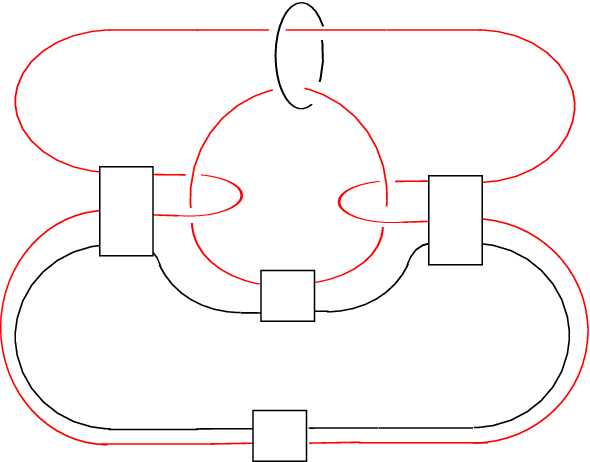
2pt
\pinlabel at 105 433
\pinlabel at 105 387
\endlabellist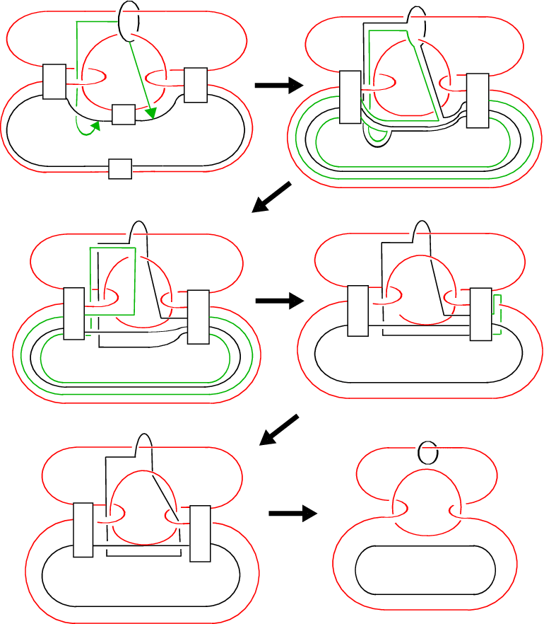
This construction was derived from the dual construction in [Go1], showing that the relevant homotopy balls are standard by introducing a canceling 2-handle/3-handle pair. While it was not easy to explicitly dualize the construction, in the end the two constructions appear rather similar. The construction in [Go1] also involves introducing a new link component and moving it around a torus. In that case, the new component was a 0-framed unknot, the attaching circle of the new 2-handle. Akbulut’s recent proof [Ak] that infinitely many Cappell-Shaneson homotopy 4-spheres are standard again relies on such a trick. In each case, the key seems to be an embedded torus with trivial normal bundle, to which a 2-handle is attached with framing , forming a fishtail neighborhood. This neighborhood has self-diffeomorphisms that can undo certain cut-and-paste operations on the 4-manifold, as we implicitly saw in the case of Proposition 10.1 with an embedding. While this procedure has been known in a different context for at least three decades, underlying the proof that simply connected elliptic surfaces with fixed are determined by their multiplicities, it still appears to be underused. In fact, one can obtain a simpler and more general proof that many Cappell-Shaneson 4-spheres are standard by going back to their original definition and directly locating fishtail neighborhoods [Go2].
References
- [Ak] S. Akbulut, Cappell-Shaneson homotopy spheres are standard, Annals of Mathematics (2) 171 (2010) 2171-2175.
- [CG] A. Casson and C. McA. Gordon, Reducing Heegaard splittings, Topology and its applications, 27 (1987) 275–283.
- [CL] T. Cochran, J. Levine, Homology boundary links and the Andrews-Curtis conjecture, Topology 30 (1991) 231–239.
- [Fr] M. Freedman, The topology of four-dimensional manifolds. J. Differential Geom. , 17 (1982) 357–453.
- [FGMW] M. Freedman, R. Gompf, S. Morrison, K. Walker, Man and machine thinking about the smooth -dimensional Poincaré conjecture, arXiv:0906.5177, to appear in Quantum Topology.
- [Ga1] D. Gabai, Foliations and the topology of -manifolds. II. J. Differential Geom. 26 (1987) 461–478.
- [Ga2] D. Gabai, Foliations and the topology of -manifolds. III, J. Differential Geom. 26 (1987) 479–536.
- [Ga3] D. Gabai, Surgery on knots in solid tori Topology 28 (1989) 1-6.
- [Ge] S. Gersten, On Rapaport’s example in presentations of the trivial group, preprint c. 1987.
- [Go1] R. Gompf, Killing the Akbulut-Kirby -sphere, with relevance to the Andrews-Curtis and Schoenflies problems Topology 30 (1991), 97–115.
- [Go2] R. Gompf, More Cappell-Shaneson spheres are standard, arXiv:0908.1914, to appear in Algebraic and Geometric Topology.
- [GS] R. Gompf and A. Stipsicz, -Manifolds and Kirby Calculus, Graduate Studies in Mathematics 20 American Mathematical Society, Providence, RI, 1999.
- [Hi] J. Hillman, Alexander ideals of links, Lecture Notes in Mathematics 895. Springer-Verlag, Berlin-New York, 1981.
- [Ki1] R Kirby, A calculus for framed links in Invent. Math. 45 (1978) 35–56.
- [Ki2] R Kirby, Problems in Low-Dimensional Topology, in Geometric Topology, Edited by H. Kazez, AMS/IP Vol. 2, International Press, 1997.
- [KM] R Kirby and P. Melvin, Slice knots and property R. Invent. Math (1978) 57–59.
- [LP] F Laudenbach and V Poénaru, A note on -dimensional handlebodies, Bull. Soc. Math. France 100 (1972) 337–344.
- [Ro] D. Rolfsen, Knots and Links, Mathematics Lecture Series, 7. Publish or Perish, Inc., Berkeley, Calif., 1976.
- [ST] M. Scharlemann, A. Thompson, Surgery on knots in surface I, Algebraic and Geometric Topology 9 (2009) 1825–1835