Fractal behind smart shopping
Abstract
The ‘minimal’ payment—a payment method which minimizes the number of coins in a purse—is presented. We focus on a time series of change given back to a shopper repeating the minimal payment. The delay plot shows visually that the set of successive change possesses a fine structure similar to the Sierpinski gasket. We also estimate effectivity of the minimal-payment method by means of the average number of coins in a purse, and conclude that the minimal-payment strategy is the best to reduce the number of coins in a purse. Moreover, we compare our results to the rule-60 cellular automaton and the Pascal-Sierpinski gaskets, which are known as generators of the discrete Sierpinski gasket.
1 Introduction
An English proverb says that “a heavy purse makes a light heart”, but we do not welcome a literal heavy purse full of coins. By repeated payments in everyday shopping, the number of coins in the shopper’s purse constantly increases or decreases, and sometimes the purse gets full of coins. A purse with a lot of coins is uneconomic because it becomes heavy and bulky, and even worse, the shopper has a lot of trouble in picking out coins from the purse. Electronic money[1] is hoped to eliminate such trouble, but it has not become a substitute for real cash so far because of technical, economical, and legal issues.
Some mathematical problems treat of coins. A famous one is known as the change-making problem[2]: how can a given amount of money be made with the least number of coins of given denominations? This problem is a variation of the knapsack problem[3], and it is known to be NP-hard[4]. The greedy algorithm[5] gives a solution in some limited cases, and other heuristic algorithms have been also proposed[6, 7, 8]. The optimality or efficiency of a monetary system itself has been also evaluated[9, 10, 11], and the Frobenius coin problem[12, 13, 14] asks what is the largest amount of money that cannot be obtained using only coins of specified denominations. We note that such problems are for retailers (how to make change) or for governments (what currency system is preferable); consumers are not considered. To prevent the swelling of a purse, which is a problem for consumers, we propose a method to minimize the number of coins in the purse through the payment. We also show that this method accompanies a remarkable mathematical structure like fractals.
2 What is the minimal payment?
We define the ‘minimal payment’ as follows. (i) A retailer keeps all kinds of coins sufficiently, and gives back change with the least number of coins. Namely, the retailer never gives 10-cent change by ten 1-cent coins or two 5-cent coins. (ii) The shopper pays with a combination of coins that minimizes the number of coins in the purse after the payment. (iii) The coins paid by the shopper and the ones given back to the shopper do not include common coins.
Let us play with a simple example. Imagine a nation where the coins are issued in , , and denominations (‘’ is the currency sign of this nation, and we also use this symbol as the generic currency sign in this paper, instead of the formal symbol ‘¤’), and a shopper in this nation has each of , , and coins in the purse, and is buying an item of . We compare two ways of payment. (1) If the shopper pays with one -coin alone, then the change is , hence three coins (one - and two -coins) are left in the purse. (2) If the shopper pays with one - and one -coins, then the change is (paid with one -coin), hence two -coins are left after the payment. Other payment patterns do not meet the condition (iii). Therefore, the minimal payment in this case is that the shopper pays with one - and one -coins and receives one -coin in change (see Fig. 1). The important fact is that the number of coins left in the shopper’s purse can vary according to the combination of coins in the payment.
Next we present the efficient calculation method of the minimal payment. Let us consider again the currency ‘’. The notation represents the content of the shopper’s purse, where , , and are respectively the number of , , and coins. In the above example, the coins before the payment are written as (see also Fig. 1). By using this vector-like notation, the total amount of money in the purse can be expressed as the scalar product: . In this sense, we identify a vector with the total amount, and simply express as . Returning to the above example, () is left in the purse after the purchase of an item of . Through the transition from (before the payment) to (after the payment), one - and one -coins are gone and one -coin is gained, which correspons to the minimal payment process (Fig. 1). We note that this calculation procedure for the minimal payment is far more efficient than the ‘full search’, and it can be applied straightforwardly to general currencies.
3 Fractality of successive minimal-payment processes
Here we show the mathematical structure of successive minimal-payment processes. We set the following four assumptions. (i) The shopper and the retailer iterate the minimal payment. (ii) Prices are generated randomly and independently in each payment, and we used a uniform random number in the numerical calculations. (iii) In order for the shopper not to lack money, we assume that the shopper has sufficiently large number of banknotes, and that the shopper can use banknotes if needed. (iv) Every coin is a multiple of the immediately smaller coin, and the smallest banknote is a multiple of the largest coin. We call (iv) the ‘multiplicable condition.’ For example, the Japanese yen (1000 yen bill; 500, 100, 50, 10, 5, 1 yen coins), the Korean won (1000 won bill; 500, 100, 50, 10, 5, 1 won coins), and the Swedish krona (20 krona bill; 10, 5, 1 krona, 50 öre (= 0.5 krona) coins) are multiplicable. However, the majority of currencies in the world is partially not multiplicable; in the US dollar (1 dollar (= 100 cent) bill; 50, 25, 10, 5, and 1 cent coins), 25 is not a multiple of 10.
For the analysis of successive change in the minimal payment, we employ the delay plot. For a given time series , the delay plot is defined as a planar point set . The delay plot is a useful tool for visualizing the correlation of adjoining pairs of the time series. In chaos theory[15] and nonlinear time series analysis[16], the delay plot is used for the reconstruction of an attractor from a series of experimental data. In general, a delay plot generated from a deterministic system forms an organized structure, whereas a plot from a stochastic noisy system forms an indistinct distribution.
Figure 2 illustrates the delay plot of a series of change generated by computer simulation of the minimal payment. In the simulation, we adopted the Japanese yen as the currency system (which holds the multiplicable condition), and iterated payment processes times. The whole structure is similar to the celebrated fractal object ‘Sierpinski gasket’[17].
In order to explain the mechanism of this quasi-fractal structure, let us go back once again to the model currency ‘’, where , , and coins are issued. We additionally imagine that the smallest banknote is denomination. Note that this currency is multiplicable. represents the coins in the shopper’s purse after the -th payment, and we set the initial condition . We also denote by the change given back in the -th payment. Since the prices are randomly generated, and are random variables. If ( coins in the purse increases), the -th change includes pieces of coin. Otherwise, if , the -th change includes no coins. Hence we can simply express as . The sum of the number of coins in -th and -th change is then calculated as
| (1) |
where we use the formula in a max-plus algebra[19]: . By the definition of the minimal payment and above algorithm, we can derive for any , where ‘1’ at the right hand side is given by the ratio of two denominations as . Therefore, the four arguments of ‘’ in Eq. (1) are all equal to or less than constantly, and we obtain as a result. Similarly, we can derive the relations and for and respectively. These relations signify that successive change and are correlated.
By the above calculation, the points of the delay plot are confined within the lattice points satisfying the conditions
| (2) |
As in Fig. 3, the effect of including smaller coins progressively generates a nested pattern (smaller coins contribute to higher resolution). In each iterative step, the blocks (the squares with bold contours) are replaced with smaller blocks aligned in a step-shape (or an L-shape), and finally the structure of the delay plot has a fine structure as in the Sierpinski gasket. Note that the side lengths, 12 (the length of the ‘whole’ block), 6, 2, and 1, of blocks in the iterative steps are identical with the denominations , , , and . This scenario of ‘successive replacement’ universally works on general multiplicable currency systems. In particular, if the denominations of coins grow geometrically (i.e., , , , ), the delay plot possesses (discrete) self-similarity, and its fractal dimension is given by
| (3) |
This expression also appears in a study of Pascal’s triangle[18]; we discuss delay plots and Pascal’s triangle in more detail in Section 6. The multiplicable condition is necessary for the realization of a regular shape of the delay plot. For example, the delay plot of the US dollar exhibits a relatively disordered structure, reflecting the breaking of the multiplicable condition between 25 and 10 cent coins (Fig. 4).
4 Effectivity of the minimal payment
Here we comment on the effectivity of the minimal-payment method, measured by the average number of coins in the shopper’s purse. We estimated this average numerically. In this calculation, we adopted the US dollar as the currency, and iterated the minimal payment times. The results are summarized in Fig. 5. Figure 5 (a) shows the fluctuation of the number of coins in the purse of the first 1000 steps, and Fig. 5 (b) is the numerically-generated probability distribution of the number of coins in the purse. By taking the mean value of Fig. 5 (b), the number of coins in the purse is 4.20 pieces on average. Furthermore, the maximum number of coins in Fig. 5 (b) is eight. Thus, by using the minimal-payment strategy, we can constantly keep the coins in a purse 8 pieces or less.
We can also calculate this average more rigorously. Since the prices are distributed randomly and independently in our numerical model, a probability of the amount of money in the purse becomes uniform. Figure 6 illustrates how many coins are needed to represent each amount of money, and the average number of coins is exactly 4.2 pieces by taking the mean value. Note that the two distributions in Fig. 5 (b) and Fig. 6 (b) are so alike.
The average number can be calculated easily for a multiplicable currency. For the model currency ‘’ ( bill; , , and coins), the set of possible amounts of money in a purse is
| (4) |
For the same reason as above, each amount of money listed in Eq. (4) emerges with a uniform probability. In Eq. (4), the possible numbers of coins are either 0 or 1, which appear six times each. Thus, the average number of coins is 0.5, which is also given by . The same estimation is valid for the numbers of and coins. Therefore, the average number of coins in a purse is
We can straightforwardly apply this formula to any multiplicable currencies. For example, the average number of the Japanese yen (1000 yen bill; 500, 100, 50, 10, 5, and 1 yen coins) is both 7.5 pieces.
Conversely, we note that this average number can be regarded as the lower bound, that is, we cannot keep down the average number of coins below this lower bound, no matter what payment strategy is used. This is the ‘minimality’ of the presented payment method.
5 Relevance to the rule-60 cellular automaton
In the present section, let us consider the denominations of coins grow with a binary scale, that is, the coins are , , , , , , and the smallest banknote is . As in Section 3, let denote the number of coins in -th change, and the condition holds for any and . The corresponding delay plot is obtained by solving
| (5) |
In other words, and never take place at the same time. The delay plot forms the discrete Sierpinski gasket (Fig. 7).
The discrete Sierpinski gasket appears in various systems in mathematics and physics, ranging from an analysis of the Tower of Hanoi[20] to pulse dynamics in a reaction-diffusion system[21] and a model of fracture[22]. As a typical example, we focus on the rule-60 cellular automaton in this section.
A cellular automaton (CA)[23] is a discrete dynamical system on cells aligned linearly. The possible state of each cell is either ‘0’ or ‘1’, and the evolution of states generally depends on their own state and the states of their neighbors. In particular, the rule-60 CA can generate the discrete Sierpinski gasket, which is driven by the following rule. (i) If a cell and its left neighbor are in the same state, the next state of the cell is 0. (ii) Otherwise (i.e., the states of the two cells are different), the next state is 1. This evolution rule is schematically shown in Fig. 8 (a). We denote by the state of -th cell at time . Then, the evolution of the state is simply expressed as , where is an exclusive-or operation defined as and . A resultant pattern is depicted in Fig. 8 (b), where the initial condition is that one cell is ‘1’ and the others are ‘0’. The evolution rules of other cellular automata, such as rule-90, 22, 154 and 102, can be expressed by , and they also generate discrete Sierpinski gaskets.
Similarity between a delay plot of binary coins (Fig. 7) and the evolution pattern of the rule-60 CA (Fig. 8 (b)) is obvious. We discuss this similarity more in detail. Figure 9 shows iterative steps for solving Eq. (5). As a condition for a smaller coin is considered, the blocks in each step are subdivided according to the following rule:
| (6) |
As shown in Fig. 10 (a), this subdivision preserves the exclusive-or structure of the rule-60 CA. Moreover, a spatio-temporal pattern after the subdivision is similar to the one before the subdivision, that is, the subdivision works on the rule-60 CA as a spatio-temporal scale transformation. Both the unit lengths of space and time are halved by subdivision (see Fig. 10 (b)). Therefore, we conclude that the key to similarity between the delay plot of a binary currency and the rule-60 CA is compatibility of the rule (6) of subdivision and the exclusive-or relation.
6 Comparison with the Pascal-Sierpinski gaskets
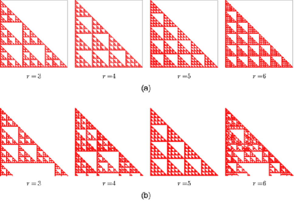
Pascal’s triangle (Fig. 11 (a)) also generates a discrete Sierpinski gasket by coloring the odd numbers (Fig. 11 (b))[24]. Clearly, Fig. 11 (b) is essentially the same as Fig. 7 and Fig. 8 (b). In fact, the coloring rule is reduced to the exclusive-or operation[25]. As a generalization, the Pascal-Sierpinski gasket[26] of modulo is obtained by coloring the elements not divisible by . In this section, we compare the Pascal-Sierpinski gasket of modulo and the delay plot of the coins , , , .
In Fig. 12 (a), we show the delay plots corresponding to , and 6. The shapes of them are quite similar to the Sierpinski gasket. In contrast, the Pascal-Sierpinski gaskets are more complicated (Fig. 12 (b)). In the case of and 5, the Pascal-Sierpinski gaskets are similar to the corresponding delay plots. However, the Pascal-Sierpinski gaskets of modulo and 6 exhibit disordered structure, and they looks different from the delay plots of such . According to the theory[27] of the Pascal-Sierpinski gasket, the Pascal-Sierpinski gasket possess the same structure as the corresponding delay plot if is a prime number; however, the pattern is more complicated if is a composite number.
7 Discussion
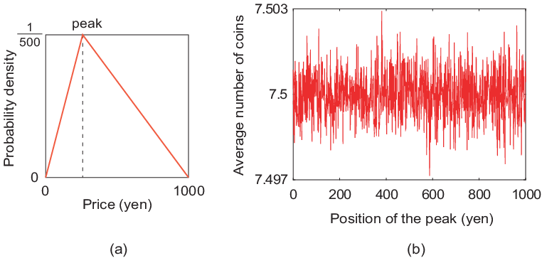
In the numerical simulations of the minimal payment in this paper, we assume that the prices are distributed randomly, independently, and uniformly. Randomness and independentness are reasonable for real payment, but uniformness is a debatable point. In fact, the range of prices depends on each person’s life style or consumption behavior. We simply model this non-uniform occurrence of prices by using a triangular random number. In this numerical calculation, the Japanese yen (1000 yen bill; 500, 100, 50, 10, 5, and 1 yen coins) was used as a currency, and we iterated the minimal-payment processes times. The prices are generated by a triangular random number on the interval , and the position of the peak of the triangle is a control parameter (Fig. 13 (a)). The result is shown in Fig. 13 (b). The average numbers of coins in the purse are within , which is irrespective of the position of the peak of triangle. Thus, the average number of coins in a purse is still 7.5 pieces also in this more realistic case. We expect that the average number of coins in a purse remains constant over a wide class of probability distributions of prices.
The term ‘fractal time series’ or ‘temporal fractal’ conventionally means that a time series has scale-invariance or power-law spectrum[30, 31, 32]. On the other hand, the time series of change in successive minimal payment is another type of ‘fractal time series’ in the sense that its delay plot exhibits self-similarity. We note that the power spectrum of a time series of change does not exhibit power law.
The vector-like notation is a generalization of the binary (or -adic) expansion, which is an essential tool in computer science[33, 34]. A cellular automaton was invented as a prototype of digital computing. Namely, our analysis originates from analogue payment, and leads to digital fractals. In the analysis, we assume that a retailer gives back change with the least number of coins. However, real retailers may not give change with the least number of coins because they may run out of coins of certain denominations, or may feel that finding the least number is troublesome. This causes the increase of the number of coins in a purse. Thus, realization of the ‘minimal’ requires the retailers’ cooperation, but we emphasize that we can avoid immoderate swelling of a purse at least if we pay attention to our payment styles.
8 Conclusion
We demonstrated that a payment method affects the number of coins left in a purse, and showed how to minimize the number of coins in a purse after a payment. We called this method the ‘minimal payment’. By using the delay plot, a time series of change under successive minimal-payment processes a fine structure like the Sierpinski gasket. The mechanism of this fine structure is reduced to a coupled inequalities as in Eqs. (2) and (5). We also compared delay plots and the rule-60 cellular automaton and the Pascal-Sierpinski gasket.
Acknowledgments
We are very greatful to Dr. Mitsugu Matsushita and Dr. Hiroto Kuninaka for their beneficial comments. One of the authors (K.Y.) is a Research Fellow of the Japan Society for the Promotion of Science.


References
- [1] A. Furche and G. Wrightson, Computer Money: A Systematic Overview of Electronic Payment Systems, Morgan Kaufmann, Massachusetts, 1996.
- [2] S.K. Chang and A. Gill, Journal of the ACM, 17 (1970) 113-122.
- [3] S. Martello and P. Toth, Knapsack Problems: Algorithms and Computer Implementations, John Wiley and Sons, Chichester, 1990.
- [4] J. Hromkovič, Algorithmics for Hard Problems, Springer, Berlin, 2001.
- [5] M.J. Magazine, G.L. Nemhauser, and L.E. Trotter, Oper. Res., 23 (1975) 207-217.
- [6] J.W. Wright, J. ACM, 22 (1975) 125-128.
- [7] D. Pearson, Oper. Res. Lett., 33 (2005) 231-234.
- [8] S. Böcker and Z. Lipták, Algorithmica, 48 (2007) 413-432.
- [9] L.G. Telser, Economics Lett., 49 (1995) 425-427.
- [10] A.E. Tschoegl, J. Money, Credit and Banking, 29 (1997) 546-554.
- [11] J. Shallit, The Mathematical Intelligencer, 25 (2003) 20-23.
- [12] A. Nijenhuis and H.S. Wilf, J. Number Th., 4 (1972) 98-106.
- [13] R. Kannan, Combinatorica, 12 (1992) 161-177.
- [14] M. Beck and S. Robins, Computing the Continuous Discretely: Integer-pint Enumeration in Polyhedra, Springer, Berlin, 2007.
- [15] K.T. Alligood, T.D. Sauer, and J.A. Yorke, Chaos: an Introduction to Dynamical Systems, Springer, New York, 1997.
- [16] H. Kantz and T. Schreiber, Nonlinear Time Series Analysis, Cambridge Univ. Press, 1997.
- [17] W. Sierpiński, Compt. Rendus. Acad. Sci. Paris, 160 (1915) 302-305.
- [18] T.W. Gamelin and M.A. Mnatsakanian, Publ. Mat., 49 (2005) 329-349.
- [19] F. Baccelli, G. Cohen, G.J. Olsder, and J.-P. Quadrat, Synchronization and Linearity, John Wiley and Sons, Chichester, 1992.
- [20] A.M. Hinz, Amer. Math. Monthly, 99 (1992) 538-544.
- [21] Y. Hayase and T. Ohta, Phys. Rev. Lett., 81 (1998) 1726-1729.
- [22] M. Matsushita, J. Phys. Soc. Jpn., 54 (1985) 857-860.
- [23] S. Wolfram, Rev. Mod. Phys., 55 (1983) 601-644.
- [24] S. Wolfram, Amer. Math. Monthly, 91 (1984) 566-571.
- [25] K. Culik and S. Dube, Complex Systems, 3 (1989) 253-267.
- [26] N.S. Holter, A. Lakhtakia, V.K. Varadan, and R. Messier, J. Phys. A: Math. Gen., 19 (1986) 1753-1759.
- [27] M. Frame and N. Neger, Computers & Graphics, 34 (2010) 158-166.
- [28] H.-O. Peitgen, H. Jürgens, D. Saupe, E. Maletsky, and T. Perciante, Fractals for the Classroom: Strategic Activities, vol. 3, Springer, New York, 1999.
- [29] H.-O. Peitgen, H. Jr̈gens, and D. Saupe, Chaos and Fractals: New Frontiers of Science, Springer, New York, 1992.
- [30] T. Higuchi, Physica D, 31 (1988) 277-283.
- [31] Y. Yamamoto and R.H. Hughson, Physica D, 68 (1993) 250-264.
- [32] D. C. Caccia, D. Percival, M.J. Cannon, G. Raymond, and J.B. Bassinghtwaighte, Physica A, 246 (1997) 609-632.
- [33] D.E. Knuth, The Art of Computer Programming, Addison-Wesley, Reading, 1981.
- [34] M.W. Baldoni, C. Ciliberto, and G.M.P. Cattaneo, Elementary Number Thory, Cryptography and Codes, Springer, Berlin, 2009.