Scalable Approach to Uncertainty Quantification and Robust Design of Interconnected Dynamical Systems

Andrzej Banaszuk Vladimir A. Fonoberov Thomas A. Frewen^* Marin Kobilarov George Mathew Igor Mezic Alessandro Pinto^§ Tuhin Sahai^* Harshad Sane^* Alberto Speranzon^* Amit Surana^* ^†^†thanks: United Technologies Research Center, East Hartford, CT 06118, USA^†^†thanks: AIMdyn Inc., Santa Barbara, CA 93101, USA^†^†thanks: California Institute of Technology, Pasadena, CA 91125, USA^†^†thanks: United Technologies Research Center Inc, Berkeley, CA 94705, USA^†^†thanks: University of California, Santa Barbara, CA 93106,USA

Abstract

Development of robust dynamical systems and networks such as autonomous aircraft systems capable of accomplishing complex missions faces challenges due to the dynamically evolving uncertainties coming from model uncertainties, necessity to operate in a hostile cluttered urban environment, and the distributed and dynamic nature of the communication and computation resources. Model-based robust design is difficult because of the complexity of the hybrid dynamic models including continuous vehicle dynamics, the discrete models of computations and communications, and the size of the problem. We will overview recent advances in methodology and tools to model, analyze, and design robust autonomous aerospace systems operating in uncertain environment, with stress on efficient uncertainty quantification and robust design using the case studies of the mission including model-based target tracking and search, and trajectory planning in uncertain urban environment. To show that the methodology is generally applicable to uncertain dynamical systems, we will also show examples of application of the new methods to efficient uncertainty quantification of energy usage in buildings, and stability assessment of interconnected power networks.

Keywords
Aerospace Systems; Graph Decomposition; Model Based Design; Motion Planning; Uncertainty

1 Introduction

In this paper we discuss methodology and tools enabling model-based design of complex interconnected dynamical systems that would operate as desired in the presence of uncertainty in models and environment. A particular challenge problem we are going to consider is design of unmanned aerospace systems that can conduct complex missions in a safe, predictable, and robust manner. Model-based robust design is difficult for such systems because of the environmental and modeling uncertainties, and the overall system complexity. Dynamically evolving uncertainties arise from model uncertainties, necessity to operate in a adversarial cluttered urban environment, and the distributed and dynamic nature of the communication and computational resources. Complexity results from the hybrid dynamic models including continuous vehicle dynamics, the discrete models of computations and communications, and the size of the problem. We overview recent advances in methodology and tools for managing uncertainty and complexity in such interconnected dynamical systems. We illustrate this methodology for modeling, analysis and robust design of autonomous aerospace systems using case studies, which include low level autonomous flight in urban environment and model-based target tracking and search. To show the generality of our approach, we also include examples of efficient uncertainty quantification of energy usage in buildings, and stability assessment of interconnected power networks.

The objective of Robust Uncertainty Management (RUM) project [5] was to develop methodology and tools for quantifying uncertainty in ways that are orders of magnitude faster than Monte Carlo with near-linear scaling in the system size, and demonstrate them in molecular dynamics and UAV search challenge problems. Several Uncertainty Quantification (UQ) methods including Polynomial Chaos (PC), and new Stochastic Response Surface, and Dynamic Sampling methods were applied to calculate the mean and variance of the phase transition temperature in molecular dynamics calculations with 10000 atoms 2000 times faster than using Monte Carlo sampling. The new search strategies described in [5] achieved 2x reduction in the median search time compared with a standard lawnmower approach in a challenge problem including 50 simulated UAVs searching for a stationary target in a complex terrain using noisy sensors with uncertain footprint. One method used a trajectory planner based on the use of a library of pre-computed elementary UAV trajectory segments that individually satisfy the vehicle dynamics and can be interlocked to produce large scale roadmaps. In this paper we provide an overview of selected methods and tools for Uncertainty Management and Stochastic Design Methodology that started within the RUM project and were continued under the Autonomous and Intelligent Systems initiative at United Technologies Research Center (UTRC), including strong collaboration with researchers at UCSB, Caltech, and Aimdyn, Inc.

The key idea that enables scalable computations in interconnected dynamic networks presented in Section 2 of this paper is that of decomposing large networks of dynamical components into weakly connected subnetworks using spectral properties of a graph Laplacian constructed from a Jacobian matrix of the underlying set of ODEs describing the dynamic network. This graph decomposition method for dynamic networks was first introduced in [70]. The decomposition allows to parallelize the problem of solving large ODEs using the method called Waveform Relaxation [72]. Iterations across weak connections yield a provably convergent method under the assumption that underlying set of ODEs satisfies the Lipshitz condition. A new efficient and easily parallelizable method of obtaining spectral decomposition applicable to large dynamic networks has been introduced in [59] and is described in Section 2. Rather than relying on random walk methods used in state of the art methods for distributed computations of spectral properties of matrices, the method relies on using the Graph Laplacian corresponding to the dynamic network of interest to define and solve a wave equation.

In Section 3 we show how the graph decomposition introduced in Section 2 can be generalized to scalable Uncertainty Quantification using a method called Probabilistic Waveform Relaxation introduced in [67]. Once the dynamic network is decomposed into weakly connected subnetworks, efficient methods for Uncertainty Quantification are applied to subnetworks in an iterative manner. The method is called Probabilistic Waveform Relaxation and is amenable to parallel computations. We demonstrate the method on examples from energy flow in buildings and power networks.

In Section 4 we address another aspect of Uncertainty Management: design of search and tracking algorithms for unmanned aerospace systems that allow to reduce the uncertainty of location of stationary or mobile targets. For search and tracking applications, it is important to design uniform coverage dynamics for mobile sensors. A uniform coverage control algorithm would ensure that the amount of time spent by the sensors observing a neighborhood is proportional to the probability of finding a target in the neighborhood. For the search of a stationary target, the uncertainty in the position of the target can be specified in terms of a fixed probability distribution. The Spectral Multiscale Coverage algorithm proposed in ([45] and [46]), makes the sensors move so that points on the sensor trajectories uniformly sample this stationary probability distribution. Uniform coverage dynamics coupled with sensor observations helps to reduce the uncertainty in the position of the target. In [27], it has been demonstrated that in the presence of various uncertainties, uniform coverage based search strategies outperform lawnmower-type search strategies. In a recent paper [48] we extended the SMC algorithm to the case of moving targets.

While in Section 4 we consider a simplistic model of a mobile sensor and no obstacles, in Section 5 we consider a considerably more difficult problem of optimizing a motion of a vehicle described by a realistic model of motion in an obstacle-rich environment. The vehicle is subject to constraints arising from underactuated dynamics, actuator bounds, and obstacles in the environment. We assume that the vehicle is equipped with a sensor measuring the relative positions of obstacles. The problem has no closed-form solution since both the dynamics and constraints are nonlinear. Gradient-based optimization is not suitable unless a good starting guess is chosen since the obstacles impose many local minima. In this paper we also employ a graph-based search but unlike in standard discrete search, the nodes of the tree are sampled from the original continuous space and the edges correspond to trajectories satisfying any given dynamics and general constraints. Our approach is based on a recent methodology under active development in the robotics community known as sampling-based motion planning which includes the rapidly-exploring random tree (RRT) [38] and the probabilistic roadmap (PRM) [9]. In our framework samples are connected through sequences of locally optimized precomputed motion primitives. The two main advantages of the approach is that the locally optimal motion primitives used are computed offline and that standard graph search methods can be used for finding global solutions efficiently. Note that even if the model of the vehicle is assumed deterministic and perfectly known, the introduction of sampling-based motion planning introduces uncertainty in the trajectory planing process. In particular, one can only characterize the probability of computing a feasible path as a function of the number of samples.

In Section 6 we show how the techniques presented in this paper are organized into a design process. We shows how analysis and synthesis tools can be effectively used in a design flow that is based on the notion of abstraction levels. While Section 2 and 3 present decomposition techniques that apply to one particular abstraction level, the methodology in Section 6 shows how a design problem is vertically decomposed into refinement steps. For example, search and tracking algorithms can rely on an abstraction of the low level path planner. In this section we also discuss the challenges in the integration and deployment of tools to serve development of industrial applications. We conclude the section by showing our efforts in this direction.

2 Bottom up graph decomposition

In recent years, there has been an exponential increase of interest in large interconnected systems, such as sensors networks, thermal networks, social networks, internet, biochemical networks, power networks, communication networks etc. These systems are characterized by complex behavior arising because of interacting subsystems. Often these interactions are weak which can be exploited to simplify and accelerate the simulation, analysis and design of such systems by suitably decomposing them. To facilitate this decomposition it is convenient to model such networked systems by a graph of interacting subsystems. Consequently, graph theoretic methods have been recently applied and extended to study these systems. To illustrate this idea, consider a large interconnected system described by a system of differential equation

	$\displaystyle\dot{x_{1}}$	$\displaystyle=$	$\displaystyle f_{1}(\mathbf{x},\mathbf{\xi}_{1},t),$
	$\displaystyle\dot{x_{n}}$	$\displaystyle=$	$\displaystyle f_{n}(\mathbf{x},\mathbf{\xi}_{n},t),$		(1)

where, $\mathbf{f}=(f_{1},f_{2},\cdots,f_{n})\in\mathbb{R}^{n}$ is a smooth vector field, $\mathbf{x}=(x_{1},x_{2},\cdots,x_{n})\in\mathbb{R}^{n}$ are state variables, $\mathbf{\xi}_{i}\in R^{p_{i}}$ is vector of (possibly uncertain) parameters affecting the $i-$ th system. Let $\mathbf{\xi}=(\mathbf{\xi}_{1}^{T},\cdots,\mathbf{\xi}_{n}^{T})^{T}\in\mathbb{R}^{p}$ be the $p=\sum_{i=1}^{n}p_{i}$ dimensional vector of parameters affecting the complete system. The solution to initial value problem $\mathbf{x}(t_{0})=\mathbf{x}_{0}$ will be denoted by $\mathbf{x}(t;\mathbf{\xi})$ , where for brevity we have suppressed the dependence of solution on initial time $t_{0}$ and initial condition $\mathbf{x}_{0}$ . Given the set of state variables $x_{1},\cdots,x_{n}$ and some notion of dependence ${\mathbf{W}}_{ij}\geq 0,i=1,\cdots,n,j=1,\cdots,n$ between pairs of state variables, a graph can be constructed. The vertices in this graph represent the states variables $x_{i}$ and two vertices are connected with an edge of weight ${\mathbf{W}}_{ij}$ . In order to quantify coupling strength ${\mathbf{W}}_{ij}$ between nodes or state variables, one could use for example [49]

{\mathbf{W}}_{ij}=\frac{1}{2}[|\overline{J}_{ij}|+|\overline{J}_{ji}|],

(2)

where, $\overline{J}=[\frac{1}{T_{s}}\int_{t_{0}}^{t_{0}+T_{s}}J_{ij}(\mathbf{x}(t;\mathbf{\xi}_{m}),\mathbf{\xi}_{m},t)dt]$ , is time average of the Jacobian,

J(\mathbf{x},\mathbf{\xi},t)=\left[\frac{\partial f_{i}(\mathbf{x}(t;\mathbf{\xi}),\mathbf{\xi},t)}{\partial x_{j}}\right],

(3)

computed along the solution $\mathbf{x}(t;\mathbf{\xi})$ of the system (7) for nominal value of parameters $\mathbf{\xi}_{m}$ . The decomposition or clustering problem can now be formulated as follows: find a partition of the graph such that the edges between different components have a very low weight and the edges within a component have high weights. The main tool for accomplishing such a decomposition is the graph Laplacian. In particular, spectral properties of the Laplacian matrix $L$ associated to such graphs provide very useful information for the analysis as well as the design of interconnected systems. The computation of eigenvectors of the graph Laplacian $L$ is the cornerstone of spectral graph theory [10, 71], and it is well known that the sign of the second (and successive eigenvectors) can be used to cluster graphs [15, 16].

Let $\mathcal{G}=(V,E)$ be a graph with vertex set $V=\{1,\dots,N\}$ and edge set $E\subseteq V\times V$ , where a weight ${\mathbf{W}}_{ij}\in\mathds{R}$ is associated with each edge $(i,j)\in E$ , and ${\mathbf{W}}\in\mathds{R}^{N\times N}$ is the weighted adjacency matrix of $\mathcal{G}$ . We assume that ${\mathbf{W}}_{ij}=0$ if and only if $(i,j)\notin E$ . The (normalized) graph Laplacian is defined as,

\displaystyle{\mathbf{L}}_{ij}=\begin{cases}1&\mbox{if}\>i=j\\ -{\mathbf{W}}_{ij}/\sum_{\ell=1}^{N}{\mathbf{W}}_{i\ell}&\mbox{if}\>(i,j)\in E\\ 0&\mbox{otherwise}\,.\end{cases}

In this work we only consider undirected graphs. The smallest eigenvalue of the Laplacian matrix is $\lambda_{1}=0$ , with an associated eigenvector ${\mathbf{v}}^{(1)}=\mathbf{1}=\left[1,1,\dots,1\right]^{T}$ . Eigenvalues of ${\mathbf{L}}$ can be ordered as, $0=\lambda_{1}\leq\lambda_{2}\leq\lambda_{3}\leq\cdots\leq\lambda_{N}$ with associated eigenvectors $\mathbf{1},{\mathbf{v}}^{(2)},{\mathbf{v}}^{(3)}\cdots{\mathbf{v}}^{(N)}$ [71]. It is well known that the multiplicity of $\lambda_{1}$ is the number of connected components in the graph [50]. We assume in the following that $\lambda_{1}<\lambda_{2}$ (the graph does not have trivial clusters). We also assume that there exists unique cuts that divide the graph into $k$ clusters. In other words, we assume that there exist $k$ distinct eigenvalues [69].

Given the Laplacian matrix ${\mathbf{L}}$ , associated with a graph $\mathcal{G}=(V,E)$ , spectral clustering divides $\mathcal{G}$ into two clusters by computing the sign of the $N$ elements of the second eigenvector ${\mathbf{v}}^{(2)}$ , or Fiedler vector [16, 71].

As the clustering is decided by the eigenvectors/eigenvalues of the Laplacian matrix one can use standard matrix algorithms for such computation [23]. Since we are considering multi-agent systems, the execution of these standard algorithms is infeasible in decentralized settings. To address this issue, algorithms for distributed eigenvector computations have been proposed [32]. These algorithms, however, are also (like the algorithm in [63]) based on the slow process of performing random walks on graphs.

The slowest step in the distributed computation of eigenvectors is the simulation of a random walk on the graph. This procedure is equivalent to solving the discrete version of the heat equation on the graph. The connection between spectral clustering and the heat equation was also pointed out in [51, 52].

In a theme similar to M. Kac’s question “Can one hear the shape of a drum?” [30], we demonstrate that by simulating the wave equation over a graph, nodes can “hear” clusters of the graph Laplacian using only local information. Moreover, we demonstrate, both theoretically and on examples, that the wave equation based algorithm is orders of magnitude faster than random walk based approaches for graphs with large mixing times. The overall idea of the wave equation based approach is to simulate, in a distributed fashion, the propagation of a wave over a graph and capture the frequencies at which the graph “resonates”. In this paper we show that from such frequencies it is possible to exactly recover the eigenvectors of $L$ from which the clustering problem is solved. We also provide conditions the wave must satisfy in order to cluster a graph using the proposed method.

2.1 Wave Equation Based Clustering

Similar to the case of the heat equation, the solution of the wave equation

\frac{\partial^{2}u}{\partial t^{2}}=c^{2}\Delta u\,.

(4)

can be expanded in terms of the eigenvectors of the Laplacian. However, unlike the heat equation where the solution eventually converges to the first eigenvector of the Laplacian, in the wave equation all the eigenvectors remain eternally excited [14]. Here we use the discretized wave equation on graphs to develop a simple, yet powerful, eigenvector computation algorithm. The main steps of the algorithm are shown as Algorithm 2.1. Note that some properties of the wave equation on graphs have been studied in [20].

Algorithm 2.1 Wave equation based eigenvector computation algorithm for node

i

. At node

i

one computes the sign of the

i

-th component of the first

k

eigenvectors. The vector

{\mathbf{v}}^{(j)}_{i}

is the

i

-th component of the

j

-th eigenvector. The cluster number is obtained from interpreting the vector of

k

signs as a binary number.

{\bf u}_{i}(0)\leftarrow\texttt{Random}\>([0,1])

{\bf u}_{i}(-1)\leftarrow{\bf u}_{i}(0)

t\leftarrow 1

4: while

t<T_{max}

{\bf u}_{i}(t)\leftarrow 2{\bf u}_{i}(t-1)-{\bf u}_{i}(t-2)-

\qquad\qquad c^{2}\sum_{j\in\mathcal{N}(i)}{\mathbf{L}}_{ij}{\bf u}_{j}(t-1)

t\leftarrow t+1

7: end while

Y\leftarrow\texttt{FFT}\>(\left[{\bf u}_{i}(1),\dots\dots,{\bf u}_{i}(T_{max})\right])

9: for

j\in\{1,\dots,k\}

10:

\theta_{j}\leftarrow\texttt{FrequencyPeak}\>(Y,j)

11:

{\mathbf{v}}^{(j)}_{i}\leftarrow\texttt{Coefficient}(\theta_{j})

12: if

{\mathbf{v}}^{(j)}_{i}>0

then

13:

C_{j}\leftarrow 1

14: else

15:

C_{j}\leftarrow 0

16: end if

17: end for

18: ClusterNumber

\leftarrow\sum_{j=1}^{k}C_{j}2^{j-1}

Proposition 2.1.

The clusters of the graph $\mathcal{G}$ , as determined by the sign of the elements of Fiedler’s eigenvector (as well as higher order eigenvectors) of ${\mathbf{L}}$ , can be equivalently computed using the frequencies and coefficients obtained from the Fast Fourier Transform of $({\bf u}_{i}(1),\dots,{\bf u}_{i}(T))$ , for all $i$ . Here ${\bf u}_{i}$ is governed by the wave equation on the graph with initial condition ${\bf u}(-1)={\bf u}(0)$ .

Proposition 2.2.

The wave equation iteration (Step 5 in Algorithm 2.1) is stable on any graph if the speed of the wave satisfies the following inequality, $c\leq\sqrt{2}$ .

Proof of these propositions can be found in [59].

An important quantity related to the wave equation based algorithm is the time needed to compute the eigenvalues and eigenvectors components. The distributed eigenvector algorithm proposed in [32] converges at a rate of $O(\tau\log^{2}(N))$ , where $\tau$ is the mixing time of the Markov chain associated with the random walk on the graph. We derive a similar convergence bound for the wave equation based algorithm.

It is evident that one needs to resolve the lowest frequency to cluster the graph [59]. Let us assume that one needs to wait for $\eta$ cycles of the lowest frequency to resolve it successfully (i.e. the number of cycles needed for a peak to appear in the FFT)¹¹ 1 The constant $\eta$ is related to the FFT algorithm and independent of the graph. Typically 6-7 cycles of the lowest frequency are necessary to discriminate it.. The time needed to cluster the graph based on the wave equation is,

T=O\left(\frac{1}{\arccos(e^{-1/\tau})}\right)+O(N)\,.

(5)

For details of the derivation see [59].

Figure 1: Comparison of convergence between distributed algorithm [32] and proposed wave equation algorithm. Wave equation based algorithm has better scaling with

\tau

for graphs of any size (given by

N

). Of course the plots are upper bounds on the convergence speed, but they are anyway indicative.

2.2 Numerical Examples

To check the accuracy of our distributed wave equation based clustering algorithm, we demonstrate our approach on several examples.

2.2.1 Social Network

The first example is the Fortunato benchmark graph [36] with $1000$ nodes and $99084$ edges. Here the graph represents a social network with two communities (clusters) with $680$ and $320$ nodes respectively. Since these clusters are known apriori we can check the accuracy of our approach. We find that the wave equation based clustering computes the graph cut exactly. These clusters are shown in Fig. 2.

Refer to caption — Figure 2: A Fortunato community detection benchmark with $1000$ nodes and $99084$ edges. Wave equation based clustering computes the graph cut exactly.

2.2.2 Building Thermal Network

For energy consumption computation, a building can be represented in terms of a reduced order thermal network model [54],

\frac{dT}{dt}=A(t;\xi)T+B\left(\begin{array}[]{c}Q_{e}(t)\\ Q_{i}(t)\\ \end{array}\right)

(6)

where, $T\in R^{n}$ is a vector comprising of internal zone air temperatures, and internal and external wall temperatures; $A(t;\xi)$ is the time dependent matrix with $\xi$ being parameters, and $Q_{e}$ and $Q_{i}$ represent the solar radiation and occupant load. Figure 3a shows schematic of a building and key elements of a thermal network model. For the particular building considered, the network model is derived by lumping one of the building floors into 6 zones and comprises of $68$ state variables. This model admits a decomposition into $23$ subsystems, as revealed by the spectral graph approach (see figure 3c). This decomposition is consistent with three different time scales (associated with external and internal wall temperature, and internal zone temperatures) present in the system, as shown by the three bands in figure 3b.

2.3 Extensions

Current work includes the extension of the wave equation based algorithm for dynamic networks. This is clearly very important in situations where the weights on the edges of the graph are time varying. The authors are also extending these algorithms to cluster multi-attributed graphs (with multiple edges between any two nodes) and pursuing multi-scale versions of the wave-equation based clustering method. We are also developing methods which exploit the system decomposition to accelerate simulation and analysis of networked dynamical systems. On such application to uncertainty quantification is described in the next section.

3 Scalable Uncertainty Quantification

Uncertainty Quantification (UQ) methods provide means of calculating probability distribution of system outputs, given probability distribution of input parameters. Outputs of interest could include for example, latency in communication network, power quality and stability of power networks, and energy usage in thermal networks. The standard UQ methods such as Monte Carlo(MC) [17] either exhibit poor convergence rates or others such as Quasi Monte Carlo (QMC) [53][60], generalized Polynomial Chaos(gPC) [74] and the associated Probabilistic Collocation method (PCM) [73], suffer from the curse of dimensionality (in parameter space), and become practically infeasible when applied to network as a whole. Improving these techniques to alleviate the curse of dimensionality is an active area of current research, see [1] and references therein: notable methods include sparse-grid collocation method [22],[18] and ANOVA decomposition [61] for sensitivity analysis and dimensional reduction of the uncertain parametric space. However, none of such extensions exploits the underlying structure and dynamics of the networked systems which can often prove advantageous. For example, authors in [43, 21] used graph decomposition to facilitate stability and robustness analysis of large-scale interconnected dynamical systems. Mezic et al. [49] used graph decomposition in conjunction with Perron Frobenius operator theory to simplify the invariant measure computation and uncertainty quantification, for a particular class of networks. While these approaches exploit the underlying structure of the system, they do not take advantage of the weakly coupled dynamics of the subsystems.

3.1 Probabilistic Waveform Relaxation

We propose an iterative UQ approach that exploits the weak interactions among subsystems in a networked system to overcome the dimensionality curse associated with traditional UQ methods. This approach relies on integrating graph decomposition techniques and waveform relaxation schemes with probabilistic collocation and generalized polynomial chaos. Graph decomposition to identify weakly interacting subsystems was described in section 2. Waveform relaxation [72], a parallelizable iterative method, on the other hand, exploits this decomposition and evolves each subsystem forward in time independently but coupled with the other subsystems through their solutions from the previous iteration. At each waveform relaxation iteration we propose to apply PC at subsystem level and use gPC to propagate the uncertainty among the subsystems. Since UQ methods are applied to relatively simpler subsystems which typically involve a few parameters, this renders a scalable iterative approach to UQ in complex networks. We refer to this iterative UQ approach as probabilistic waveform relaxation (PWR).

We illustrate the proposed PWR framework through an example of parametric uncertainty in a simple system (7). The PWR framework also applies to DAE models and stochastic processes as will be described later. Consider the following system:

$\displaystyle\dot{x_{1}}$	$\displaystyle=$	$\displaystyle f_{1}(x_{1},x_{2},\xi_{1},t),$
$\displaystyle\dot{x_{2}}$	$\displaystyle=$	$\displaystyle f_{2}(x_{1},x_{2},x_{3},\xi_{2},t),$	(7)
$\displaystyle\dot{x_{3}}$	$\displaystyle=$	$\displaystyle f_{3}(x_{2},x_{3},\xi_{3},t)$

Here, $\xi_{i}$ is a random variable affecting the $i^{th}$ system ( $i=1,2,3$ ). To keep our exposition streamlined, we will assume that parameters $\xi_{i}$ are mutually independent, each having probability density $w_{i}=w_{i}(\xi_{i})$ . We further assume that the three subsystems in (7) weakly interact with each other, so that subsystem $2$ weakly affects subsystem $1$ and $3$ and vice versa. In the example we use full grid PCM as the subsystem level UQ method and gPC as the uncertainty propagation basis [67].

In standard gPC, states $x_{i}$ are expressed as orthogonal polynomials of the input random parameters, and different orthogonal polynomials can be chosen to achieve better convergence [74]. Consider a $P$ -variate space $W^{\Lambda}$ , formed over any random parameter subset $\Lambda\subseteq\Sigma=\{\xi_{1},\xi_{2},\xi_{3}\}$ , by taking tensor product of a one-dimensional orthogonal polynomial space associated with each random variable $\xi_{i},i=1,2,3$ . We denote the basis elements of $W^{\Lambda}$ by $\Psi_{j}^{\Lambda},j=1,\cdots,N_{\Lambda}$ , where $N_{\Lambda}=\mbox{dim}(W^{\Lambda})$ . The state variables can be expanded in polynomial chaos basis associated with $W^{\Sigma}$ , as

x_{i}^{\Sigma}(t,\mathbf{\xi})=\sum_{j=1}^{N_{\Sigma}}a_{j}^{i}(t)\Psi_{j}^{\Sigma}(\mathbf{\xi}),\quad i=1,2,3

(8)

where, $a_{j}^{i}(t)$ are the modal coefficients, and the sum has been truncated to a finite order. When applied to differential equations with random parameters, the gPC expansion is typically combined with Galerkin projection, such that the resulting set of equations for the expansion coefficients are deterministic and can be solved via conventional numerical techniques.

Note that in the gPC expansion (8), the system states are expanded in terms of all the random variables $\xi$ affecting the entire system. From the structure of system (7) it is clear that the $1^{st}$ subsystem is directly affected by the parameter $\xi_{1}$ and indirectly by parameter $\xi_{2}$ through the the state $x_{2}$ . We neglect second order effect of $\xi_{3}$ on $x_{1}$ . A similar statement holds true for subsystem $3$ , while subsystem $2$ will be weakly influenced by $\xi_{1}$ and $\xi_{3}$ through states $x_{1}$ and $x_{3}$ , respectively. This structure can be used to simplify the Galerkin projection as follows. For $x_{1}$ we consider the gPC expansion over $\Sigma_{1}=\Lambda_{1}\bigcup\Lambda_{1}^{c}$ ,

x_{1}^{\Sigma_{1}}(t,\xi_{1},\xi_{2})=\sum_{j=1}^{N_{\Sigma_{1}}}\overline{a}_{j}^{1}(t)\Psi_{j}^{\Sigma_{1}}(\xi_{1},\xi_{2}),

(9)

where, $\Lambda_{1}=\{\xi_{1}\}$ , $\Lambda_{1}^{c}=\{\xi_{2}\}$ . Similarly, one can consider simplification for $x_{3}^{\Sigma_{3}}(t,\xi_{1},\xi_{3})$ . We also introduce the following two projections associated with the state $x_{2}$ :

P^{2,i}(x_{2}^{\Sigma_{2}})=\sum_{j=1}^{N_{\Sigma_{i}}}\left\langle x_{2}^{\Sigma_{2}},\Psi_{j}^{\Sigma_{i}}\right\rangle\Psi_{j}^{\Sigma_{i}}.

(10)

where $i=1,3$ and $\langle\cdot,\cdot\rangle$ is the appropriate inner product. With these expansions, and using standard Galerkin projection we obtain the following system of deterministic equations

\dot{\overline{a}}^{i}_{j}=\overline{F}_{j}^{i}(\overline{\mathbf{a}},t),~~~j=1,\ldots,N_{\Sigma_{i}}

(11)

with appropriate initial conditions, where

$\displaystyle\overline{F}_{j}^{1}(\overline{\mathbf{a}})$	$\displaystyle=$	$\displaystyle\int_{\Gamma_{\Sigma}}f_{1}(x_{1}^{\Sigma_{1}},P^{2,1}(x_{2}^{\Sigma_{2}}),\xi_{1},t)\Psi_{j}^{\Sigma_{1}}(\mathbf{\xi})\mathbf{w}(\mathbf{\xi})d\mathbf{\xi},,$
$\displaystyle\overline{F}_{j}^{2}(\overline{\mathbf{a}})$	$\displaystyle=$	$\displaystyle\int_{\Gamma_{\Sigma}}f_{2}(x_{1}^{\Sigma_{1}},x_{2}^{\Sigma_{2}},x_{3}^{\Sigma_{3}},\xi_{2},t)\Psi_{j}^{\Sigma_{2}}(\mathbf{\xi})\mathbf{w}(\mathbf{\xi})d\mathbf{\xi},$
$\displaystyle\overline{F}_{j}^{3}(\overline{\mathbf{a}})$	$\displaystyle=$	$\displaystyle\int_{\Gamma_{\Sigma}}f_{3}(P^{2,3}(x_{2}^{\Sigma_{2}}),x_{1}^{\Sigma_{1}},\xi_{3},t)\Psi_{j}^{\Sigma_{3}}(\mathbf{\xi})\mathbf{w}(\mathbf{\xi})d\mathbf{\xi},$

and $\overline{\mathbf{a}}=(\overline{\mathbf{a}}_{1},\overline{\mathbf{a}}_{2},\overline{\mathbf{a}}_{3})^{T}$ , with $\mathbf{a}_{i}=(\overline{a}^{i}_{1},\cdots,\overline{a}^{i}_{N_{\Sigma_{i}}})$ . We will refer to (11) as an approximate Galerkin projected system. The notion of approximate Galerkin projection in more general setting can be found in [67]. In many instances Galerkin projection may not be possible due to unavailability of direct access to the system equations (7). In many other instances intrusive methods are not feasible even in cases when the system equations are available, because of the cost of deriving and implementing a Galerkin system within available computational tools. We next describe the non-intrusive PWR using probabilistic collocation, which does not require the Galerkin projection (11) explicitly.

Non-Intrusive PWR

The basic idea is to apply PCM at subsystem level at each PWR iteration, use gPC to represent the probabilistic waveforms and iterate among subsystems using these waveforms. Recall that in standard PCM approach, the coefficients $\overline{a}_{m}^{i}(t)$ are obtained by calculating the integral

\displaystyle\overline{a}_{m}^{i}(t)

\displaystyle=

\displaystyle\int x_{i}^{\Lambda_{i}}(t,\mathbf{\xi})\Psi_{m}^{\Lambda_{i}}(\mathbf{\xi})\mathbf{w}(\mathbf{\xi})d\mathbf{\xi}

(12)

The integral above is typically calculated by using a quadrature formula and repeatedly solving the $i^{th}$ subsystem over an appropriate collocation grid $\mathcal{C}^{i}(\Sigma_{i})=\mathcal{C}^{i}(\Lambda_{i})\times\mathcal{C}^{i}(\Lambda_{i}^{c})$ , where, $\mathcal{C}^{i}(\Lambda_{i})$ is the collocation grid corresponding to parameters $\Lambda_{i}$ (and let $l_{s}$ be the number of grid points for each random parameter in $\Lambda_{i}$ ), $\mathcal{C}^{i}(\Lambda_{i}^{c})$ is the collocation grid corresponding to parameters $\Lambda^{c}_{i}$ (and let $l_{c}$ be the number of grid points for each random parameter in $\Lambda^{c}_{i}$ ). Since, the behavior of $i^{th}$ subsystem is weakly affected by the parameters $\Lambda^{c}_{i}$ , we can take a sparser grid in $\Lambda^{c}_{i}$ dimension, i.e. $l_{c}<l_{s}$ .

Here we outline key steps of an algorithm for fixed-step non intrusive PWR.

•

Step 1: (Initialization of the relaxation process with no coupling effect): Set $I=1$ , guess an initial waveform $x_{i}^{0}(t)$ consistent with initial condition. Set $\mathbf{d}_{1}^{1}=x^{0}_{2},\quad\mathbf{d}_{2}^{1}=(x^{0}_{1},x^{0}_{3}),\quad\mathbf{d}_{3}^{1}=x^{0}_{2},$ and solve

$\dot{x}_{i}^{1}=f_{i}(x_{i}^{1},\mathbf{d}_{i}^{1}(t),\xi_{i},t),$ (13)

with an initial condition $x^{1}_{i}(0)=x_{i}^{0}(0)$ on a collocation grid $\mathcal{C}^{i}(\Lambda_{i})$ . Determine the gPC expansion $x_{i}^{\Lambda_{i},1}(t,\cdot)$ by computing the expansion coefficients from the quadrature formula (12).
•

Step 2: (Initialization of the relaxation process, incorporating first level of coupling effect): Set $I=2$ and $\mathbf{d}_{1}^{2}=x_{2}^{\Lambda_{2},1},\quad\mathbf{d}_{2}^{2}=(x_{1}^{\Lambda_{1},1},x_{3}^{\Lambda_{3},1}),\quad\mathbf{d}_{3}^{2}=x_{2}^{\Lambda_{2},1}$ and solve

$\dot{x}_{i}^{2}=f_{i}(x_{i}^{2},\mathbf{d}_{i}^{2}(t,\cdot),\xi_{i},t),$ (14)

over a collocation grid $\mathcal{C}^{i}(\Sigma_{i})$ to obtain $x_{i}^{\Sigma_{i},2}(t,\cdot)$ . From now on we shall denote the solution of the $i^{th}$ subsystem at $I^{th}$ iteration by $x_{i}^{\Sigma_{i},I}$ .
•

Step 3 (Analyzing the decomposed system at the I-th iteration): Set $\mathbf{d}_{1}^{I}=P^{2,1}(x_{2}^{\Sigma_{2},I-1}),\quad\mathbf{d}_{2}^{I}=(x_{1}^{\Sigma_{1},I-1},x_{3}^{\Sigma_{3},I-1}),\mathbf{d}_{3}^{I}=P^{2,3}(x_{2}^{\Sigma_{2},I-1})$ and solve

$\dot{x}_{i}^{I}=f_{i}(x_{i}^{I},\mathbf{d}_{i}^{I}(t,\cdot),\xi_{i},t),$ (15)

over a collocation grid $\mathcal{C}^{i}(\Sigma_{i})$ and obtain the expansion $x_{i}^{\Sigma_{i},I}(t,\cdot)$ .
•

Step 4 (Iteration) Set $I=I+1$ and go to step 5 until satisfactory convergence has been achieved.

Convergence of PWR

Convergence of the intrusive and non-intrusive PWR algorithm is guaranteed under very mild assumptions on the system (7). As in the case of deterministic waveform relaxation [40], the PWR converges if the system (7) is Lipschitz. Details of the proof can be found in [67].

Scalability of PWR

The scalability of PWR relative to full grid PCM is shown in Figure 4, where the ratio $\mathcal{R}_{F}/\mathcal{R}_{I}$ indicates the computation gain over standard full grid approach applied to the system as a whole. Here $\mathcal{R}_{F}=l^{p}$ is the number of deterministic runs of the complete system (7), comprises of $m$ subsystems each with $p_{i},i=1,\cdots,m$ uncertain parameters, such that $p=\sum_{i=1}^{m}p_{i}$ and $l$ denotes the level of full grid. Similarly, $\mathcal{R}_{I}=1+\sum_{i=1}^{m}l_{s}^{p_{i}}+I_{\mbox{max}}(\sum_{i=1}^{m}l_{s}^{p_{i}}\bigotimes_{j\neq i}l_{c}^{p_{j}})$ is the total computational effort with PWR algorithm, where $I_{\max}$ is the number of PWR iterations. Clearly, the advantage of PWR becomes evident as the number of subsystems $m$ and parameters in the network increases.

3.2 Numerical Example

3.2.1 Coupled Oscillators

In this section we consider a coupled phase only oscillator system which is governed by

\dot{x}_{i}=\omega_{i}+\sum_{j=1}^{N}K_{ij}\sin(x_{j}-x_{i}),\qquad i=1,\cdots,N,

(16)

where, $N=80$ is the number of oscillators, $\omega_{i},i=1,\cdots,N$ is the angular frequency of oscillators and $K=[K_{ij}]$ is the coupling matrix. The frequencies $\omega_{i}$ of every alternative oscillator i.e. $i=1,3,\cdots,79$ is assumed to be uncertain with a Gaussian distribution with $20\%$ tolerance (i.e. with a total $p=40$ uncertain parameters); all the other parameters are assumed to take a fixed value. We are interested in the distribution of the synchronization parameters, $R(t)$ and phase $\phi(t)$ , defined by $R(t)e^{\phi(t)}=\frac{1}{N}\sum_{j=1}^{N}e^{ix_{j}(t)}$ . Figure 5 shows the topology of the network of oscillators (left panel), along with the eigenvalue spectrum of the graph Laplacian (right panel). The spectral gap at $40$ , implies $40$ weakly interacting subsystems in the network. We use spectral clustering algorithm given in [42] to identify these subsystems.


(a)	(b)

Figure 5: (a) shows a network of

N=80

phase only oscillators. (b) shows spectral gap in eigenvalues of normalized graph Laplacian, that reveals that there are

40

weakly interacting subsystems.

Figure 6: Convergence of mean of the magnitude

R(t)

and phase

\phi(t)

, and the respective histograms at

t=0.5

. Also shown on right are the histograms obtained from PWR and QMC approaches.

Figure 6 shows UQ results obtained by application of PWR to the decomposed system with $l_{s}=5$ , $l_{c}=2$ and $P=5$ . We make comparison with QMC, in which the complete system (16) is solved at $25,000$ Sobol points [29]. Remarkably the PWR converges in $4-5$ iterations giving very similar results to that of QMC. It would be infeasible to use full grid collocation for the network as a whole, since even with lowest level of collocation grid, i.e. $l=2$ for each parameter, the number of samples required become $N=2^{40}=1.0995e+012!$ .

3.2.2 Building Example

We revisit the building thermal network model example studied in section 2.2.2, and consider the problem of computing uncertainty in building energy consumption due to parametric uncertainty (e.g., wall thermal conductivity and thermal capacitance), and external (e.g., solar radiation) and internal (occupant load) time varying stochastic disturbances. To account for time varying uncertain processes in above framework, we will employ Karhunen Loeve (KL) expansion [65]. The KL expansion allows representation of second order stochastic processes as a sum of random variables. Hence, both parametric and time varying uncertainties can be treated in terms of random variables.

To illustrate the PWR approach we consider the effect of $14$ random variables (comprising of wall thermal capacitance and conductivity and random variables obtained in a KL representation of internal and external load) in the thermal network model on the building energy consumption. Recall that the $68$ state thermal network model admits a decomposition into $23$ subsystems (see section 2.2.2 for details). Figure 7 shows results of application of PWR on the decomposed network model. As is evident, the iterations converge rapidly in two steps with a distribution close to that obtained from QMC (using a 25000-sample Sobol sequence) applied to the thermal network model as a whole.

3.3 Extensions

Several questions need to be further investigated, these include: how the choice of parameters associated with PWR algorithm affects its rate of convergence and the approximation error. In order to exploit multiple time scales that may be present in a system, multigrid extension [68] of PWR will also be desirable.

4 Sensor tasking for Uncertainty Reduction in Multitarget Search and Tracking Applications

In this section we address the problem of managing uncertainty and complexity of planning and executing Intelligence Surveillance Reconnaissance (ISR) missions using a network of sensor resources like Unmanned Arial Systems (UAS) or a network of cameras. In particular we consider the problem of designing dynamics of mobile sensors for multi-target search and tracking applications. In such applications, it is important to design uniform coverage dynamics such that there is little overlap of the sensor footprints and little space left between the sensor footprints. In other words, the sensor footprints must be uniformly distributed so that it becomes difficult for a target to evade detection. These requirements motivated the development of the Spectral Multiscale Coverage (SMC) algorithm described in [45] and [46]. For the search of a stationary target, the uncertainty in the position of the target can be specified in terms of a fixed probability distribution. The SMC algorithm makes the sensors move so that points on the sensor trajectories uniformly sample this stationary probability distribution. Uniform coverage dynamics coupled with sensor observations helps to reduce the uncertainty in the position of the target. In [27], it has been demonstrated that in the presence of various uncertainties, uniform coverage based search strategies outperform lawnmower-type search strategies. An extension of the SMC algorithm - Dynamic Spectral Multiscale Coverage (DSMC) - has been developed in [48] for the search of moving targets.

Some representative papers that deal with the problem of coverage/sampling are [25, 13, 39, 28, 41]. The term “coverageï” can mean slightly different things to different authors. For example, in [25, 13, 39], “coverage” is more a static concept. i.e., it is a measure of how a static configuration of agents covers a domain or samples a probability distribution. In [28] and [41], the term ï¿½coverage” is more of a dynamic concept and is a measure of how well the points on the trajectories of the sensor trajectories cover a domain. That is, coverage gets better and better as every point in the domain is visited or is close to being visited by an agent. The notion of coverage we use is closer to that in [28] and [41]. Moreoever, we use the notion of “uniform coverage” which we quantify using metrics inspired by the ergodic theory of dynamical systems. The behavior of an algorithm that attempts to achieve uniform coverage is going to be inherently multiscale. By this we mean that, features of large size are guaranteed to be detected first, followed by features of smaller and smaller size.

4.1 Uniform Coverage Algorithms

A system is said to exhibit ergodic dynamics if it visits every subset of the phase space with a probability equal to the measure of that subset. For good coverage of a stationary target, this translates to requiring that the amount of time spent by the mobile sensors in an arbitrary set be proportional to the probability of finding the target in that set. For good coverage of a moving target, this translates to requiring that the amount of time spent in certain “tube sets” be proportional to the probability of finding the target in the “tube sets”. We assume a model for the motion of the targets to construct these “tube sets” and define appropriate metrics for coverage. (The model for the target motion can be approximate and the dynamics of targets for which we don’t have precise knowledge can be captured using stochastic models). Using these metrics for uniform coverage, we derive centralized feedback control laws for the motion of the mobile sensors.

4.1.1 Coverage dynamics for stationary targets

There are N mobile agents and we assume that they move either by first-order or second-order dynamics. We need an appropriate metric to quantify how well the trajectories are sampling a given probability distribution $\mu$ . We assume that $\mu$ is zero outside a rectangular domain $U\subset\mathbb{R}^{n}$ and that the agent trajectories are confined to the domain $U$ . For a dynamical system to be ergodic, we know that the fraction of the time spent by a trajectory in a subset must be equal to the measure of the set. Let $B(x,r)=\{y:\|y-x\|\leq r\}$ be a spherical set and $\chi_{(x,r)}$ be the indicator function corresponding to the set $B(x,r)$ . Given trajectories $x_{j}:[0,t]\rightarrow\mathbb{R}^{n}$ , for $j=1,2,...,N$ , the fraction of the time spent by the agents in the set $B(x,r)$ is given as

d^{t}(x,r)=\frac{1}{Nt}\sum_{j=1}^{N}\int_{0}^{t}\chi_{(x,r)}\left(x_{j}(\tau)\right)d\tau.

(17)

The measure of the set $B(x,r)$ is given as

\bar{\mu}(x,r)=\int_{U}\mu(y)\chi_{(x,r)}(y)dy.

(18)

For ergodic dynamics, we must have

\lim_{t\rightarrow\infty}d^{t}(x,r)=\bar{\mu}(x,r)

(19)

Since the equality above must be true for almost every point $x$ and all radii $r$ , this motivates defining the metric

E^{2}(t)=\int_{0}^{R}\int_{U}\left(d^{t}(x,r)-\bar{\mu}(x,r)\right)^{2}dxdr.

(20)

$E(t)$ is a metric that quantifies how far the fraction of the time spent by the agents in spherical sets is from being equal to the measure of the spherical sets. Now consider the distribution $C^{t}$ defined as

C^{t}(x)=\frac{1}{Nt}\sum_{j=1}^{N}\int_{0}^{t}\delta\left(x-x_{j}(\tau)\right)d\tau.

(21)

Let $\phi(t)$ be the distance between $C^{t}$ and $\mu$ as given by the Sobolev space norm of negative index $H^{-s}\text{ for }s=\frac{n+1}{2}$ . i.e.,

\begin{split}\phi^{2}(t)&=\|C^{t}-\mu\|^{2}_{H^{-s}}=\sum_{K}\Lambda_{k}|s_{k}(t)|^{2},\\ \text{where }s_{k}(t)&=c_{k}(t)-\mu_{k},\quad\Lambda_{k}=\frac{1}{\left(1+\|k\|^{2}\right)^{s}},\\ c_{k}(t)&=\langle C^{t},f_{k}\rangle,\quad\mu_{k}=\langle\mu,f_{k}\rangle.\end{split}

(22)

Here, $f_{k}$ are Fourier basis functions with wave-number vector $k$ . The metric $\phi^{2}(t)$ quantifies how much the time averages of the Fourier basis functions deviate from their spatial averages, but with more importance given to large-scale modes than the small-scale modes. It can be shown that the two metrics $E(t)$ and $\phi(t)$ are equivalent. Now consider the case where the sensors are moving by first-order dynamics described by

\dot{x}_{j}(t)=u_{j}(t).

(23)

The objective is do design feedback laws $u_{j}(t)=F_{j}(x)$ so that the agents have ergodic dynamics. We formulate a model predictive control problem where we try to maximize the rate of decay of the coverage metric $\phi^{2}(t)$ at the end of a short time horizon and we derive the feedback law in the limit as the size of the receding horizon goes to zero. We take the cost-function to be the first time-derivative of $\phi^{2}(\tau)$ at the end of the horizon $\left[t,t+\Delta t\right]$ . i.e.,

C(t,\Delta t)=\sum_{K}\Lambda_{k}s_{k}(t+\Delta t)\dot{s}_{k}(t+\Delta t).

(24)

The feedback law in the limit as the receding horizon $\Delta t$ goes to zero, is given as

\begin{split}u_{j}(t)&=-u_{max}\frac{B_{j}}{\|B_{j}(t)\|_{2}},\\ \end{split}

(25)

where, $B_{j}(t)=\sum_{k}\Lambda_{k}s_{k}(t)\nabla f_{k}(x_{j}(t))$ and $\nabla f_{k}(.)$ is the gradient vector field of the Fourier basis functions $f_{k}$ . Figure 8 shows snapshots of trajectories generated by the SMC algorithm to uniformly cover an irregular domain. From Figure 8, one can observe the multiscale nature of the algorithm. The spacing between the trajectories becomes smaller and smaller as time proceeds.

4.1.2 Coverage dynamics for moving targets

Let the target motion model be described by a deterministic set of ODE’s

\dot{z}(t)=v(z(t),t),

(26)

where, $z(t)\in U$ , $U\subset\mathbb{R}^{2}$ being the region in which the target motion is confined to over a period $[0,T_{f}]$ of interest. Let $T$ be the corresponding mapping that describes the evolution of the target position. i.e., if the target is at point $z(t_{0})$ at time $t=t_{0}$ , its position at time $t=t_{f}$ is given by $z(t_{f})=T(z(t_{0}),t_{0},t_{f})$ . Given a set $A\subset U$ its inverse image under the transformation $T(.,t_{0},t_{f})$ is given as

T^{-1}(.,t_{0},t_{f})(A)=\{y:T(y,t_{0},t_{f})\in A\}.

(27)

The initial uncertainty in the position of the target is specified by the probability distribution $\mu(0,x)=\mu_{0}(x)$ . Let $[P^{t_{0},t_{f}}]$ be the family of Perron-Frobenius operators corresponding to the transformations $T(.,t_{0},t_{f})$ . i.e.,

\int\limits_{A}[P^{t_{0},t_{f}}]\mu(t_{0},y)dy=\int\limits_{A}\mu(t_{f},y)dy=\int\limits_{T^{-1}(.,t_{0},t_{f})(A)}\mu(t_{0},y)dy.

(28)

At time $t$ , consider the spherical set $B(x,r)$ with radius $r$ and center at $x$ . Now consider the corresponding tube set given as

H^{t}(B(x,r))=\left\{(y,\tau):\tau\in[0,t]\text{ and }T(y,\tau,t)\in B(x,r)\right\}.

(29)

The tube set $H^{t}(B(x,r))$ is a subset of the extended space-time domain and is the union of the sets $T^{-1}(.,\tau,t)(B(x,r))\times\{\tau\}$ for all $\tau\in[0,t]$ . This tube set can be thought of as the set of all points in the extended space-time domain that end up in the spherical set $B(x,r)$ at time $t$ when evolved forward in time according to the target dynamics. Note that the probability of finding a target within any time slice of the tube set is the same. i.e.,

\begin{split}\mu(\tau_{1},T^{-1}(.,\tau_{1},t)(B(x,r)))&=\mu(\tau_{2},T^{-1}(.,\tau_{2},t)(B(x,r)))\\ &=\mu(t,B(x,r)),\end{split}

$\text{for all }\tau_{1},\tau_{2}\leq t$ . This is because none of the possible target trajectories either leave or enter the tube set $H^{t}(B(x,r))$ . Let the sensor trajectories be $x_{j}:[0,t]\rightarrow\mathbb{R}^{2}$ for $j=1,2,..,N$ . The fraction of the time spent by the sensor trajectories $(x_{j}(t),t)$ in the tube set $H^{t}(B(x,r))$ is given as

\begin{split}d^{t}(x,r)&=\frac{1}{Nt}\sum_{j=1}^{N}\int_{0}^{t}\chi_{T^{-1}(.,\tau,t)(B(x,r))}\left(x_{j}(\tau)\right)d\tau\\ &=\frac{1}{Nt}\sum_{j=1}^{N}\int_{0}^{t}\chi_{B(x,r)}\left(T(x_{j}(\tau),\tau,t)\right)d\tau.\end{split}

(30)

$\chi_{B(x,r)}$ is the indicator function on the set $B(x,r)$ . It might appear that the fraction $d^{t}(x,r)$ is hard to compute. But it turns out that this fraction can be computed as the spherical integral

d^{t}(x,r)=\int\limits_{B(x,r)}C^{t}(y)dy,

(31)

of a distribution,

C^{t}(x)=\frac{1}{Nt}\sum_{j=1}^{N}\int_{0}^{t}P^{\tau,t}\delta_{x_{j}(\tau)}(x)d\tau,

(32)

which we refer to as the coverage distribution. Here $\delta_{x_{j}(\tau)}$ is the delta distribution with mass at the point $x_{j}(\tau)$ . The coverage distribution $C^{t}$ can be thought of as the distribution of points visited by the mobile sensors when evolved forward in time according to the target dynamics. In [48] we describe a iterative procedure to numerically compute an approximation to the coverage distribution $C^{t}$ .

For uniform sampling of the target trajectories, it is desirable that the fraction of the time spent by the sensor trajectories in the tube set must be close to the probability of finding a target trajectory in the tube which is given as

\mu(t,B(x,r))=\int\limits_{B(x,r)}\mu(t,y)dy=\int\limits_{T^{-1}(.,0,t)(B(x,r))}\mu_{0}(y)dy.

(33)

This motivates defining the metric

\begin{split}\psi^{2}(t)=\|C^{t}-\mu(t,.)\|^{2}_{H^{-s}}\end{split}

(34)

Using the same receding horizon approach as described before for stationary targets, we get feedback laws similar to that in (25). In an example simulation shown in Figure , we assume that the target motion is such that it moves towards a central point with a known fixed speed. The initial uncertainty in the target position is uniformly distributed in a ring of finite size centered around the origin.

4.2 Extensions

We have extended the work described here to the case when the target dynamics is stochastic. We have also extended the DSMC framework to deal with higher order target dynamics, to account for heterogeneity in their dynamics and to incorporate target prioritization in the coverage metric. Modifications of the algorithm to achieve decentralization in the case when there is limited communication between agents is being pursued. We are also extending the DSMC algorithm for sensors/vehicles with realistic dynamics (e.g. with under actuation) in an in an obstacle rich environment. In next section we consider this more difficult problem of optimizing motion of vehicle under different constraints.

5 Robust Path Planning

We consider in this section the problem of trajectory planning for a vehicle with dynamics described by a realistic motion model and subject to multiple constraints resulting from vehicle underactuation, actuator bounds, and environment obstacles. The performance of our trajectory-planning algorithm is first characterized through simulation followed by a brief discussion of recent experiments where the algorithm was used for real-life trajectory planning with a maxi-joker UAV.

5.1 Problem Formulation

Consider a vehicle with state $x\in X$ controlled using actuator inputs $u\in U$ , where $X$ is the state space and $U$ denotes the set of controls. The vehicles dynamics is described by the function $f:X\times U\rightarrow X$ defined by

\displaystyle\dot{x}=f(x,u)\text{\quad: vehicle dynamics model,}

(35)

which is used to evolve the vehicle state forward in time. In addition, the vehicle is subject to constraints arising from actuator bounds and obstacles in the environment. These constraints are expressed through the $m$ inequalities

\displaystyle F_{i}(x(t))\geq 0\text{\quad: constraints,}

(36)

for $i=1,...,m$ .

The goal is to compute the optimal controls $u^{*}$ and final time $T^{*}$ driving the system from its initial state $x(0)$ to a given goal region $X_{g}\subset X$ , i.e.

\displaystyle\begin{split}&(u^{*},T^{*})=\arg\min_{u,T}\int_{0}^{T}C(x(t),u(t))\rm{d}t,\\ &\text{ subject to }\ \dot{x}(t)=f(x(t),u(t)),\\ &\hskip 54.0ptF_{i}(x(t))\geq 0,\ i=1,...,m.\\ &\hskip 54.0ptx(T)\in X_{g}\end{split}

(37)

where $C:X\times U\rightarrow\mathbb{R}$ is a given cost function. A typical cost function includes a time component and a control effort component, i.e. $C(x,u)=1+\lambda\|u\|^{2}$ where $\lambda\geq 0$ is appropriate weighing factor.

Obstacle Constraints

The vehicle operates in a workspace that contains a number of obstacles denoted by $\mathcal{O}_{1},...,\mathcal{O}_{n_{o}}$ with which the vehicle must not collide. Typically, the vehicle state can be defined as $(q,v)$ consisting of its configuration $q\in\mathcal{C}$ and velocity $v\in\mathbb{R}^{n_{v}}$ [37]. Assume that the vehicle is occupying a region $\mathcal{A}(q,v)$ , and let prox $({\mathcal{A}}_{1},\mathcal{A}_{2})$ be the Euclidean distance between two sets $\mathcal{A}_{1,2}$ that is negative in case of intersection. Obstacle avoidance constraint in (36) can be written as

\displaystyle F_{1}((q(t),v(t)))=\min_{i}\textbf{prox}({\mathcal{A}}(q(t)),\mathcal{O}_{i}),\text{ for all }t\in[0,T].

(38)

Sensing

We assume that the vehicle is equipped with a sensor measuring the relative positions of obstacles, producing a set of points lying on the surface of obstacles. In this work, we simplify the perception problem and assume an on-board simultaneous localization and mapping (SLAM) algorithm for map updates. The path planning algorithms developed in this section are then based only on the expected value of this map.

5.2 Approach

The problem (37) has no closed-form solution since both the dynamics (35) and constraints (36) are nonlinear. Gradient-based optimization is not suitable unless a good starting guess is chosen since the constraints (36) impose many local minima. In addition, special differentiation [12] is required to guarantee convergence due to the non-smooth nature of the constraints. An alternative is to discretize the vehicle state space $X$ and transform the problem into a discrete graph search. Such an approach suffers from the curse of dimensionality due to the exponential size of the search space (state dimension $\times$ trajectory epochs) and is limited to very simple problems.

In this paper we also employ a graph-based search but unlike in standard discrete search, the vertices of the graph are sampled from the original continuous space $X$ and the edges correspond to feasible trajectories, i.e. that satisfy the given dynamics (35) and general constraints (36). Our approach is based on a recent methodology under active development in the robotics community known as sampling-based motion planning which includes the rapidly-exploring random tree (RRT) [38] and the probabilistic roadmap (PRM) [9].

A key issue in the construction of a PRM is how to connect samples. In our framework samples are connected through sequences of locally optimized motion primitives. The primitives are computed offline and organized in a library for instant lookup during motion planning. Such an approach combined with heuristic graph search renders the approach suitable for real-time applications. Fig. 10(a) illustrates a constructed roadmap and a computed optimal trajectory.

Figure 10: A sketch of a typical planning scenario where a vehicle replans when new obstacles are discovered or vehicle deviates from prescribed planned path. Recomputing a new trajectory in all cases is performed efficiently using

D^{*}

search.

Note that in this work we employ uniform sampling in order to guarantee complete exploration of the state space. It should be noted, however, that in many cases there is problem structure that can be exploited and the nodes can be chosen in a biased manner, i.e. according to some fitness function. In general, the issue of optimal sampling is complex and considered an open problem.

5.2.1 Probabilistic Completeness

Sampling-based methods have been established as an effective technique for handling (through approximation) motion planning problems in constrained environments [38]. Since requiring algorithmic completeness in this setting is computationally intractable, a relaxed notion of completeness, termed probabilistic completeness has been adopted [9] signifying that if a solution exists then the probability that the algorithm would fail to find it approaches zero as the number of iterations $n$ grows to infinity. In addition to being probabilistically complete our approach employs branch-and-bound and pruning techniques to speedup convergence towards an optimum.

5.2.2 Replanning

The proposed algorithm can naturally handle unmapped obstacles and recover from trajectory tracking failures. This is accomplished by removing obstructed edges in the roadmap or adding new edges from the current state and performing efficient graph replanning. Fig. 10 sketches a prototypical planning scenario in which the vehicle must plan an optimal route from an initial state $x_{0}$ to a goal region $X_{g}$ in an obstacle-rich environment with only partial prior knowledge of the environment . Fig. 10 a) shows initial roadmap construction based on the prior environment information (e.g. obstacles $\mathcal{O}_{1,2,3}$ ). Trajectory regeneration is utilized to plan around locally sensed, unknown obstacles obstructing the vehicle’s initial path ( $\mathcal{O}_{4}$ in Fig.. 10 b) ; imperfect vehicle tracking (Fig. 10 c) of the planned path is addressed by the insertion of new roadmap nodes matching the current vehicle state(Fig. 10 d); node insertion is activated when the error resulting from sensing and actuation noise, and environmental disturbances exceeds vehicle tracking capabilities.

5.3 UAV Application

5.3.1 Model

We model the vehicle (a small autonomous helicopter) as a single underactuated rigid body with configuration space $\mathcal{C}=\operatorname{SE}(3)$ described by position $x\in\mathbb{R}^{3}$ and orientation matrix $R\in\operatorname{SO}(3)$ . Its body-fixed angular and linear velocities are denoted by $\omega\in\mathbb{R}^{3}$ and $v\in\mathbb{R}^{3}$ , respectively. The vehicle has mass $m$ and principal moments of rotational inertia $J_{1},J_{2},J_{3}$ forming the inertia tensor $\operatorname{\mathbb{J}}=\operatorname{diag}(J_{1},J_{2},J_{3})$ .

The vehicle is controlled through a collective $u_{c}$ (lift produced by the main rotor) and a yaw $u_{\psi}$ (force produced by the rear rotor), while the direction of the lift is controlled by tilting the main blades forward or backward through a pitch $\gamma_{p}$ and sideways through a roll $\gamma_{r}$ . The four control inputs then consist of the two forces $u=(u_{c},u_{\psi})$ and the two shape variables $\gamma=(\gamma_{p},\gamma_{r})$ .

The equations of motion have the standard form (e.g. [8]):

	$\displaystyle\left[\!\!\begin{array}[]{c}\dot{R}\\ \dot{x}\end{array}\!\!\right]=$	$\displaystyle\left[\!\!\begin{array}[]{c}R\;\widehat{\omega}\\ R\;v\end{array}\!\!\right],$
	$\displaystyle\begin{split}\left[\!\!\begin{array}[]{c}\operatorname{\mathbb{J}}\dot{\omega}\\ m\dot{v}\end{array}\!\!\right]=&\left[\!\!\begin{array}[]{c}\operatorname{\mathbb{J}}\omega\times\omega\\ mv\times\omega+R^{T}(0,0,-9.81m)\end{array}\!\!\right]+F(\gamma)u,\end{split}$			(43)

where the map $\widehat{\cdot}:\mathbb{R}^{3}\rightarrow\mathfrak{so}(3)$ is defined by

\widehat{\omega}=\left[\begin{array}[]{ccc}0&-\omega^{3}&\omega^{2}\\ \omega^{3}&0&-\omega^{1}\\ -\omega^{2}&\omega^{1}&0\end{array}\right],

while the control matrix is defined as

\displaystyle F(\gamma)=\left[\begin{array}[]{cc}d_{t}\sin\gamma_{r}&0\\ d_{t}\sin\gamma_{p}\cos\gamma_{r}&0\\ 0&d_{r}\\ \sin\gamma_{p}\cos\gamma_{r}&0\\ -\sin\gamma_{r}&-1\\ \cos\gamma_{p}\cos\gamma_{r}&0\end{array}\right].

The motion along the trajectories studied next satisfies the dynamics given in (5.3.1) and (43).

5.3.2 Helicopter Primitives

The local motion planning method used in the framework developed in this paper is based on computing a sequence of motion primitives that exactly satisfy the boundary conditions, i.e., exactly reaches a sampled node. The symmetry in the system dynamics allows us to employ a maneuver automaton to produce sequences of continuously parametrizable motions (trim primitives) connected with maneuvers. This general framework developed in [19] is suitable to systems such as UAVs or ground robots if one ignores pose-dependent external forces, such as varying wind or changing ground friction as function of position.

Let the vehicle rotation be described by its roll $\phi$ , pitch $\theta$ , and yaw $\psi$ . Denote the linear velocity by $v=(v_{x},v_{y},v_{z})\in\mathbb{R}^{3}$ , and the angular velocity by $\omega=(\omega_{x},\omega_{y},\omega_{z})\in\mathbb{R}^{3}$ . Denote the whole configuration by $g\in SE(3)$ , the whole velocity by $\xi_{b}\in\mathfrak{se}(3)$ , defined by

\displaystyle g=\left[\begin{array}[]{cc}R&p\\ \mathbf{0}&1\end{array}\right],\quad\xi_{b}=\left[\begin{array}[]{cc}\widehat{\omega}&v\\ \mathbf{0}&0\end{array}\right].

By defining the map $\mathbb{I}=\operatorname{diag}(J_{1},J_{2},J_{3},m,m,m)$ the dynamics can be expressed in more general form as

\displaystyle\mathbb{I}\dot{\xi}_{b}=\operatorname{ad}_{\xi_{b}}^{*}\operatorname{\mathbb{I}}\xi_{b}+f_{u}+\operatorname{Ad}^{\ast}_{g}f_{ext},

where $f_{u}$ is the control force, corresponding to $F(\gamma)u$ in (43), while $f_{ext}=(0,0,0,0,0,-9.81m)\in\mathfrak{se}(3)^{*}$ is the gravity force. Since gravity is the only configuration-dependent term in the dynamics and is invariant to translations and rotations the $z$ -axis, then the dynamics symmetry group can be set as $G=SE(2)\times\mathbb{R}$ .

The motion planning problem is solved in closed form through inverse kinematics of a minimal number of primitives (total of five). For a full description of the trim velocity invariance conditions, the construction of maneuvers between two trim motions, and all other details of the design of the trims and maneuvers we refer the reader to [34].

The continuous optimal control formulation associated with the maneuver determination is computationally solved through the discrete mechanics methodology [44] which is particularly suitable for systems with nonlinear state spaces and symmetries. A geometric structure preserving optimizer developed in [34] (Section 2.7) was used to perform the computations. The computations were performed offline with the resulting optimal maneuvers assembled in a library offering instant lookup during run-time.

5.3.3 Test scenarios

Mapping

The terrain is represented using a digital elevation map loaded from a file. The obstacle proximity function ${\bf prox}$ (see (38)) between the helicopter trajectory and the terrain is computed using the Proximity Query Package (PQP) [24] that can compute closest distance between two arbitrary meshes.

Simulation Analysis

The PRM algorithm is tested through simulation. Its performance is evaluated as a function of two parameters: the number of nodes and the environment difficulty. The recorded metrics are: (1) the CPU runtime of (i) off-line construction, (ii) start/goal setup, and (iii) planning (i.e. dynamic programming/graph search), and (2) the trajectory cost.

Number of Nodes

The range of 60-400 nodes is tested. A roadmap is constructed covering the state space without specified start and goal (step1: off-line construction). Once it is finished, start and goal are specified and are connected to all possible nodes (step2: start/goal setup). Then a path is planned (step3: graph search). Fig. 11 shows that the cost of optimal trajectory improves as a function of the nodes in the graph.

Environment Difficulty

The basic Fort Benning (FB) environment is populated with cylindrical obstacles (threats) the number of which determines the environment difficulty. The threat locations are randomly chosen along a trajectory computed in the previous cycle (i.e. in the ”easier” environment) thus making the planning task progressively more difficult. Each run employs 250 samples with the results shown on Fig. 12. As expected, the trajectory cost grows as the environment becomes more cluttered. The computation does not change substantially.

Our simulation tests have been performed using uniform, unbiased sampling. While this is not the most computationally efficient strategy it is provably convergent. Efficiency can be additionally improved through smarter sampling, e.g. along the medial axis, and through a more efficient ways to “join” the graph during replanning. It should be noted that the planning step is still super fast: even as the environment becomes very cluttered graph search requires only a fraction of a millisecond (Fig.11 b) and Fig.12 b)).

Experimental Tests

We have recently completed experimental flight tests (see Fig. 13a) for the experimental setup) for a maxi-joker UAV planning using the PRM approach described. Fig. 13 b) (left) shows an aerial photo of the experimental test site (West Palm Beach, FL) with a collection of virtual obstacles (known to the planner), from the Fort Benning map, superimposed. The PRM approach is used for real-time trajectory planning from a start state (indicated by black open circles in Fig. 13) b) to a goal state amongst the virtual obstacles. Our experiments successfully demonstrated the real-life application of PRM to trajectory planning (see followed trajectory in Fig. 13(right)) in a cluttered, obstacle-rich environment using realistic UAV flight dynamics.

6 Design Methodology for Uncertain Systems

In previous sections we have presented techniques for uncertainty quantification with applications to analysis and synthesis. In this section we discuss the general problem of organizing a design flow for complex systems in the face of uncertainty.

Figure 14 is purposely divided into two parts. The upper part shows a network of agents and their dependencies (represented by double pointed arrows). As shown in Section 4, given the goal of searching an area for targets, and optimal control strategy can be computed that coordinates the vehicles to achieve coverage. The target initial position and motion, as well as the performance of the agents can be considered uncertain and the controller needs to take this uncertainty into account.

The same problem repeats at the agent level. We use the bottom part of Figure 14 as a general representation of the sources of uncertainty that appear in a model. The figure shows the internal details of an agent. The agent (referenced to as plant) is characterized by its dynamics that is affected by noise (a stochastic process $\zeta(t)$ ) and by uncertainty in some of its parameters (the vector of random variables $\xi$ ). At this abstraction level, the digital controller is considered ideal, meaning that resource constraints are not embedded in the model. This abstraction removes part of the uncertainty coming from performance metrics and failures. However, transitions in the controller may be guarded by expressions that make explicit reference to the state of the plant ( $x\in G$ in Figure 14) which is a random process, hence transitions are taken with some probability. Most importantly, some control algorithms are randomized, meaning that their execution depends on a vector of random variables $\nu$ that make the execution different at each invocation of the algorithm. An example of randomized algorithm is the one presented in Section 5 where a sampling technique is used to sample the trajectory space. As a result, the performance of a control algorithm can only be characterized in probabilistic terms.

Control algorithms are ultimately executed on a possibly distributed architecture. The architecture comprises the description of the hardware (which includes processors, storage elements, communication networks and interconnections among them), and the software (which includes processes, threads, schedulers and I/O interfaces). An architectural component may be characterized by a behavioral model as well. For example, the scheduler used by the real-time operating system or by the communication protocol is implemented by a state machine. Moreover, architectural components are annotated with performance metrics such as delay and failure rate. Performance metrics are usually probabilistic. Optimal control strategies rely on the solution of optimization problems whose run-time depends on the input data. Moreover, the worst case execution time of software is data dependent because of low level implementation techniques such as cache memories, branch prediction, pipeline execution etc. Notoriously, communication delays are also uncertain, especially when collision-based and wireless protocols are used.

It is clear from this simple yet comprehensive description that systems are complex, namely involving a large number of components and interactions, heterogeneous, namely comprising continuous dynamics as well as discrete transition systems, and uncertain. The techniques presented in Section 2 and 3 are general tools that represent a major advancement in terms of the size of systems that can be analyzed. The key idea in these techniques is to partition the system into loosely coupled sub-systems. A design flow that is based on a vertical decomposition of the problem into abstraction layers can push even further the complexity wall. The key idea is to engineer a design flow where sub-systems are abstracted into performance models to be used at higher abstraction levels (e.g. the dynamics and the controller of an agent are abstracted into a new and simpler dynamical model of an agent to be used in a network of agents). At the same time, the result of a design choice at one level is flown down to sub-systems (e.g. the agent must respond to a trajectory command within a given bounded time, and the maximum deviation of the actual trajectory from the required trajectory needs to be within given bounds).

6.1 Overcoming complexity

Figure 14 gives the idea of the complexity of these systems when all details are considered together. Despite the efficiency of uncertainty quantification techniques, such complexity is out of reach. Abstraction from details is key to overcome complexity. Another effective way is to avoid undertaking complex analysis tasks by synthesizing part of the system so that some properties are guaranteed (and therefore do not need to be checked). A synthesis algorithms is given a partial description of the system and a performance goal, or in general some properties that must hold true. The algorithm synthesizes a controller that when connected to the partial model satisfy – by construction – the user defined properties.

Figure 15 shows the overall design methodology together with the relationships between models, tools and abstraction layers. We considered the applications presented in this paper, namely the optimal coverage problem and trajectory planning. Given models for a network of agents and a controller, and given some coverage goals (e.g. probability of covering a certain region), uncertainty quantification can be used to check that the property is satisfied by the model. An alternative path is synthesis. In this case, the goal and model are used as optimality criteria and constraints of an optimization problem that selects a control strategy for the network of agents among a set of admissible ones. The new controller $C_{1}$ can be substituted to the control block in the system and be sure that the coverage goal is satisfied. In some cases, analysis might still be needed as the synthesis algorithm may be heuristic. The analysis result could then be used to tune some of the parameters of the algorithm.

The path planning problem can be cast in the same general framework. The abstraction level is lower as the real dynamics of the vehicle are considered and more details are embedded in the description of the environment. The algorithm presented in Section 5 synthesizes a path for a vehicle by selecting a sequence of trims and maneuvers taken from a library. In this case, the algorithm is randomized and analysis might be used to compute the probability that the vehicle reaches the end goal for a given distribution of obstacles and parameter values.

Interestingly, one could simplify the optimal coverage problem by relying on a path planner that provides probabilistic guarantees of finding paths between points in the presence of known and unknown obstacles. This abstraction is used as a model of the motion of the vehicle and the available control actions. The new control space for the optimal control policy generation algorithm is the set of commands moving the vehicle from a state (including position, velocity and attitude) to another state (described as a new position, velocity and attitude). The abstraction also includes a probabilistic guarantee that the command will be executed. Building this abstraction is non trivial. Interestingly enough, such abstraction can be build using uncertainty quantification at the lower level. In Section 5, a detailed simulator is used to compute the cost of path and the same type of techniques can be used to compute the probability that a path can be found for a given number of nodes sampled by the PRM algorithm. This performance metrics are exported to the optimal coverage algorithm that can therefore plan a trajectory trading off coverage, time, and probability of mission success.

In Section 4, a different abstraction has been used regarding the vehicle and its control. In fact, the vehicle dynamics has been assumed to be a first or second order dynamics. This can also be considered an assumption on the vehicle dynamics that must be respected when designing the low level control of the vehicle. In our methodology, this assumption becomes a constraint or requirement that is flown down to the control design problem.

6.2 Complexity arising from heterogeneity

Another source of complexity in these systems is the level of heterogeneity in the models. Some of the models are described in terms of differential equations. However, there are control algorithms that are discrete and represented by finite state machines. The PRM algorithm in Section 5 is an example of controller that is described in terms of a complex sequential program. In other cases, a probabilistic finite transition system (e.g. a Markov Chain or a Markov Decision Process) is used as abstraction of the underlying complex system. The abstraction of the PRM performance is a good example.

Although some techniques (such as graph decomposition) can be used in both cases (by changing the definition of the graph), there are techniques that work best on dynamical systems (such as uncertainty quantification), and other techniques that are more appropriate for probabilistic transition systems (such as Probabilistic Model Checking [3, 4, 55], and performance and reliability analysis using Markov Chains [6]). For example, the probabilistic analysis of computation and communication architectures has been traditionally done using Markov Chains (perhaps starting from higher level descriptions such as Stochastic Petri Nets [31] and Stochastic Automata Networks [58]).

The traditional way to overcome the heterogeneity problem is again by introducing a separation between the control world (higher abstraction levels and typically continuous time) and the digital world (lower abstraction levels and typically discrete). Once a control algorithms has been designed and analyzed, constraints such as maximum communication delay and maximum jitter can be derived for the underlying architecture. The architecture design problem then is to find a cost effective architecture that satisfies a constraints on the delay distribution.

Unfortunately, it is not always possible to clearly separate continuous systems and finite state systems for several reasons. In some cases, the dynamics of the plant is hybrid as result of an abstraction process where very fast but irrelevant dynamics are neglected and lumped into instantaneous jumps. In other cases, the controller is simply discrete, or the time scales of the control algorithm and of the underlying platform are close, hence one has to considered the effect of software transitions on the dynamics of the system. In general, the system is a stochastic hybrid system (SHS) [26]. Analysis and design tools for SHSs are still in their infancy but some promising results have started to appear in literature [2, 47, 35].

6.3 Tooling

Figure 15 shows some interesting aspect of a design flow: the organization of models and tools. From the previous sections, it is clear that analysis and synthesis algorithms require their inputs to be captured in a precise mathematical description. Thus, the use of formal languages is a key enabler to implement a design flow. Once formal languages for continuous time systems and finite state systems are available, models can be stored in a persistent format, and loaded into a data structure in memory on a computing machine. However, each tool might require inputs in a specific format and may provide outputs also in a specific format. Thus, model transformation technologies need to be used to ensure a uniform representation in a model database. Mode transformation (in some cases also referred to as model extraction) is a non-trivial problem as will be appear clear in Section 6.4. Finally, efficient tools need to be developed and linked into a design flow.

While these key elements of a design flow have reached a certain level of maturity for non-uncertain systems (e.g. the use of high level languages based on models-of-computation, model-checking, schedulability analysis, logic synthesis, and mapping), the level of maturity for probabilistic systems is very low.

At the language level, a system designer should be allowed to define precisely the source of uncertainty which can include inputs to the system driven by stochastic processes, or parameters whose values are characterized by certain probability distributions. Designers routinely include these type of information in their high level descriptions using random number generators. These information are mainly used in simulation and not much in analysis and optimal design. The reasons cannot be attributed to the lack of tools. In fact, although in their infancy, formal methods for probabilistic systems are available (see for example Probabilistic Model Checking [55], Fault Tree Analysis [64], reliability and performance analysis using Markov Chains [6], uncertainty quantification [33, 74]).

We believe that the challenges in embracing uncertainty in the design of cyber-physical systems are of different nature and include the sheer computational complexity of many analysis and optimization problems dealing with randomness. Specifically, we believe that the challenges are:

•

Model-based design tools used in industry such as Simulink/Stateflow provide high level languages for capturing the design specification. On the other hand, analysis and synthesis tools for probabilistic systems accept specifications described using languages at a much lower abstraction level such as Stochastic Petri Nets [31], Stochastic Automata Networks [58] or directly Markov Chains. The translation from high level languages to low level ones is also referred to as the model extraction problem which is a complex task to automate.
•

Fast analysis methods for heterogeneous uncertain systems including (but not limited to) Stochastic Hybrid Systems. Ideally, these methods should be able to include other models such as data-flow models. Extension of graph decomposition (Section 2) and PWR approach (Section 3) to deal with such systems is also a challenge.
•

Ability to present result to the user of these tools. It is often the case that analysis techniques operate on a transformed version of the state space and that properties are defined on computation paths rather than on single states. In this cases, providing feedback to the user in terms of the reasons why a property is violated is non-trivial.

6.4 Building a design flow for uncertain systems

A tool to analyze and design these type of systems must be independent from the input model and should only be based on the assumptions that can be made about the modeling languages used to capture the specification. This tool should accept a functional model described as a stochastic hybrid system, an architectural model including performance annotations, and the specification of the binding of the functionality (i.e. the controller) on the architectural resources (i.e. processors, networks and storage elements). Designers should be given the opportunity to define parametric uncertainties in the input model, namely symbolic variables representing transition probabilities, that can be used to sweep over a range of possible values in the performance analysis step. Because of the complexity of the system description, the result of the analysis step is typically difficult to interpret. Thus, designers should also be provided with a practical way of getting insightful information from the result of the analysis.

Figure 16 shows the architecture of the tool we developed. To provide all the aforementioned features, the tool is divided into two parts, a front-end and a back-end, that exchange data over an intermediate modeling language.

The functional and architectural specifications are first translated into an intermediate model. The semantics of the intermediate language is Stochastic Automata Networks and is described in details in [57, 56]. The functional specification is bound to the hardware components at the level of the intermediate language (because function and architecture are defined using different languages). The user provides binding information as input to the tool. The intermediate model is then passed to a back-end tool for analysis.

The first step in the analysis of the model is to compute the set of states that can be reached by the system. In fact, the intermediate model is in the form of a set of automata that interact using synchronization primitives. This interaction restricts the set of reachable states. The intermediate model is first parsed and then encoded into a Binary Decision Diagram [7, 62] to perform symbolic reachability analysis. The result of the reachability analysis is the set of all reachable states. It is possible to store, as a byproduct of the reachability algorithm, the set of transitions between reachable sates. This set can be used to construct the infinitesimal generator of the Markov Chain (MC) underlying the system. The MC is then solved by standard techniques for transient analysis, or it can be used for probabilistic model checking. If the goal is performance analysis, the tool allows the user to provide a configuration file that can be used to filter the data and provide projections of the results along some of the states (e.g. “probability of being in an unsafe state at all time”). The tool also allows to define parameters instead of numeric transition rates. These parameters can be used for quick comparison of different system configuration, or they can be directly used in optimization problems.

Remarkably, our implementation shows that the front-end development effort ( $6$ thousands lines of code) is comparable with the back-end development effort, even for the restricted subset of the input languages that we are able to translate at the moment. This result highlights the importance of the model extraction problem, from high-level description to analyzable probabilistic models.

6.5 Examples

Example of functional analysis and synthesis

Consider an autonomous helicopter which is assigned the mission of finding a building marked with a special symbol in a urban area. Since the vision algorithm used to match the symbol against a known pattern is sensitive to scaling, the position estimation error (caused by the finite accuracy of the GPS and other sensors) can cause either a false negative (i.e. the symbol is missed), or a false positive (i.e. an object is recognized as the symbol). Each object with a minimum level of matching is kept in a table with an associated score. At each frame the score is updated depending on the quality of the matching. We discretized the score into three levels: good ( $g$ ), average ( $a$ ) and bad ( $b$ ). We assume that there are four objects randomly placed in the scene and that object $0$ is the symbol.

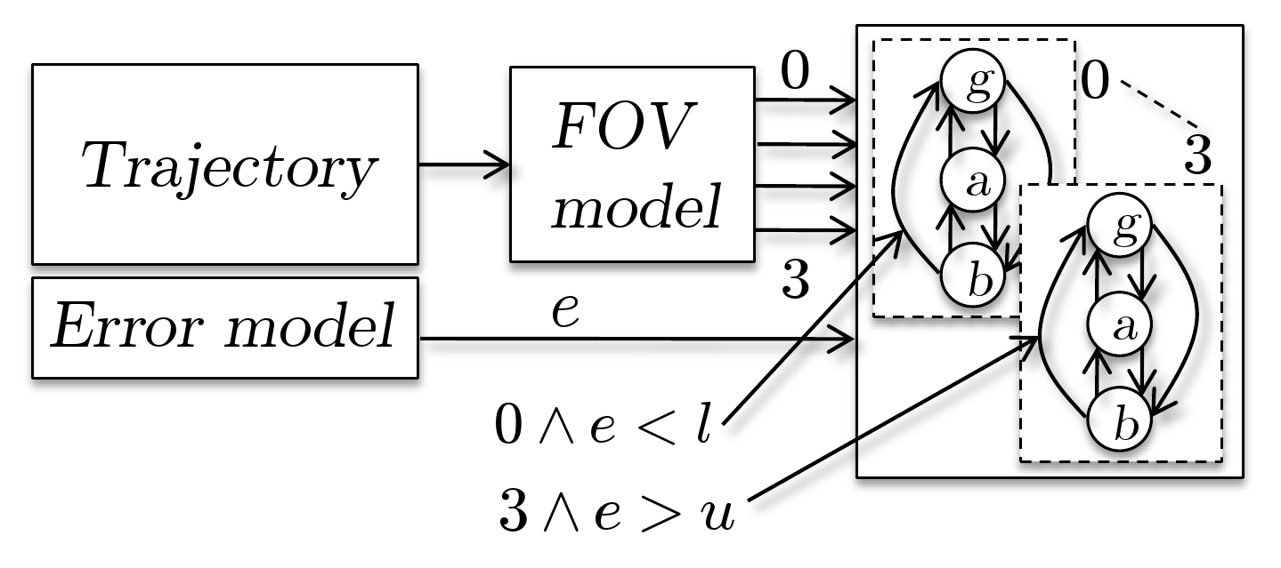
The model is shown in Figure 17²² 2 A more detailed Simulink/Stateflow model can be found in [66] and has two parts. The trajectory followed by the helicopter is computed by a trajectory generation algorithm for given way-points around the building. A camera model is used to generate Boolean flags that are equal to TRUE if the corresponding object is in the field of view of the camera and FALSE otherwise (Field of view model). The vision algorithm is a finite state model that maintains a matching score for each of the objects in the scene (the object being parallel states). When in the field of view, the score assigned to object $0$ increases if the position error is below a lower bound $l$ , and decreases if it is above an upper bound $u$ (transitions are reversed for the other objects). Because the update is done at each frame, higher computation rates improve the ability to distinguish image features. The system is translated into a SAN, where the variance $\sigma$ of the colored noise $e$ is one of the parameters. The transition rate $\lambda$ associated with transitions in the vision algorithm model is another parameter. These two parameters represent the accuracy of the sensors and the speed of execution (i.e. frames per second) of the vision algorithm, respectively. The helicopter follows a circular trajectory around the building. We report the values of the probability of being in each of the three level of the matching score for all the objects in Table 1.

$(\lambda,\sigma)$	Score	0	1	2	3
	$g$	0.6207	0.0254	0.0110	0.0241
$(0.5,0.21)$	$a$	0.1846	0.1823	0.1792	0.1805
	$b$	0.1946	0.7923	0.8098	0.7954
	$g$	0.5561	0.0472	0.0381	0.0456
$(1,0.42)$	$a$	0.3821	0.3741	0.3806	0.3738
	$b$	0.0617	0.5787	0.5813	0.5806
	$g$	0.4071	0.1424	0.1401	0.1423
$(10,0.84)$	$a$	0.4533	0.4527	0.4526	0.4529
	$b$	0.1396	0.4048	0.4073	0.4047

Table 1: Probabilities of good, average and bad matching for different values of error variance and computation speed.

Recently we have also addressed the synthesis problem of designing a control strategy for a vehicle that provides probabilistic guarantees of accomplishing the mission in a hostile environment with obstacles and moving adversaries [11]. The vehicle is required to satisfy a mission objective expressed as a temporal logic specification over a set of properties satisfied at regions of a partitioned environment. We capture the motion of the vehicle and the vehicle updates of adversaries distributions as a Markov Decision Process. In particular, we abstract the probability of a vehicle computing a feasible path and avoiding obstacles over a region under assumption that the trajectory planner is using a sampling-based motion planning algorithm such as one described in Section 4. Using tools in Probabilistic Computational Tree Logic, we find a control strategy for the vehicle that maximizes the probability of accomplishing the mission objective. For details reader is referred to [11].

Example of architectural analysis

We consider a distributed architecture composed of processors running a single thread and communicating over a token ring bus (details can be found in [56]). Each thread $th_{i}$ has three states: a $sleep$ state where the thread is not active, a $ready$ state where the thread is ready to be executed by the processor is busy, and a $run$ state where the thread is running. The thread transitions from the $sleep$ state to the $ready$ state when its transmission buffer $TX_{i}$ is empty. When the thread is scheduled to run, it first reads from buffer $RX_{i}$ , and then writes its transmission buffer $TX_{i}$ . A token ring bus serves the TX buffers and broadcasts their content to all RX buffers in the system. We consider transition rates of $10^{5}$ , $10^{4}$ and $10^{3}$ for transitions $(sleep,ready)$ , $(ready,run)$ and $(run,sleep)$ respectively. We also consider a rate of $8000$ for the protocol to pass the token among users, while we leave the data transmission rate $\lambda$ as a parameter (to mimic the effect of different packet sizes). We consider three architectures: $sys2$ with two processors ( $182$ reachable states), $sys4$ with four processors ( $24708$ reachable states) and $sys4f$ with 4 unreliable processors ( $2118680$ reachable states). Unreliable processors can fail with rate $0.0003$ , and recover from failure with rate $0.3$ . The results of the analysis are shown in Table 2 where we report the probability of being in the sleep, ready or run state for thread $th_{2}$ at time $t=1ms$ .

$\lambda$	System	$P(sleep)$	$P(ready)$	$P(run)$
	$sys2$	0.275	0.058	0.666
8000	$sys4$	0.380	0.038	0.581
	$sys4f$	0.371	0.038	0.591
	$sys2$	0.378	0.040	0.581
4000	$sys4$	0.453	0.025	0.522
	$sys4f$	0.439	0.025	0.535
	$sys2$	0.459	0.026	0.515
2000	$sys4$	0.505	0.016	0.479
	$sys4f$	0.489	0.016	0.495

Table 2: Probabilities of being in the sleep, ready or run state at

t=1ms

for thread

th_{2}

The results show two obvious trends. When the number of processors increases, the token rotation time increases and the time a task spends in the sleep state also increases. If the transmission time increases, the time spent in the sleep state also increases. Interestingly, the time spent in the run state is higher for $sys4f$ than for $sys4$ . This is because thread $th_{2}$ can leverage the time when other processors are silent because of a failure.

7 Conclusions

In this paper we have overviewed some recent advances in methodology and tools to model, analyze, and design interconnected dynamical systems with emphasis on robust autonomous aerospace systems operating in uncertain environment. The key idea that enables scalable computation and analysis is the decomposition of the large interconnected systems into weakly interacting subnetworks. We reviewed a new graph decomposition method based on wave equation based clustering to identify such weakly interacting subnetworks in a scalable manner. We showed how this decomposition can be exploited to accelerate uncertainty quantification in the probabilistic waveform relaxation approach. We also addressed another aspect of uncertainty management: design of search and tracking algorithms for unmanned aerospace systems that allow optimal uncertainty reduction in location of stationary and mobile targets in search and tracking problems. We described a novel ergodic dynamical system theory based sensor resource management approach for such applications. Robust motion planning using probabilistic roadmap was also demonstrated for realistic vehicle dynamics in an obstacle rich environment. Building on these approaches which apply to a specific abstraction level, we presented a general unified abstraction-based methodology and tools for analysis and synthesis for uncertain systems. We demonstrated the efficient uncertainty quantification and robust design using the case studies of model-based target tracking and search, and mission planning in an obstacle rich environment. To show the generality of our methodology we also considered problem of uncertainty quantification in energy usage in buildings, and stability assessment of interconnected power networks. We also briefly identified several challenges and promising future directions for each methodology and tool.

8 Acknowledgement

This work was supported in part by DARPA DSO under AFOSR contract FA9550-07-C-0024, Robust Uncertainty Management (RUM). Any opinions, findings and conclusions or recommendations expressed in this material are those of the author(s) and do not necessarily reflect the views of the AFOSR or DARPA. The authors will like to thank Jerrold E. Marsden, Matthew West, Sean P. Meyn, Calin Belta, Michael Dellnitz, Sudha Krishnamurthy, Suresh Kannan, Konda Reddy Chevva, Sanjay Bajekal, Sophie Lorie and Jose M. Pasini, for useful discussions and feedback. We would especially like to acknowledge the profound influence that Jerry Marsden had on this research direction and on many of us personally. Jerry brought to us the idea of using graph decomposition to break the complexity of computations and analysis in uncertain dynamic networks, the key idea behind the RUM project. In fact, Jerry was the person who invented the acronym DyNARUM (Dynamic Network Analysis for Robust Uncertainty Management), which was how we internally called the RUM project. Jerry Marsden was also one of the champions of using precomputed piecewise optimal motion primitives. Finally, Jerry Marsden has personally inspired many of us to pursue some the key research ideas included in this paper. We called the positive influence of the discussions with Jerry Marsden that stayed with us for a long time after the discussions and kept us pursuing the research with hope and excitement “the Jerry effect”. This paper is a result of the “Jerry effect” that is still within us.

References

[1] 3rd Workshop on High-Dimensional Approximation. http://conferences.science.unsw.edu.au/hda09/. Feb, Sydney, Australia 2009.
[2] A. Abate, J.P Katoen, J. Lygeros, and M. Prandini. Approximate model checking of stochastic hybrid systems. European Journal of Control, 2010. Provisionally Accepted.
[3] Luca De Alfaro. Model checking of probabilistic and nondeterministic systems. In Foundations of Software Technology and Theoretical Computer Science, pages 499–513. Springer-Verlag, 1995.
[4] C. Baier. On Algorithmic Verification Methods for Probabilistic Systems. PhD thesis, University of Mannheim, 1998.
[5] A. Banaszuk and J. Pasini. Robust uncertainty management, darpa dso final report. Technical report, UTRC, 2009.
[6] Gunter Bolch, Stefan Greiner, Hermann de Meer, and Kishor Shridharbhai Trivedi. Queueing Networks and Markov Chains. Wiley-Interscience, 2005.
[7] Randal E. Bryant. Graph-based algorithms for boolean function manipulation. IEEE Trans. Comput., 35(8):677–691, 1986.
[8] Francesco Bullo and Andrew Lewis. Geometric Control of Mechanical Systems. Springer, 2004.
[9] Howie Choset, Kevin M. Lynch, Seth Hutchinson, George A Kantor, Wolfram Burgard, Lydia E. Kavraki, and Sebastian Thrun. Principles of Robot Motion: Theory, Algorithms, and Implementations. MIT Press, June 2005. ISBN 0-262-03327-5.
[10] F. R. K. Chung. Spectral Graph Theory. American Mathematical Society, first edition, 1997.
[11] Igor Cizelj, Xu Chu (Dennis) Ding, Morteza Lahijanian, Alessandro Pinto, and Calin Belta. Probabilistically safe vehicle control in a hostile environment. submitted to IFAC, 2010.
[12] Francis H. Clarke, Yuri S. Ledyaev, Ronald J. Stern, and Peter R. Wolenski. Nonsmooth Analysis and Control Theory. Springer, 1998.
[13] J. Cortes, S. Martinez, T. Karatas, and F. Bullo. Coverage control for mobile sensing networks. IEEE Transactions of Robotics and Automation, 20(2):243–255, 2004.
[14] L. C. Evans. Partial Differential Equations. American Mathematical Society, 1998.
[15] M. Fiedler. Algebraic connectivity of graphs. Czechoslovak Mathematical Journal, 23:289–305, 1973.
[16] M. Fiedler. A property of eigenvectors of nonnegative symmetric matrices and its application to graph theory. Czechoslovak Mathematical Journal, 25(4):619–633, 1975.
[17] G. Fishman. Monte Carlo: Concepts, Algorithms, and Applications. Springer-Verlag, New York, 1996.
[18] J. Foo, X. Wan, and G. Karniadakis. The multi-element probablistic collocation method (me-pcm): Error analysis and applications. Journal Of Computational Physics, 227(22):9572–9595, 2008.
[19] E. Frazzoli, M. A. Dahleh, and E. Feron. Maneuver-based motion planning for nonlinear systems with symmetries. IEEE Transactions on Robotics, 21(6):1077–1091, dec 2005.
[20] J. Friedman and J. P. Tillich. Wave equations for graphs and edge-based Laplacians. Pacific Journal of Mathematics, 216(2):229–266, 2004.
[21] T. T. Georgiou and M. C. Smith. Linear systems and robustness -a graph point of view. Lecture Notes in Control and Information Sciences, 183:114–121, 1992.
[22] T. Gerstner and M. Griebel. Numerical integration using sparse grids. Numerical Algorithms, 18(3-4):200–, 1998.
[23] G. Golub and C. Van Loan. Matrix Computations. John Hopkins University Press, 1996.
[24] S. Gottschalk, M. C. Lin, and D. Manocha. OBBTree: A hierarchical structure for rapid interference detection. Eurographics/ACM SIGGRAPH Symposium on Computer Animation, 30:171–180, 1996.
[25] Andrew Howard, Maja J. Mataric, and Gaurav S Sukhatme. Mobile sensor network deployment using potential fields: A distributed, scalable solution to the area coverage problem. In Proceedings of the 6th International Symposium on Distributed Autonomous Robotics Systems, pages 299–308, 2002.
[26] J. Hu, J. Lygeros, and S. Sastry. Towars a theory of stochastic hybrid systems. Proceedings of the Third international Workshop on Hybrid Systems: Computation and Control, N. A. Lynch and B. H. Krogh, Eds. Lecture Notes In Computer Science, vol. 1790. Springer-Verlag:160–173, March 2000.
[27] Alice Hubenko, Vladimir Fonoberov, George Mathew, and Igor Mezic. Multiscale adaptive search. IEEE Trans. Syst. Man Cybern. B, 2010. Accepted for publication.
[28] I. Hussein and D. Stipanović. Effective coverage control for mobile sensor networks with guaranteed collision avoidance. IEEE Transactions on Control Systems Technology, Special Issue on Multi-Vehicle Systems Cooperative Control with Applications, 15(4):642–657, 2007.
[29] S. Joe and F. Y. Kuo. Remark on algorithm 659: Implementing sobol’s quasirandom sequence generator. ACM Trans. Math. Softw., 29:49–57, 2003.
[30] M. Kac. Can one hear the shape of a drum? The American Mathematical Monthly, 73(4):1–23, 1966.
[31] D. Kartson, G. Balbo, S. Donatelli, G. Franceschinis, and G. Conte. Modelling with Generalized Stochastic Petri Nets. John Wiley & Sons, Inc., 1994.
[32] D. Kempe and F. McSherry. A decentralized algorithm for spectral analysis. Journal of Computer and System Sciences, 74(1):70–83, 2008.
[33] Peter E. Kloeden and Eckhard Platen. Numerical Solution of Stochastic Differential Equations. Springer-Verlag, 1999.
[34] M. Kobilarov. Discrete Geometric Motion Control of Autonomous Vehicles. PhD thesis, University of Southern California, 2008.
[35] Xenofon D. Koutsoukos, Senior Member, and Derek Riley. Computational methods for verification of stochastic hybrid systems. IEEE Transactions on Systems, Man, and Cybernetics - Part A, 2008.
[36] A. Lancichinetti, S. Fortunato, and F. Radicchi. Benchmark graphs for testing community detection algorithms. Physical Review E, 78:046110, 2008.
[37] J.-C. Latombe. Robot Motion Planning. Kluwer Academic Press, 1991.
[38] S. M. LaValle. Planning Algorithms. Cambridge University Press, Cambridge, U.K., 2006.
[39] Francois Lekien and Naomi Leonard. Non-uniform coverage and cartograms. SIAM Journal on Control and Optimization, 48(1):351–372, 2009.
[40] E. Lelarasmee. The waveform relaxation method for time domain analysis of large scale integrated circuits: Theory and applications. Technical Report Memorandum No. UCB/ERL M82/40, UC Berkeley, 1982.
[41] Naomi Leonard, Derek Paley, Francois Lekien, Rodolphe Sepulchre, David Fratantoni, and Russ Davis. Collective motion, sensor networks, and ocean sampling. Proceedings of the IEEE, 95(1):48–74, 2007.
[42] U. V. Luxburg. A tutorial on spectral clustering. Technical Report Technical Report No. TR-149, Max Planck Institute for Biological Cybernetics, Aug 2006.
[43] M. M. Callier, W. S. Chan, and C. A. Desoer. Input-output stability theory of interconnected systems using decomposition techniques. IEEE Transactions on Circuits and Systems, 23(12):714–729, 1976.
[44] J.E. Marsden and M. West. Discrete mechanics and variational integrators. Acta Numerica, 10:357–514, 2001.
[45] George Mathew and Igor Mezić. Spectral multiscale coverage: A uniform coverage algorithm for mobile sensor networks. In IEEE Conf. on Decision and Control, Shanghai, China, December 2009.
[46] George Mathew and Igor Mezic. Metrics for ergodicity and design of ergodic dynamics for multi-agent systems. Physica D: Nonlinear Phenomena, 2010. Accepted for publication.
[47] George Mathew and Alessandro Pinto. Markov modeling of stochastic hybrid systems. In Allerton, September 2010.
[48] George Mathew, Amit Surana, and Igor Mezić. Uniform coverage control of mobile sensor networks for dynamic target detection. In IEEE Conf. on Decision and Control, Atlanta, Georgia, USA, December 2010.
[49] I. Mezic. Coupled nonlinear dynamical systems: Asymptotic behavior and uncertainty propagation. In 43rd IEEE Conference on Decision and Control, 2004.
[50] B. Mohar. The Laplacian spectrum of graphs. Technical report, Department of Mathematics, Simon Fraser University, Canada, 1991.
[51] B. Nadler, S. Lafon, R. R. Coifman, and I. G. Kevrekidis. Diffusion maps, spectral clustering and eigenfunctions of Fokker-Planck operators. Advances in Neural Information Processing Systems, 18, 2006.
[52] B. Nadler, S. Lafon, R. R. Coifman, and I. G. Kevrekidis. Diffusion maps, spectral clustering and reaction coordinates of dynamical systems. Applied and Computational Harmonic Analysis: Special Issue on Diffusion Maps and Wavelets, 21:113–127, 2006.
[53] H. Niederreter. Random Number Generation and Quasi-Monte Carlo Methods. SIAM, Philadelphia, PA, 1992.
[54] Zheng O’Neil, Satish Narayanan, and Rohini Brahme. Model-based thermal load estimation in buildings. In SimBuild, 4th National Conference of IBIPSA-USA, 2010.
[55] David Anthony Parker. Implementation of symbolic model checking for probabilistic systems. Technical report, University of Birmingham, 2002.
[56] Alessandro Pinto and Sudha Krishnamurthy. Developing design tools for uncertain systems in an industrial setting. In Allerton, September 2010.
[57] Alessandro Pinto, Sudha Krishnamurthy, and Suresh Kannan. A model-based end-to-end toolchain for the probabilistic analysis of complex systems. In Proceedings of the 6th IEEE Conference on Automation Science and Engineering, 2010.
[58] B. Plateau and K. Atif. Stochastic automata network of modeling parallel systems. IEEE J SE, 17(10):1093–1108, October 1991.
[59] T. Sahai, A. Speranzon, and A. Banaszuk. Wave equation based algorithm for distributed eigenvector computation. In IEEE Conference on Decision and Control and Chinese Control Conference, 2010.
[60] I. H. Sloan and S. Joe. Lattice Methods for Multiple Integration. xford University Press, Oxford, 1994.
[61] I. M. Sobol. Global sensitivity indices for nonlinear mathematical models and their monte carlo estimates. Mathematics and Computers in Simulation, 55:271–280, 2001.
[62] Fabio Somenzi. Cudd: Cu decision diagram package release 2.2.0, 1998.
[63] D. A. Spielman and S.-H. Teng. Nearly-linear time algorithms for graph partitioning, graph sparsification, and solving linear systems. In Proceedings of the thirty-sixth annual ACM symposium on Theory of computing, pages 81–90, 2004.
[64] Michael Stamatelatos and William Vesely. Fault tree handbook with aerospace applications. NASA Office of Safety and Mission Assurance, 2002.
[65] H. Stark and J.W. Wood. Probability, Random Processes, and Estimation Theory for Engineers. Prentice Hall, 2002.
[66] Suresh Kannan Sudha Krishnamurthy, Alessandro Pinto. A model-based end-to-end toolchain for the probabilistic analysis of complex systems. In Proceedings of the 6th IEEE Conference on Automation Science and Engineering (CASE), August 2010.
[67] Amit Surana and Andrzej Banaszuk. Scalable uncertanity quantification in complex dynamic networks. In IEEE Conf. on Decision and Control, Atlanta, Georgia, USA, December 2010.
[68] U. Trottenberg, C. W. Oosterlee, and A. Schüller. Multigrid. Academic Press, 2001.
[69] U. v. Luxburg, O. Bousquet, and M. Belkin. On the convergence of spectral clustering on random samples: the normalized case. In Proceedings of the 17th Annual Conference on Learning Theory (COLT), pages 457–471, 2004.
[70] S. Varigonda, T. Kalmar-Nagy, B. Labarre, and I. Mezic. Graph decomposition methods for uncertainty propagation in complex, nonlinear interconnected dynamical systems. IEEE Conference on Decision and Control, 2:1794–1798, 2004.
[71] U. von Luxburg. A tutorial on spectral clustering. Statistics and Computing, 17:395–416, 2007.
[72] J.K. White and A. S. Vincentelli. Relaxation techniques for the simulation of VLSI circuits. Kluwer International Series In Engineering And Computer Science, 1987.
[73] D. Xiu. Efficient collocational approach for parametric uncertanity analysis. Communications in Computational Physics, 2(2):293, 2007.
[74] D. Xiu and G. Karniadakis. The wiener-askey polynomial chaos for stochastic differential equations. SIAM J. Sci. Comput., 24:619–644, 2002.