Maxwell’s equations for magnets

Gauss’s theorem states that for any smooth vector field $\vec{a}$:

$$\int_{V}\nabla\cdot\vec{a}\,dV=\int_{\partial V}\vec{a}\cdot d\vec{S},$$

where $V$ is a volume bounded by the closed surface $\partial V$. Note that the area element $d\vec{S}$ is oriented to point out of $V$.

Gauss’s theorem is helpful for obtaining physical interpretations of two of Maxwell’s equations, (1) and (2). First, applying Gauss’s theorem to (1) gives:

$$\int_{V}\nabla\cdot\vec{D}\,dV=\int_{\partial V}\vec{D}\cdot d\vec{S}=q,$$

(6)

where $q=\int_{V}\rho\,dV$ is the total charge enclosed by $\partial V$.

Suppose that we have a single isolated point charge in an homogeneous, isotropic medium with constant permittivity $\varepsilon$. In this case, it is interesting to take $\partial V$ to be a sphere of radius $r$. By symmetry, the magnitude of the electric field must be the same at all points on $\partial V$, and must be normal to the surface at each point. Then, we can perform the surface integral in (6):

$$\int_{\partial V}\vec{D}\cdot d\vec{S}=4\pi r^{2}D.$$

This is illustrated in Fig. 1: the outer circle represents a cross-section of a sphere ($\partial V$) enclosing volume $V$, with the charge $q$ at its centre. The black arrows in Fig. 1 represent the electric field lines, which are everywhere perpendicular to the surface $\partial V$. Since $\vec{D}=\varepsilon\vec{E}$, we find Coulomb’s law for the magnitude of the electric field around a point charge:

$$E=\frac{q}{4\pi\varepsilon r^{2}}.$$

Applied to Maxwell’s equation (2), Gauss’ theorem leads to:

$$\int_{V}\nabla\cdot\vec{B}\,dV=\int_{\partial V}\vec{B}\cdot d\vec{S}=0.$$

In other words, the magnetic flux integrated over any closed surface must equal zero—at least, until we discover magnetic monopoles. Lines of magnetic flux occur in closed loops; whereas lines of electric field can start (and end) on electric charges.

Stokes’s theorem states that for any smooth vector field $\vec{a}$:

$$\int_{S}\nabla\times\vec{a}\cdot d\vec{S}=\int_{\partial S}\vec{a}\cdot d\vec{l},$$

(7)

where the loop $\partial S$ bounds the surface $S$. Applied to Maxwell’s equation (3), Stokes’s theorem leads to

$$\int_{\partial S}\vec{H}\cdot d\vec{l}=\int_{S}\vec{J}\cdot d\vec{S},$$

(8)

which is Ampère’s law. From Ampère’s law, we can derive an expression for the strength of the magnetic field around a long, straight wire carrying current $I$. The magnetic field must have rotational symmetry around the wire. There are two possibilities: a radial field, or a field consisting of closed concentric loops centred on the wire (or some superposition of these fields). A radial field would violate Maxwell’s equation (2). Therefore, the field must consist of closed concentric loops; and by considering a circular loop of radius $r$, we can perform the integral in Eq. (8):

$$2\pi rH=I,$$

where $I$ is the total current carried by the wire. In this case, the line integral is performed around a loop $\partial S$ centred on the wire, and in a plane perpendicular to the wire: essentially, this corresponds to one of the magnetic field lines, see Fig. 2. The total current passing through the surface $S$ bounded by the loop $\partial S$ is simply the total current $I$.

In an homogeneous, isotropic medium with constant permeability $\mu$, $\vec{B}=\mu_{0}\vec{H}$, we obtain the expression for the magnetic flux density at distance $r$ from the wire:

$$B=\frac{\mu I}{2\pi r}.$$

(9)

This result will be useful when we come to consider how to generate specified multipole fields from current distributions.

Finally, applying Stokes’s theorem to the homogeneous Maxwell’s equation (4), we find

$$\int_{\partial S}\vec{E}\cdot d\vec{l}=-\frac{\partial}{\partial t}\int_{S}\vec{B}\cdot d\vec{S}.$$

(10)

Defining the electromotive force $\mathscr{E}$ as the integral of the electric field around a closed loop, and the magnetic flux $\Phi$ as the integral of the magnetic flux density over the surface bounded by the loop, Eq. (10) gives

$$\mathscr{E}=-\frac{\partial\Phi}{\partial t},$$

(11)

which is Faraday’s law of electromagnetic induction. Faraday’s law is significant for magnets with time-dependent fields, such as pulsed magnets (used for injection and extraction), and magnets that are ‘ramped’ (for example, when changing the beam energy in a storage ring). The change in magnetic field will induce a voltage across the coil of the magnet that must be taken into account when designing the power supply. Also, the induced voltages can induce eddy currents in the core of the magnet, or in the coils themselves, leading to heating. This is an issue for superconducting magnets, which must be ramped slowly to avoid quenching [6].

Gauss’s theorem and Stokes’s theorem can be applied to Maxwell’s equations to derive constraints on the behaviour of electromagnetic fields at boundaries between different materials. Here, we shall focus on the boundary conditions on the magnetic field: these conditions will be useful when we consider multipole fields in iron-dominated magnets.

Consider first a short cylinder or ‘pill box’ that crosses the boundary between two media, with the flat ends of the cylinder parallel to the boundary, see Fig. 3 (a). Applying Gauss’s theorem to Maxwell’s equation (2) gives

$$\int_{V}\nabla\cdot\vec{B}\,dV=\int_{\partial V}\vec{B}\cdot d\vec{S}=0,$$

where the boundary $\partial V$ encloses the volume $V$ within the cylinder. If we take the limit where the length of the cylinder ($2h$) approaches zero, then the only contributions to the surface integral come from the flat ends; if these have infinitesimal area $dS$, then since the orientations of these surfaces are in opposite directions on opposite sides of the boundary, and parallel to the normal component of the magnetic field, we find

$$-B_{1\perp}\,dS+B_{2\perp}\,dS=0,$$

where $B_{1\perp}$ and $B_{2\perp}$ are the normal components of the magnetic flux density on either side of the boundary. Hence

$$B_{1\perp}=B_{2\perp}.$$

(12)

In other words, the normal component of the magnetic flux density is continuous across a boundary.

A second boundary condition, this time on the component of the magnetic field parallel to a boundary, can be obtained by applying Stokes’s theorem to Maxwell’s equation (3). In particular, we consider a surface $S$ bounded by a loop $\partial S$ that crosses the boundary of the material, see Fig. 3 (b). If we integrate both sides of Eq. (3) over that surface, and apply Stokes’s theorem (7), we find

$$\int_{S}\nabla\times\vec{H}\cdot d\vec{S}=\int_{\partial S}\vec{H}\cdot d\vec{l}=I+\frac{\partial}{\partial t}\int_{S}\vec{D}\cdot d\vec{S},$$

where $I$ is the total current flowing through the surface $S$. Now, let the surface $S$ take the form of a thin strip, with the short ends perpendicular to the boundary, and the long ends parallel to the boundary. In the limit that the length of the short ends goes to zero, the area of $S$ goes to zero: both the current flowing through the surface $S$, and the electric displacement integrated over $S$ become zero. However, there are still contributions to the integral of $\vec{H}$ around $\partial S$ from the long sides of the strip. Thus we find that

$$H_{1\parallel}=H_{2\parallel},$$

(13)

where $H_{1\parallel}$ is the component of the magnetic intensity parallel to the boundary at a point on one side of the boundary, and $H_{2\parallel}$ is the component of the magnetic intensity parallel to the boundary at a nearby point on the other side of the boundary. In other words, the tangential component of the magnetic intensity $\vec{H}$ is continuous across a boundary.

We can derive a stronger constraint on the magnetic field at a boundary in the case where the material on one side of the boundary has infinite permeability (which can provide a reasonable model for some ferromagnetic materials). Since $\vec{B}=\mu\vec{H}$, it follows from (13) that

$$\frac{B_{1\parallel}}{\mu_{1}}=\frac{B_{2\parallel}}{\mu_{2}},$$

and in the limit $\mu_{2}\to\infty$, while $\mu_{1}$ remains finite, we must have

$$B_{1\parallel}=0.$$

(14)

In other words, the magnetic flux density at the surface of a material of infinite permeability must be perpendicular to that surface. Of course, the permeability of a material characterizes its response to an applied external magnetic field: in the case where the permeability is infinite, a material placed in an external magnetic field acquires a magnetization that exactly cancels any component of the external field at the surface of the material.

Our goal is to determine a current distribution that will generate a pure multipole field of specified order. As a first step, we derive the multipole components in the field around a long straight wire carrying a uniform current. We already know from Ampère’s law (9) that the field at distance $r$ from a long straight wire carrying current $I$ in free space has magnitude given by

$$B=\frac{\mu_{0}I}{2\pi r},$$

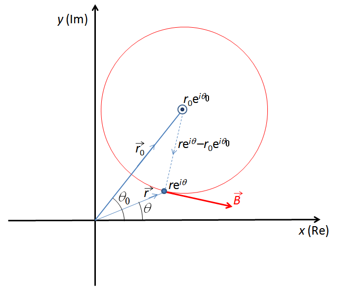
and that the direction of the field describes a circle centred on the wire. To derive the multipole components in the field, we first derive an expression for the field components at an arbitrary point $(x,y)$ from a wire carrying current $I$, passing through a point $(x_{0},y_{0})$ and parallel to the $z$ axis.

Since we are working in two dimensions, we can represent the components of a vector by the real and imaginary parts of a complex number. Thus, the vector from $(x_{0},y_{0})$ to a point $(x,y)$ is given by $re^{i\theta}-r_{0}e^{i\theta_{0}}$, and the magnitude of the field at $(x,y)$ is

$$B=\frac{\mu_{0}I}{2\pi}\,\frac{1}{\left|re^{i\theta}-r_{0}e^{i\theta_{0}}\right|}.$$

The geometry is shown in Fig. 5. The direction of the field is perpendicular to the line from $(x_{0},y_{0})$ to $(x,y)$. Since a rotation through 90^∘ can be represented by a multiplication by $i$, we can write

$$B_{x}+iB_{y}=\frac{\mu_{0}I}{2\pi}\,\frac{i\left(re^{i\theta}-r_{0}e^{i\theta_{0}}\right)}{\left|re^{i\theta}-r_{0}e^{i\theta_{0}}\right|^{2}},$$

and hence

$$B_{y}+iB_{x}=\frac{\mu_{0}I}{2\pi}\,\frac{\left(re^{-i\theta}-r_{0}e^{-i\theta_{0}}\right)}{\left|re^{i\theta}-r_{0}e^{i\theta_{0}}\right|^{2}}=\frac{\mu_{0}I}{2\pi}\,\frac{1}{re^{i\theta}-r_{0}e^{i\theta_{0}}}.$$

Now, we write the magnetic field as

$$B_{y}+iB_{x}=-\frac{\mu_{0}I}{2\pi r_{0}}\,\frac{e^{-i\theta_{0}}}{1-\frac{r}{r_{0}}e^{i(\theta-\theta_{0})}},$$

and use the Taylor series expansion for $(1-\zeta)^{-1}$, where $\zeta$ is a complex number with $|\zeta|<1$:

$$\frac{1}{1-\zeta}=\sum_{n=0}^{\infty}\zeta^{n},$$

to write

$$B_{y}+iB_{x}=-\frac{\mu_{0}I}{2\pi r_{0}}\,e^{-i\theta_{0}}\,\sum_{n=1}^{\infty}\left(\frac{r}{r_{0}}\right)^{n-1}e^{i(n-1)(\theta-\theta_{0})}.$$

(27)

Equation (27) is valid for $r<r_{0}$. Comparing with the standard multipole expansion, Eq. (26), we see that if we choose for the reference field $B_{\textrm{ref}}$ and the reference radius $R_{\textrm{ref}}$

	$\displaystyle B_{\textrm{ref}}$	$\displaystyle=$	$\displaystyle\frac{\mu_{0}I}{2\pi r_{0}},$
	$\displaystyle R_{\textrm{ref}}$	$\displaystyle=$	$\displaystyle r_{0},$

then the coefficients for the multipole components in the field are given by

$$b_{n}+ia_{n}=-e^{-in\theta_{0}}.$$

The field around a long straight wire can be represented as an infinite sum over all multipoles.

Now we consider a current flowing on the surface of a cylinder of radius $r_{0}$. Suppose that the current flowing in a section of the cylinder at angle $\theta_{0}$ and subtending angle $d\theta_{0}$ at the origin is $I\!(\theta_{0})\,d\theta_{0}$. By the principle of superposition, we can obtain the total field by summing the contributions from the currents at all values of $\theta_{0}$:

$$B_{y}+iB_{x}=-\frac{\mu_{0}}{2\pi r_{0}}\,\sum_{n=1}^{\infty}\left(\frac{r}{r_{0}}\right)^{n-1}e^{i(n-1)\theta}\int_{0}^{2\pi}e^{-in\theta_{0}}\,I\!(\theta_{0})\,d\theta_{0}.$$

(28)

We see that the multipole components are related to the Fourier components in the current distribution over the cylinder of radius $r_{0}$. In particular, if we consider a current distribution with just a single Fourier component

$$I\!(\theta_{0})=I_{0}\cos\left(n_{0}\theta_{0}-\phi\right),$$

(29)

the integral in the right-hand side of Eq. (28) vanishes except for $n=n_{0}$, and we find

$$B_{y}+iB_{x}=-\frac{\mu_{0}I_{0}}{2\pi r_{0}}\,\left(\frac{r}{r_{0}}\right)^{n_{0}-1}e^{i(n_{0}-1)\theta}\pi e^{-i\phi}.$$

The current distribution (29) generates a pure multipole field of order $n_{0}$. If we choose, as before

	$\displaystyle B_{\textrm{ref}}$	$\displaystyle=$	$\displaystyle\frac{\mu_{0}I_{0}}{2\pi r_{0}},$
	$\displaystyle R_{\textrm{ref}}$	$\displaystyle=$	$\displaystyle r_{0},$

then the multipole coefficients are

$$b_{n}+ia_{n}=-\pi e^{-i\phi}.$$

The parameter $\phi$ gives the ‘angle’ of the current distribution. For $\phi=0$ or $\phi=\pi$, the current generates a normal multipole; for $\phi=\pm\pi/2$, the current generates a skew multipole (Fig 6).

The fact that a sinusoidal current distribution on a cylinder can generate a pure multipole field is not simply of academic interest. By winding wires in an appropriate pattern on a cylinder, it is possible to approximate a sinusoidal current distribution closely enough to produce a multipole field of acceptable quality for many applications. Usually, several layers of windings are used with a different pattern of wires in each layer, to improve the approximation to a sinusoidal current distribution. Superconducting wires can be used to achieve strong fields: an example of superconducting quadrupoles in the LHC is shown in Fig. 7.

Normal-conducting magnets usually use iron cores to increase the flux density achieved by a given current. In such a magnet, the shape of the magnetic field depends mainly on the geometry of the iron. In this section, we shall derive the geometry required to generate a pure multipole of given order. To simplify the problem, we will make some approximations: in particular, we shall assume that the iron core has uniform cross-section and infinite extent along $z$; that there are no limits to the iron in $x$ or $y$; and that the iron has infinite permeability. The field in a more realistic magnet will generally need to be calculated numerically; however, the characteristics derived from our idealized model are often a good starting point for the design of an iron-dominated multipole magnet.

We base our analysis on the magnetic scalar potential, $\varphi$, which is related to the magnetic field $\vec{B}$ by

$$\vec{B}=-\nabla\varphi.$$

(30)

Note that the curl of the field in this case is zero, for any function $\varphi$: this is a consequence of the mathematical properties of the grad and curl operators. Therefore, it follows from Maxwell’s equation (3) that a magnetic field can only be derived from a scalar potential if: (i) there is no current density at the location where the field is to be calculated; (ii) there is no time-dependent electric displacement at the location where the field is to be calculated. Where there exists an electric current or a time-dependent electric field, it is more appropriate to use a vector potential (in which case, the magnetic flux density is found from the curl of the vector potential). However, for multipole fields, we have already shown that both the divergence and the curl of the field vanish, Eqs. (21) and (22). Since the curl of the grad of any function is identically zero, Eq. (22) is automatically satisfied for any field $\vec{B}$ derived using (30). From Eq. (21), we find

$$\nabla^{2}\varphi=0,$$

(31)

where $\nabla^{2}$ is the Laplacian operator. Equation (31) is Poisson’s equation: the scalar potential in a particular case is found by solving this equation with given boundary conditions.

To determine the geometry of iron required to generate a pure multipole field, we shall start by writing down the scalar potential for a pure multipole field. Since the magnetic flux density $\vec{B}$ is obtained from the gradient of the scalar potential, the flux density at any point must be perpendicular to a surface of constant scalar potential. However, we already know from Eq. (14) that the magnetic flux density at the surface of a material with infinite permeability must be perpendicular to that surface. Hence to generate a pure multipole field in a magnet containing material of infinite permeability, we just need to shape the material so that its surface follows a surface of constant magnetic scalar potential for the required field.

We therefore look for a potential $\varphi$ that satisfies

$$-\left(\frac{\partial}{\partial y}+i\frac{\partial}{\partial x}\right)\varphi=B_{y}+iB_{x}=C_{n}(x+iy)^{n-1}.$$

As we shall now show, an appropriate solution is

$$\varphi=-\left|C_{n}\right|\frac{r^{n}}{n}\sin(n\theta-\phi_{n})$$

(32)

where

$$x+iy=re^{i\theta},$$

and so

	$\displaystyle x$	$\displaystyle=$	$\displaystyle r\cos\theta,$
	$\displaystyle y$	$\displaystyle=$	$\displaystyle r\sin\theta.$

That Eq. (32) is indeed the potential for a pure multipole of order $n$ can be shown as follows. In polar coordinates, the gradient can be written

$$\nabla\varphi=\hat{r}\frac{\partial\varphi}{\partial r}+\frac{\hat{\theta}}{r}\frac{\partial\varphi}{\partial\theta},$$

(33)

where $\hat{r}$ and $\hat{\theta}$ are unit vectors in the directions of increasing $r$ and $\theta$, respectively. Using

	$\displaystyle\hat{r}$	$\displaystyle=$	$\displaystyle\hat{x}\cos\theta+\hat{y}\sin\theta,$
	$\displaystyle\hat{\theta}$	$\displaystyle=$	$\displaystyle-\hat{x}\sin\theta+\hat{y}\cos\theta,$

it follows from Eq. (33) that

	$\displaystyle-\nabla\varphi$	$\displaystyle=$	$\displaystyle(\hat{x}\cos\theta+\hat{y}\sin\theta)\left|C_{n}\right|r^{n-1}\sin(n\theta-\phi_{n})-(\hat{x}\sin\theta-\hat{y}\cos\theta)\left|C_{n}\right|r^{n-1}\cos(n\theta-\phi_{n}),$
		$\displaystyle=$	$\displaystyle\hat{x}\sin\!\left((n-1)\theta-\phi_{n}\right)\left|C_{n}\right|r^{n-1}+\hat{y}\cos\!\left((n-1)\theta-\phi_{n}\right)\left|C_{n}\right|r^{n-1}.$

Thus the field derived from the potential (32) can be written

$$B_{y}+iB_{x}=\left|C_{n}\right|e^{-i\phi_{n}}r^{n-1}e^{i(n-1)\theta}.$$

Therefore, if

$$C_{n}=\left|C_{n}\right|e^{-i\phi_{n}},$$

then

$$B_{y}+iB_{x}=C_{n}r^{n-1}e^{i(n-1)\theta}=C_{n}(x+iy)^{n-1},$$

and we see that the potential (32) does indeed generate a pure multipole field of order $n$.

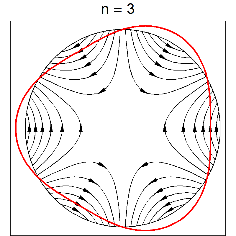
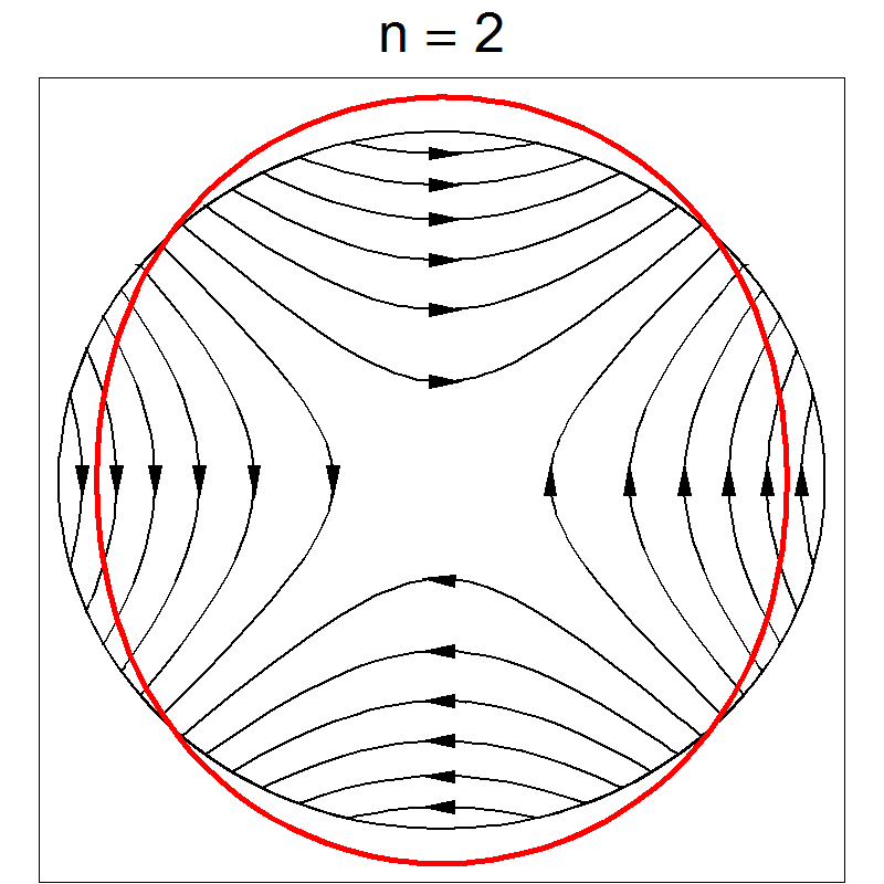
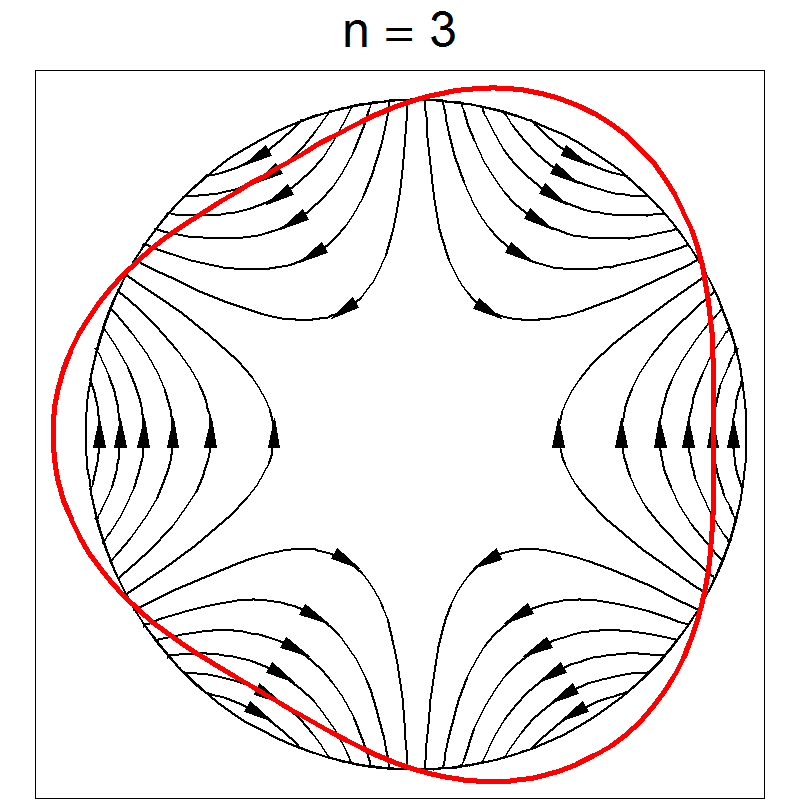
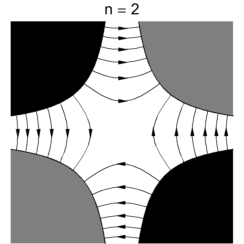
From the above argument, we can immediately conclude that to generate a pure multipole field, we can shape a high permeability material such that the surface of the material follows the curve given (in parametric form, with parameter $\theta$) by

$$r^{n}\sin(n\theta-\phi_{n})=r_{0}^{n},$$

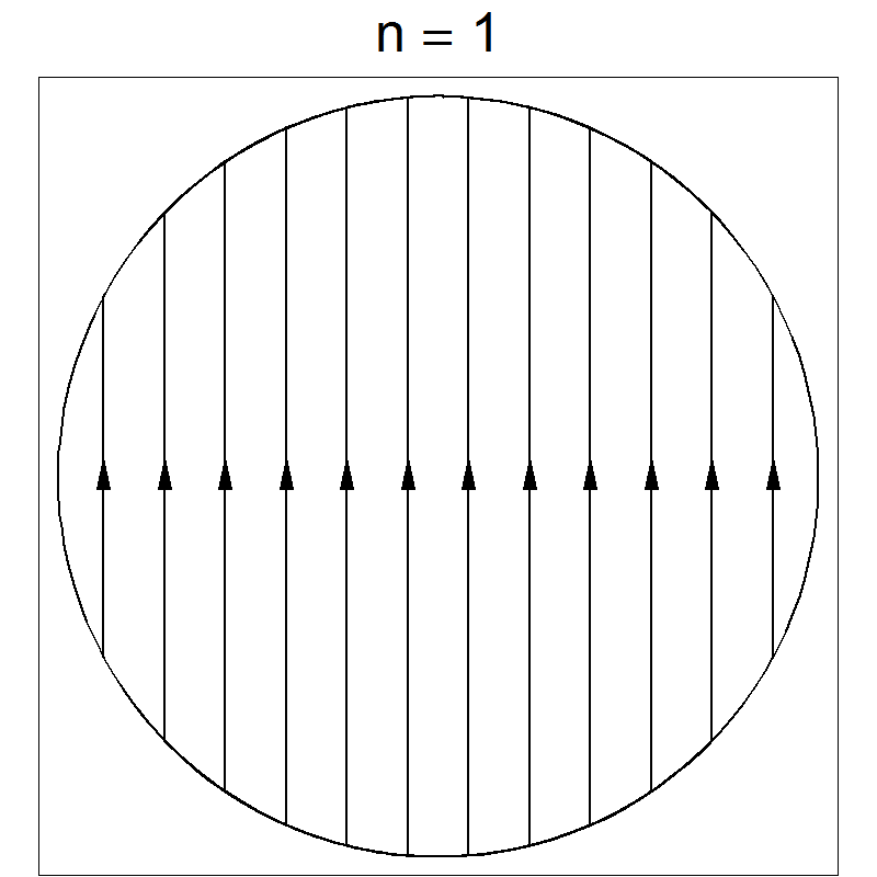
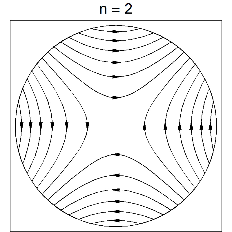
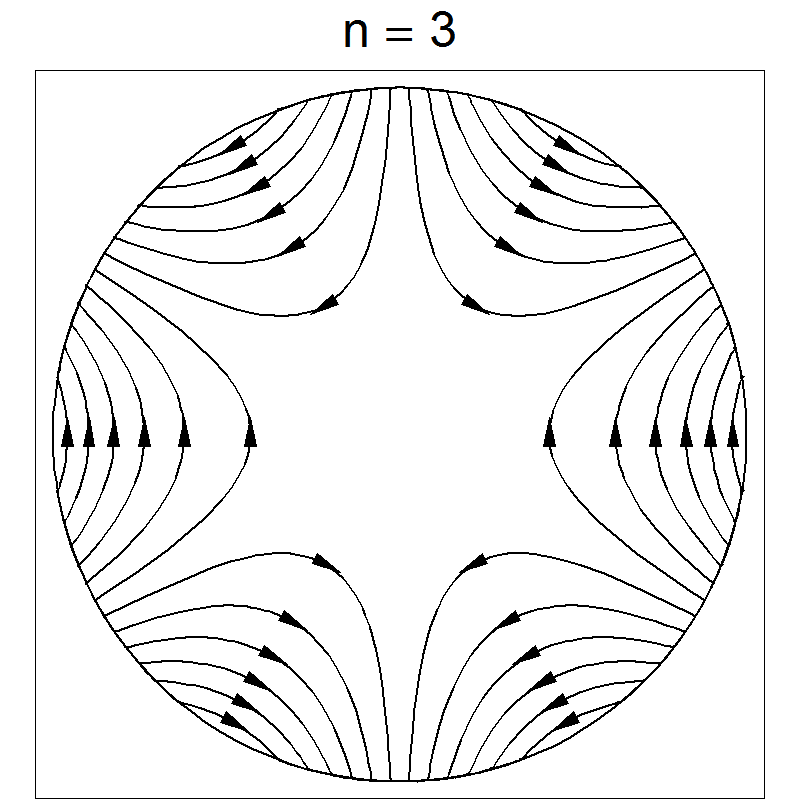
(34)

where $r_{0}$ is a constant giving the minimum distance between the surface of the material and the origin. The cross-sections of iron-dominated multipole magnets of orders 1, 2 and 3 are shown in Fig. 8. Note that $r\to\infty$ for $n\theta-\phi_{n}\to\textrm{integer}\times\pi$. Treating each region between infinite values of $r$ as a separate pole, we see that a pure multipole of order $n$ has 2$n$ poles. We also see that the potential changes sign when moving from one pole to either adjacent pole: that is, poles alternate between ‘north’ and ‘south’. The field must be generated by currents flowing along wires between the poles, parallel to the $z$ axis: to avoid direct contribution from the field around the wires, these wires should be located a large (in fact, infinite) distance from the origin.

Note that it is possible to determine the shape of the pole face for a magnet containing any specified set of multipoles by summing the potentials for the different multipole components, and then solving for $r$ as a function of $\theta$, for a fixed value of the scalar potential. Magnets designed to have more than one multipole component are often known as ‘combined function’ magnets. Perhaps the most common type of combined function magnet is a dipole with a quadrupole component: such magnets can be used to steer and focus a beam simultaneously. The shape of the pole faces and the field lines in a dipole with (strong) quadrupole component is shown in Fig. 9.

In practice, some variation from the ‘ideal’ geometry is needed to account for the fact that the material used in the magnet has finite permeability, and finite extent transversely and longitudinally. The wires carrying the current that generates the magnetic flux are arranged in coils around each pole; as we shall see, the strength of the field is determined by the number of ampere-turns in each coil. An iron-dominated electromagnetic quadrupole is shown in Fig. 10.

To complete our discussion of methods to generate multipole fields, we derive an expression for the field strength in an iron-dominated magnet with a given number of ampere-turns in the coil around each pole. To do this, we consider a line integral as shown in Fig. 11. In the figure, we show a quadrupole; however the generalization to other orders of multipole is straightforward. Note that, in principle, the coils carrying the electric current, and the line segment $C_{3}$, are an infinite distance from the origin (the centre of the magnet).

Using Maxwell’s equation (3), with constant (zero) electric displacement, and integrating over the surface $S$ bounded by the curve $C_{1}+C_{2}+C_{3}$ gives

$$\int_{S}\nabla\times\vec{H}\cdot d\vec{S}=\int_{S}\vec{J}\cdot d\vec{S}=-NI.$$

Note that the surface is oriented so that the normal is parallel to the positive $z$ axis; and the coil around each pole consists of $N$ turns of wire carrying current $I$. Applying Stokes’s theorem (7) gives

$$\int_{C_{1}}\vec{H}\cdot d\vec{l}+\int_{C_{2}}\vec{H}\cdot d\vec{l}+\int_{C_{3}}\vec{H}\cdot d\vec{l}=-NI.$$

We know, from Eq. (12), that the normal component of the magnetic flux density $\vec{B}$ is continuous across a boundary. Then, since $\vec{B}=\mu\vec{H}$, it follows that for a finite field between the poles, and for $\mu\to\infty$, the magnetic intensity $\vec{H}$ vanishes within the poles. Also, the field is perpendicular to the line segment $C_{2}$. Thus, the only part of the integral that makes a non-zero contribution, is the integral along $C_{1}$ from the face of the pole to the origin. Hence

$$\int_{0}^{r_{0}}\frac{B_{r}(r)}{\mu_{0}}dr=NI.$$

(35)

The contour $C_{1}$ is chosen so that along this contour the field has only a radial component, parallel to the contour. From Eq. (24), we see that for a multipole of order $n$, along this contour we have

$$B_{r}=\left|C_{n}\right|r^{n-1}.$$

Thus we find by performing the integral in Eq. (35)

$$\left|C_{n}\right|=\mu_{0}NI\frac{n}{r_{0}^{n}}.$$

For a normal multipole, the field is given by

$$B_{y}+iB_{x}=\frac{\mu_{0}nNI}{r_{0}}\left(\frac{x+iy}{r_{0}}\right)^{n-1}.$$

For example, in a normal quadrupole ($n=2$), the field gradient is given by

$$\frac{\partial B_{y}}{\partial x}=\frac{2\mu_{0}NI}{r_{0}^{2}}.$$

(36)

A pure multipole field of order $n$ can be written

$$B_{y}+iB_{x}=\left|C_{n}\right|e^{-i\phi_{n}}r^{n-1}e^{i(n-1)\theta}.$$

(37)

The parameter $\phi_{n}$ characterizes the angular orientation of the magnet around the $z$ axis. In particular, from Eq. (34), we see that a change in $\phi_{n}$ by $n\alpha$ is equivalent to a rotation of the coordinates (a change in $\theta$) by $-\alpha$. Thus, a rotation of a magnet around the $z$ axis by angle $\alpha$ may be represented by a change in $\phi_{n}$ by $n\alpha$. In particular, if the magnet is rotated by $\pi/n$, then from Eq. (37), we see that the field at any point simply changes sign:

$$\textrm{if }\phi_{n}\mapsto\phi_{n}+\pi,\textrm{ then }\vec{B}\mapsto-\vec{B}.$$

(38)

This property of the magnetic field is imposed by the symmetry of the magnet. In a real magnet, it will not be satisfied exactly, because random variations in the geometry will break the symmetry. However, it is possible to maintain the symmetry exactly in the design of the magnet; this means that although higher order multipoles will in general be present, only those multipoles satisfying the symmetry constraint (38) can be present. These are the ‘allowed’ multipoles. Other multipoles, which must be completely absent, are the ‘forbidden’ multipoles.

We can derive a simple expression for the allowed multipoles in a magnet designed with symmetry for a multipole of order $n$. Consider an additional multipole (a ‘systematic error’) in this field, of order $m$. By the principle of superposition, the total field can be written as

$$B_{y}+iB_{x}=\left|C_{n}\right|e^{-i\phi_{n}}r^{n-1}e^{i(n-1)\theta}+\left|C_{m}\right|e^{-i\phi_{m}}r^{m-1}e^{i(m-1)\theta}.$$

The geometry is such that under a rotation about the $z$ axis through $\pi/n$, the magnet looks the same, except that all currents have reversed direction: therefore the field simply changes sign. Under this rotation $\phi_{n}\mapsto\phi_{n}+\pi$; however, $\phi_{m}\mapsto\phi_{m}+m\pi/n$. This means that we must have:

$$e^{-i\frac{m}{n}\pi}=-1.$$

Therefore $m/n$ must be an odd integer. Assuming that $m\neq n$ (i.e., the multipole error is of a different order than the ‘main’ multipole field), then

$$\frac{m}{n}=3,5,7,\dots$$

(39)

Thus, for a dipole, the allowed higher order multipoles are sextupole, decapole, etc.; for a quadrupole, the allowed higher order multipoles are dodecapole, 20-pole, etc. The fact that the allowed higher order multipoles have an order given by an odd integer multiplied by the order of the main multipole is a consequence of the fact that magnetic poles always occur in north–south pairs. This is illustrated for a quadrupole in Fig. 12; here we see that to maintain the correct rotational symmetry (with the field changing sign under a rotation through $\pi/2$) the first higher-order multipole must be constructed by ‘splitting’ each main pole into three, then into five, and so on.

The field in a real magnet will contain all higher order multipoles, not just the ones allowed by symmetry. However, it is often the case that the allowed multipoles dominate over the forbidden multipoles.

Suppose we have obtained a set of numerical field data, either from a magnetic model, or from measurements on a real magnet. To determine the effect of the field on the beam dynamics in an accelerator, it is helpful to know the multipole components in the field. One way to compute the multipole components is to fit a polynomial to the field data. For example, if we consider a normal multipole (coefficients $C_{n}$ are all real), the vertical field along the $x$ axis (i.e., for $y=0$) is given by

$$B_{y}=\sum_{n=1}^{\infty}C_{n}x^{n-1}.$$

(40)

The number of data points determines the highest order multipole that can be fitted. Fitting may be achieved using, for example, a routine that minimizes the squares of the residuals between the data and the fitted function. However, although this procedure can, in principle, produce good results, it is not very robust. In particular, the presence of multipoles of higher order than those included in the fit can affect the values determined for those multipoles that are included in the fit. We can illustrate this as follows.

Let us construct a quadrupole field ($n=$2), and add to it higher order multipoles of order 3, 4, 5 and 6. The values of the coefficients $a_{n}$ (actual values, and fitted values in two different cases) are given in Table 1. The field $B_{y}/B_{\textrm{ref}}$ is plotted as a function of $x/R_{\textrm{ref}}$ in Fig. 13: the field data are shown as points, while the fit, including multipoles up to order 6, is shown as a line. Also shown is the deviation $\Delta B_{y}/B_{\textrm{ref}}$ from an ideal quadrupole field, i.e. $\Delta B_{y}$ is the contribution of the higher order multipoles. We see that if we base the fit on all the multipoles that are present (i.e. up to order 6), then we obtain accurate values for all multipole coefficients.

However, in general, multipoles of all orders are present, while our fit is based on a finite number of multipoles. If we try to fit the data in our illustrative case using multipoles up to order 5 only (i.e. omitting the order 6 multipole that is present), then we see that there is an impact on the accuracy with which we determine the lower-order multipoles. This can be seen in the final column of Table 1: there is even an error in the value that we determine for the quadrupole strength. When we plot the fit against the field data, we see that there is some small residual deviation between the data and the fit: this is to be expected, since the function we are using to obtain the fit does not match exactly the function used to generate the data. Although not visible in the total field, plotted in Fig. 14, the difference between the fit and the data is apparent in the plot of the deviation from the quadrupole field.

Our concern is that the presence of higher-order multipoles has affected the accuracy with which we determine the lower-order multipoles, even down to the quadrupole field strength. This can have significant implications for beam dynamics: the effect of a linear focusing error in a beam line (from some variation in the quadrupole strength) can be very different from the effects of higher-order multipole errors. For example, if one is measuring the betatron tunes or the beta functions in a storage ring, these can be very sensitive to linear focusing errors, and relatively insensitive to higher order multipoles. Determining the multipole coefficients using a polynomial fit can lead to inaccurate predictions of the linear behaviour of the beam line, depending on the higher-order multipoles present in the magnets.

The problem is that we have based our fit on monomials, i.e., powers of $x$. Our fit is a sum of these monomials, with coefficients determined from the data. However, it is possible to obtain a fit to data generated using one monomial, with a different monomial. For example, if one constructs data which is purely linear in $x$, then one can obtain a fit using a monomial $x^{3}$ (even though the fit will not be as good as one obtained using a monomial $x$). Mathematically, the basis functions we are using (monomials in this case) are not orthogonal: the coefficients we determine depend on which set of basis functions we choose to use. A more robust technique would use basis functions that are orthogonal, i.e., the coefficients we determine will be the same, no matter which set of functions we choose. Fortunately, there exists an appropriate set of functions that provides an orthogonal basis for multipole fields. We discuss this basis in the following section, 0.5.3. The advantage of orthogonal basis functions is that the coefficients we determine for different terms in the fit are independent of which terms we include in the fit; for example, the quadrupole strength that we find in a particular magnet will be the same, irrespective of which higher-order terms we include in the fit, and which higher-order terms are actually present.

From Eq. (24) we know that the field in a multipole magnet can be written in polar coordinates as

$$B_{\theta}+iB_{r}=\sum_{n=1}^{\infty}C_{n}r^{n-1}e^{in\theta}.$$

We see that if we make a set of measurements of $B_{r}$ and $B_{\theta}$ at different values of $\theta$ and fixed radial distance $r$, then we can obtain the coefficients $C_{n}$ by a discrete Fourier transform.

Suppose we make $M$ measurements of the field, at $\theta=\theta_{m}$, where

$$\theta_{m}=2\pi\frac{m}{M},\qquad m=0,1,2\dots M-1.$$

(41)

We write the measurement at $\theta=\theta_{m}$ as $B_{m}$; note that $B_{m}$ is a complex number, whose real and imaginary parts are given by the azimuthal and radial components of the field at $\theta=\theta_{m}$.

Now we construct, for a chosen integer $n^{\prime}$

$$\sum_{m=0}^{M-1}B_{m}e^{-2\pi in^{\prime}\frac{m}{M}}=\sum_{m=0}^{M-1}\sum_{n=1}^{\infty}C_{n}r_{0}^{n-1}e^{2\pi i(n-n^{\prime})\frac{m}{M}},$$

where $r_{0}$ is the radial distance at which the field measurements are made. The summation over $m$ on the right-hand side vanishes, unless $n=n^{\prime}$. Thus we can write

$$\sum_{m=0}^{M-1}B_{m}e^{-2\pi in^{\prime}\frac{m}{M}}=MC_{n^{\prime}}r_{0}^{n^{\prime}-1}.$$

If we relabel $n^{\prime}$ as $n$, then we see that the multipole coefficients $C_{n}$ are given by

$$C_{n}=\frac{1}{Mr_{0}^{n-1}}\sum_{m=0}^{M-1}B_{m}e^{-2\pi in\frac{m}{M}}.$$

(42)

The advantage of this technique over that in Section 0.5.2 is that the basis functions used to construct the fit are of the form $e^{in\theta}$, for integer $n$. These functions are orthogonal: mathematically, this means that

$$\int_{0}^{2\pi}e^{in\theta}e^{-in^{\prime}\theta}\,d\theta=2\pi\delta_{nn^{\prime}},$$

where the Kronecker delta function $\delta_{nn^{\prime}}=1$ if $n=n^{\prime}$, and $\delta_{nn^{\prime}}=0$ if $n\neq n^{\prime}$. The important consequence for us is that the value we determine for any given multipole using Eq. (42) is independent of the presence of any other multipoles, of higher or lower order.

A further advantage of using the polar basis instead of the Cartesian basis comes from the dependence of the field on the radial distance. Suppose that the field data are measured (or obtained from a model) with accuracy $\Delta B_{m}$. Then the accuracy in the multipole coefficients will be

$$\Delta C_{n}\approx\frac{\Delta B_{m}}{r_{0}^{n-1}}.$$

We obtain better accuracy in the multipole coefficients if we choose the radius $r_{0}$, on which the measurements are made, to be as large as possible. Furthermore, the accuracy in the fitted field will be

$$\Delta B\approx\Delta C_{n}\left(\frac{r}{r_{0}}\right)^{n-1}.$$

We obtain improved accuracy in the field for $r<r_{0}$; but the accuracy reduces quickly (particularly for higher-order multipoles) for $r>r_{0}$. It is important to choose the radial distance $r_{0}$ large enough to enclose all particles likely to pass through the magnet, otherwise results from tracking may not be accurate.

In this section, we have considered two techniques for deriving the multipole components of two-dimensional magnetostatic fields. We have seen that while the multipole components can be obtained, in principle, from a simple least-squares fit of a polynomial to the field components along one or other of the coordinate axes, there are advantages to basing the fit on field data obtained on a circle enclosing the origin, with as large a radius as possible. In the next section, we shall see how the idea of a multipole expansion can be generalized to three dimensions, and how a multipole decomposition can be performed in that case. However, it is worth pausing to consider in a little more detail some of the reasons for wishing to represent a field as a set of (multipole) modes.

It is of course possible to represent a magnetic field using a set of numerical field data, giving the three field components on points forming a ‘mesh’ covering the region of interest. In some ways, this is a very convenient representation, since it is the one usually provided directly by a magnetic modelling code: further processing is usually required to arrive at other representations. However, while a numerical field map in two dimensions is often a practical representation, in three dimensions the amount of data in even a relatively simple magnet can become extremely large, especially if a high resolution is required for the mesh. A multipole representation, on the other hand, provides the description of a magnetic field as a relatively small set of coefficients, from which the field components at any point can be reconstructed, using the basis functions. In other words, a multipole representation is more ‘portable’ than a numerical field map.

Secondly, a representation based on a multipole expansion lends itself to further manipulation in ways that a numerical field map does not. For example, any noise in the data (from measurement or computational errors) can be ‘smoothed’ by suppression of higher-order modes. Conversely, random errors can be introduced into data based on a model with perfect symmetry by introducing multipole coefficients corresponding to ‘forbidden’ harmonics. There will of course be issues surrounding the suppression or enhancement of errors by adjusting the multipole coefficients; however, one benefit of this approach is that for any set of multipole coefficients, the field is at least a physical field, in the sense of satisfying Maxwell’s equations. The same will not usually be true if, for example, a general smoothing algorithm is applied to a numerical field map.

Finally, one of the main motivations for performing a multipole decomposition of a field is to provide data in a format appropriate for many beam dynamics codes. Accuracy is one criterion often important for beam dynamics codes: efficiency is another. Characterization of a storage ring frequently requires tracking of thousands of particles over hundreds or thousands of turns, through a beam line that can easily consist of hundreds of magnetic elements. Numerical integration of the equations of motion for a particle in a numerical field map is generally too slow to be a practical method. There are many techniques that can be used to improve the efficiency of particle tracking in accelerators: one of the most common is the ‘thin lens’ method. The dynamical effects of dipoles and quadrupoles usually need to be represented with high accuracy. Fortunately, for these magnets, it is possible to write down accurate solutions to the equations of motion in closed form, allowing tracking through a magnet of given length to be performed in a single step. The same is not true for sextupoles, or higher-order multipoles; however, it is usually sufficiently accurate to represent such magnets by a model in which the length of the magnet approaches zero, but where the integrated strength (the multipole coefficient multiplied by the length) remains constant. For such a ‘thin lens’ it is possible to write down exact solutions to the equations of motion, allowing tracking again to be performed in a single step. A quadrupole with higher-order multipole errors can be represented as a ‘long’ perfect quadrupole field, with a set of ‘thin’ multipoles at one end, or at the centre. However, construction of such a model for a tracking code requires a multipole decomposition of the field obtained from a magnet modelling code.

We should emphasize that in our discussion of multipole decomposition, here and in Sections 0.5.2 and 0.5.3, we have made no clear distinction between field data obtained from a computational model, or from measurement of a real magnet. Of course, it is much easier to obtain the data required from a computational model: it is then quite straightforward to perform the required decomposition to determine the values of the various multipole coefficients. Unfortunately, the data do not include manufacturing errors, which can be very important. Measurements provide more realistic data: however, many other issues need to be addressed, including accuracy of field measurements, alignment of the measurement instruments with respect to the magnet, etc. Such issues are beyond the scope of our discussion.

Consider the field given by

	$\displaystyle B_{x}$	$\displaystyle=$	$\displaystyle-B_{0}\frac{k_{x}}{k_{y}}\sin(k_{x}x)\sinh(k_{y}y)\sin(k_{z}z),$		(43)
	$\displaystyle B_{y}$	$\displaystyle=$	$\displaystyle B_{0}\cos(k_{x}x)\cosh(k_{y}y)\sin(k_{z}z),$		(44)
	$\displaystyle B_{z}$	$\displaystyle=$	$\displaystyle B_{0}\frac{k_{z}}{k_{y}}\cos(k_{x}x)\sinh(k_{y}y)\cos(k_{z}z).$		(45)

As may easily be verified, this field satisfies

$$\nabla\times\vec{B}=0.$$

Furthermore, the equation

$$\nabla\cdot\vec{B}=0$$

is satisfied if

$$k_{y}^{2}=k_{x}^{2}+k_{z}^{2}.$$

(46)

We conclude that, as long as the constraint (46) is satisfied, the fields (43)–(45) provide solutions to Maxwell’s equations in regions with constant permeability, and static (or zero) electric fields. Of course, it is possible to find similar sets of equations but with different ‘phase’ along each of the coordinate axes, and with the hyperbolic trigonometric function appearing for the dependence on $x$ or $z$, rather than $y$. By superposing fields, with appropriate variations on the form given by Eqs. (43)–(45), it is possible to construct quite general three-dimensional magnetic fields. For example, a slightly more general field than that given by Eqs. (43)–(45) can be obtained simply by superposing fields with different mode numbers and amplitudes:

	$\displaystyle B_{x}$	$\displaystyle=$	$\displaystyle-\int\!\!\!\int\tilde{B}(k_{x},k_{z})\frac{k_{x}}{k_{y}}\sin(k_{x}x)\sinh(k_{y}y)\sin(k_{z}z)\,dk_{x}\,dk_{z},$		(47)
	$\displaystyle B_{y}$	$\displaystyle=$	$\displaystyle\int\!\!\!\int\tilde{B}(k_{x},k_{z})\cos(k_{x}x)\cosh(k_{y}y)\sin(k_{z}z)\,dk_{x}\,dk_{z},$		(48)
	$\displaystyle B_{z}$	$\displaystyle=$	$\displaystyle\int\!\!\!\int\tilde{B}(k_{x},k_{z})\frac{k_{z}}{k_{y}}\cos(k_{x}x)\sinh(k_{y}y)\cos(k_{z}z)\,dk_{x}\,dk_{z}.$		(49)

In this form, we see already how to perform a mode decomposition, i.e., how we can determine the coefficients $\tilde{B}(k_{x},k_{z})$ as functions of the ‘mode numbers’ $k_{x}$ and $k_{z}$. If we consider in particular the vertical field component on the plane $y=y_{0}$, then we have from (48)

$$\frac{B_{y}}{\cosh(k_{y}y_{0})}=\int\!\!\!\int\tilde{B}(k_{x},k_{z})\cos(k_{x}x)\sin(k_{z}z)\,dk_{x}\,dk_{z}.$$

Hence $\tilde{B}(k_{x},k_{z})$ may be obtained from an inverse Fourier transform of $B_{y}(x,z)/\!\cosh(k_{y}y_{0})$. Given field data on a grid over $x$ and $z$, we can then perform numerically an inverse discrete Fourier transform, to obtain a set of coefficients $\tilde{B}(k_{x},k_{z})$. Note that once we have obtained these coefficients, we can then reconstruct all field components at all points in space. This is an important consequence of the strong constraints on the fields provided by Maxwell’s equations: in general, for a static field, if we know how one field component varies over a two-dimensional plane, then we can deduce how all the field components vary over all space (on and off the plane).