∎

Error analysis of a class of derivative estimators for noisy signals

Da-yan Liu Olivier Gibaru Wilfrid Perruquetti Affiliation: D.Y. Liu Affiliation: O. Gibaru Affiliation: Laboratoire de Paul Painlevé, Université de Lille 1, 59650, Villeneuve d’Ascq, France E-mail: dayan.liu@inria.fr Affiliation: Arts et Métiers ParisTech centre de Lille, Laboratory of Applied Mathematics and Metrology (L2MA), 8 Boulevard Louis XIV, 59046 Lille Cedex, France E-mail: olivier.gibaru@ensam.eu Affiliation: École Centrale de Lille, Laboratoire de LAGIS, BP 48, Cité Scientifique, 59650 Villeneuve d’Ascq, France E-mail: wilfrid.perruquetti@inria.fr Affiliation: Équipe Projet Non-A, INRIA Lille-Nord Europe Parc Scientifique de la Haute Borne 40, avenue Halley Bât.A, Park Plaza, 59650 Villeneuve d’Ascq, France.

Received: date / Accepted: date

Abstract

Recent algebraic parametric estimation techniques (see [10, 11]) led to point-wise derivative estimates by using only the iterated integral of a noisy observation signal (see [24, 25]). In this paper, we extend such differentiation methods by providing a larger choice of parameters in these integrals: they can be reals. For this, the extension is done via a truncated Jacobi orthogonal series expansion. Then, the noise error contribution of these derivative estimations is investigated: after proving the existence of such integral with a stochastic process noise, their statistical properties (mean value, variance and covariance) are analyzed. In particular, the following important results are obtained:

$a)$: the bias error term, due to the truncation, can be reduced by tuning the parameters,
$b)$: such estimators can cope with a large class of noises for which the mean and covariance are polynomials in time (with degree smaller than the order of derivative to be estimated),
$c)$: the variance of the noise error is shown to be smaller in the case of negative real parameters than it was in [24, 25] for integer values.

Consequently, these derivative estimations can be improved by tuning the parameters according to the here obtained knowledge of the parameters’ influence on the error bounds.

Keywords:

Numerical differentiation Jacobi orthogonal polynomials Stochastic process Stochastic integrals Error bound

MSC

65D25 33C45 60H05 60J65

1 Introduction

Numerical differentiation is concerned with the estimation of derivatives of noisy time signals. This problem has attracted a lot of attention from different points of view: observer design in the control literature (see [4, 5, 14, 15, 17, 35]), digital filter in signal processing (see [2, 3, 6, 30, 33]) and so on. The problem of numerical differentiation is ill-posed in the sense that a small error in measurement data can induce a large error in the approximate derivatives. Therefore, various numerical methods have been developed to obtain stable algorithms more or less sensitive to additive noise. They mainly fall into five classes: the finite difference methods [16, 29, 31], the mollification methods [12, 26, 27], the regularization methods [28, 39, 37], the algebraic methods [25, 24] that are the roots of the here reported results, the differentiation by integration methods [18, 32, 38, 21], i.e. using the Lanczos generalized derivatives.

The Lanczos generalized derivative $D_{T}x$ , defined in [18] by

\forall t_{0}\in I,\ D_{T}x(t_{0})=\frac{3}{2T}\int_{-1}^{1}\tau\,x(t_{0}+T\tau)\,d\tau,

(1)

is an approximation to the first derivative of $x$ in the sense that $D_{T}x(t_{0})=x^{\prime}\left(t_{0}\right)+O(T^{2})$ , where $I$ is an open interval of $\mathbb{R}$ and $2T>0$ is the length of the integral window on which the estimates are calculated. It is aptly called a method of differentiation by integration. Rangarajana and al. [32] generalized it for higher order derivatives with

\forall t_{0}\in I,\ D_{T}^{(n)}x(t_{0})=\frac{1}{T^{n}}\int_{-1}^{1}\gamma_{n}L_{n}(\tau)\,x(t_{0}+T\tau)\,d\tau,\ n\in\mathbb{N},

(2)

where $x$ is assumed to belong to $C^{n+2}(I)$ and $L_{n}$ is the $n^{th}$ order Legendre polynomial defined on $[-1,1]$ . The coefficient $\gamma_{n}$ is equal to $\frac{1\times 3\times 5\times\cdots\times(2n+1)}{2}$ . By applying the scalar product of the Taylor expansion of $x$ at $t_{0}$ with $L_{n}$ they showed that $D_{T}^{(n)}x(t_{0})=x^{(n)}(t_{0})+O(T^{2})$ . By using Richardson extrapolation Wang and al. [38] have improved the convergence rate for obtaining high order Lanczos derivatives with the following affine schemes for any $n\in\mathbb{N}$

\forall t_{0}\in I,\ D_{T,\lambda_{n}}^{(n)}x(t_{0})=\frac{1}{T^{n}}\int_{-1}^{1}L_{n}(\tau)\left(a_{n}\,x(t_{0}+T\tau)+b_{n}\,x(t_{0}+\lambda_{n}T\tau)\right)d\tau,

(3)

where $x$ is assumed to belong to $C^{n+4}(I)$ , $a_{n}$ , $b_{n}$ and $\lambda_{n}$ are chosen such that $D_{T,\lambda_{n}}^{(n)}x(t_{0})=x^{(n)}(t_{0})+O(T^{4})$ . Recently, Liu et al. [21] further reduced the convergence rate in these high order cases by using Jacobi polynomials in their derivative estimators. Let us mention that all these previous estimators are given in the central case, $i.e.$ they use the interval $[t_{0}-T,t_{0}+T]$ to estimate the derivative value $x^{(n)}(t_{0})$ . Hence, these central estimators are only suited for off-line applications whereas causal estimators using the interval $[t_{0}-T,t_{0}]$ are well suited for on-line estimation which is of importance in signal processing, automatic control and in general in many real time applications.

Very recently, Mboup, Fliess and Join introduced in [9] and analyzed in [25, 24] a new causal and anti-causal version of numerical differentiation by integration method based on Jacobi polynomials

\forall t_{0}\in I,\hat{D}^{\mu,\kappa}_{\beta T}x^{(n)}(t_{0})=\frac{\gamma^{\mu,\kappa}_{n}}{(\beta T)^{n}}\int_{0}^{1}w^{\mu,\kappa}(\tau)P_{n}^{\mu,\kappa}(\tau)\,y(t_{0}+\beta T\tau)\,d\tau,

(4)

where $n\in\mathbb{N}$ , $y=x+\varpi$ is a noisy observation of $x$ which is assumed to be analytic, $\varpi$ denotes a noise, $T>0$ is the length of the time window for integration, $\beta=-1$ (causal version) or $\beta=1$ (anti-causal version) and $P_{n}^{\mu,k}$ is the $n^{th}$ order Jacobi polynomial defined on $[0,1]$ (see [1], [36]) by

\forall t\in[0,1],\ P_{n}^{\mu,\kappa}(t)=\sum_{s=0}^{n}\binom{n+\mu}{s}\binom{n+\kappa}{n-s}\left(t-1\right)^{n-s}\,t^{s},

(5)

associated to the weight function

w^{\mu,\kappa}(t)=t^{\kappa}(1-t)^{\mu}.

(6)

Let us mention that originally, these estimators were obtained using an algebraic setting: for this the authors applied a differential operator on a truncation of the Taylor series expansion of $x$ in the operational domain. This operator is given by

\begin{split}\Pi^{\mu,\kappa}_{n}=\frac{1}{s^{n+1+\mu}}\cdot\frac{d^{n+\kappa}}{ds^{n+\kappa}}\cdot s^{n},\ \text{ with }\kappa,\mu\in\mathbb{N},\end{split}

(7)

$s$ being the Laplace variable. It is in fact an annihilator which “kills” the undesired terms except the one we want to estimate (see [25, 24] for more details). This is the reason why, originally in [25, 24], the parameters $\kappa,\mu$ were assumed to be integers ( $\kappa,\mu,\in\mathbb{N}$ ). In that case, the coefficients

\gamma^{\mu,\kappa}_{n}=\frac{n!(\mu+\kappa+2n+1)!}{(\mu+n)!(\kappa+n)!}.

(8)

Let us emphasize that those methods, which are algebraic and non-asymptotic, exhibit good robustness properties with respect to corrupting noises, without the need of knowing their statistical properties (see [7, 8] for more theoretical details). The robustness properties have already been confirmed by numerous computer simulations and several laboratory experiments.

The derivative estimators given by (4) contain two sources of errors: the bias term error which comes from the truncation of the Taylor series expansion and the noise error contribution. Let us note that a precise analysis for the noise error contribution of a known noise has been done:

•

in [20], for a specific identification method,
•

in [19], for discrete cases by using different integration methods,
•

in [25], which shows that an affine estimator induces a small time delay in the estimates while reducing the bias term error for integer parameters $\kappa,\mu$ .

Thus, the aim of this paper is to reduce the errors of such derivative estimators.

For this, Section 2 allows $\kappa,\mu$ to be real: since the use of (7) induces some natural limitations ( $\kappa,\mu,\in\mathbb{N}$ ) we use truncated Jacobi orthogonal series to obtain a natural extension of (4). Let us recall that, in [25], such truncated Jacobi orthogonal series were shown to be related to (7) and the obtained estimators (4). Such obtained estimators are thus called minimal Jacobi estimators and are clearly rooted from [25].

After providing such extension ( $-1<\kappa,\mu\in\mathbb{R}$ ), Section 3 analyzes the bias term error: it is shown, for minimal Jacobi estimator, that if the $(n+1)^{th}$ derivative of the signal $x$ is slowly changing within the time window of observation then one can reduce the bias term error making $T\frac{\kappa+n+1}{\mu+\kappa+2n+2}$ small by tuning the parameters $T,\kappa,\mu$ . Lastly, it is shown that for affine estimator (real affine combination of the introduced minimal Jacobi estimators), the time delay can be reduced with the extended parameters comparing to the one obtained in [25].

Section 4 analyzes the noise error contribution in order to provide some guides for tuning the parameters $T,\kappa,\mu$ . For this we consider two cases: continuous and discrete cases so as to give noise error bounds by using the Bienaymé-Chebyshev inequality. In the first case for noises which are continuous parameter stochastic process with finite second moments, the mean value function and the covariance kernel of these noise error contributions are calculated leading to:

•

for noises whose mean value function and covariance kernel are polynomials of degree $r<n$ then the noise error contribution $e^{\beta T}_{\varpi}(t_{0})=0\text{ almost surely}$ ,
•

for Wiener or Poisson process some bounds are obtained for the noise error contribution: explicit for $n=1,2$ and it is shown how to deal with the general case.

The discrete case leads to similar results under some modified assumptions.

In Section 5, a parameter is introduced in order to reduce the error due to a numerical integration method when the extended parameters become negative. Then the comparisons of the Jacobi estimators with extended parameters and the ones with original parameters are finally done for the cases where the noises are respectively a white Gaussian noise and a Wiener process noise. The integral of the total square error and the classical $SNR$ are considered for these comparisons. Some interesting “delay-free” estimations in simulation results are shown.

2 Jacobi estimators

Let us start with $y=x+\varpi$ a noisy observation on a finite time open interval $I\subset\mathbb{R}^{+}$ of a real valued smooth signal $x$ which $n^{th}$ derivative has to be estimated ( $n\in\mathbb{N}$ ), and $\varpi$ denotes a noise. Let us assume that $x\in C^{n+1}(I)$ . For any $t_{0}\in I$ , we denote ${\cal D}_{t_{0}}=\{t\in\mathbb{R}^{+};t_{0}+\beta t\in I\}$ where $\beta=\pm 1$ .

In the two following subsections, we aim at extending the parameters $\kappa,\mu$ used in the estimators described by (4) from $\mathbb{N}$ to $]-1,+\infty[$ . To do so, we follow [25] by taking the truncated Jacobi orthogonal series. Let us stress that (4) leads to two families of anti-causal ( $\beta=1$ ) and causal ( $\beta=-1$ ) estimators.

Let us mention that, $\kappa\in\mathbb{R}$ means a non integer differentiation with respect to $s$ in (7) but has nothing to do with the estimation of non integer derivatives of noisy time signals. However, such estimation of non integer derivatives could be tackled by similar technics.

2.1 Minimal estimators

Since $x\in C^{n+1}(I)$ , we can take the Jacobi orthogonal series expansion of $x^{(n)}$

\begin{split}\forall t_{0}\in I,\ x^{(n)}(t_{0}+\beta Tt)=\sum_{i\geq 0}\frac{\langle P_{i}^{\mu+n,\kappa+n}(\tau),x^{(n)}(\beta T\tau+t_{0})\rangle}{\|P_{i}^{\mu+n,\kappa+n}\|^{2}}P_{i}^{\mu+n,\kappa+n}(t),\end{split}

(9)

where $t\in[0,1]$ , $\beta=\pm 1$ , $T\in{\cal D}_{t_{0}}$ , $n\in\mathbb{N}$ , and $\kappa,\mu\in]-1,+\infty[$ .

By taking the first term in (9) with $t=0$ , we get the following estimations

\begin{split}\forall t_{0}\in I,\ D^{\mu,\kappa}_{\beta T}x^{(n)}(t_{0})&=\frac{\langle P_{0}^{\mu+n,\kappa+n}(\tau),x^{(n)}(\beta T\tau+t_{0})\rangle}{\|P_{0}^{\mu+n,\kappa+n}\|^{2}}P_{0}^{\mu+n,\kappa+n}(0)\\ &=\frac{1}{B(\kappa+n+1,\mu+n+1)}\int_{0}^{1}w^{\mu+n,\kappa+n}(\tau)\,x^{(n)}(t_{0}+\beta T\tau)\,d\tau,\end{split}

(10)

where $B(\cdot,\cdot)$ is the classical Beta function. Recall the Rodrigues formula

\begin{split}\frac{d^{n}}{d\tau^{n}}\left\{(1-\tau)^{\mu+n}\tau^{\kappa+n}\right\}=(-1)^{n}n!(1-\tau)^{\mu}\tau^{\kappa}P_{n}^{\mu,\kappa}(\tau).\end{split}

(11)

Then, by taking $n$ times integration by parts and using the Rodrigues formula in (10) we get

\begin{split}\forall t_{0}\in I,\ D^{\mu,\kappa}_{\beta T}x^{(n)}(t_{0})=\frac{\gamma^{\mu,\kappa}_{n}}{(\beta T)^{n}}\int_{0}^{1}w^{\mu,\kappa}(\tau)P_{n}^{\mu,\kappa}(\tau)\,x(t_{0}+\beta T\tau)\,d\tau,\end{split}

(12)

where $\gamma^{\mu,\kappa}_{n}=\frac{n!}{B(\kappa+n+1,\mu+n+1)}$ (the natural extension of (8)). Now replacing $x$ in (12) by its noisy observation $y$ , one obtains (4) with $\beta=\pm 1$ , $T\in{\cal D}_{t_{0}}$ , $n\in\mathbb{N}$ , and $\kappa,\mu\in]-1,+\infty[$ . Let us emphasis that these estimators were originally introduced in [25] with $\kappa,\mu\in\mathbb{N}$ and since they are obtained by taking the first term in the Jacobi series expansion, we call them minimal Jacobi estimators. Hence, it is natural to extend these two parameters from $\mathbb{N}$ to $]-1,+\infty[$ .

2.2 Affine estimators

The Jacobi orthogonal series expansion of $x^{(n)}$ is the projection of $x^{(n)}$ onto the Jacobi orthogonal polynomial basis. The minimal Jacobi estimators are introduced by taking the first term in the Jacobi series expansion of $x^{(n)}$ at $t=0$ in the previous subsection. Let $q\in\mathbb{N}$ be the difference between $N$ (the truncation order of the Taylor series expansion of $x$ ) and $n$ (the order of derivative we want to estimate). We give in this subsection two families of estimators by taking the $q$ first terms in the Jacobi series expansion of $x^{(n)}$ at a set point $\xi$ as follows

\begin{split}\forall t_{0}\in I,\ D^{\mu,\kappa}_{\beta T,N,\xi}x^{(n)}(t_{0}):=\sum_{i=0}^{q}\frac{\langle P_{i}^{\mu+n,\kappa+n}(\tau),x^{(n)}(\beta T\tau+t_{0})\rangle}{\|P_{i}^{\mu+n,\kappa+n}\|^{2}}P_{i}^{\mu+n,\kappa+n}(\xi),\end{split}

(13)

where $\xi\in[0,1]$ , $\beta=\pm 1$ , $T\in{\cal D}_{t_{0}}$ , $n\in\mathbb{N}$ , and $\kappa,\mu\in]-1,+\infty[$ .

These estimators were originally introduced in [25] with $\kappa,\mu\in\mathbb{N}$ and $q\leq n+\kappa$ . Moreover, it was shown that these estimators could be written as an affine combination of some minimal estimators. Hence, (13) proposes here two families of extended estimators which can also be written as follows

\begin{split}\hat{D}^{\mu,\kappa}_{\beta T,N,\xi}x^{(n)}(t_{0})=\displaystyle\sum_{l=0}^{q}{\lambda}_{l}(\xi)\,\hat{D}^{\mu_{l},\kappa_{l}}_{\beta T}x^{(n)}(t_{0}),\end{split}

(14)

where $(\kappa_{l},\mu_{l})=(\kappa+q+l,\mu+l)\in\mathbb{R}^{2}$ and the minimal estimators $\hat{D}^{\mu_{l},\kappa_{l}}_{\beta T}x^{(n)}(t_{0})$ are defined by $(\ref{alien})$ . The coefficients ${\lambda}_{l}(\xi)\in\mathbb{R}$ are the same as the ones given in [25]. Thus, we can call them affine Jacobi estimators.

Let us denote by $p^{\mu,\kappa}_{\beta T,n}$ (respectively $p^{\mu,\kappa}_{\beta T,n,N,\xi}$ ) the power functions used in the integral of the minimal estimators $\hat{D}^{\mu,\kappa}_{\beta T}x^{(n)}(t_{0})$ (respectively the affine estimators $\hat{D}^{\mu,\kappa}_{\beta T,N,\xi}x^{(n)}(t_{0})$ ). Then according to $(\ref{alien})$ , we have

\begin{split}p^{\mu,\kappa}_{\beta T,n}(\tau)&=\frac{\gamma^{\mu,\kappa}_{n}}{(\beta T)^{n}}w^{\mu,\kappa}(\tau)P_{n}^{\mu,\kappa}(\tau).\end{split}

(15)

From $(\ref{16})$ , we can infer that

p^{\mu,\kappa}_{\beta T,n,N,\xi}(\tau)=\sum_{l=0}^{q}{\lambda}_{l}(\xi)\ p^{\mu_{l},\kappa_{l}}_{\beta T,n}(\tau).

(16)

If we take $N=n$ and $\xi=0$ in the affine estimators, then we obtain $\hat{D}^{\mu,\kappa}_{\beta T,N=n,\xi=0}x^{(n)}(t_{0})=\hat{D}^{\mu,\kappa}_{\beta T}x^{(n)}(t_{0})$ . Consequently $\hat{D}^{\mu,\kappa}_{\beta T,N,\xi}x^{(n)}(t_{0})$ gives a general presentation for minimal estimators and affine estimators. We call them Jacobi estimators.

Now, by a direct adaptation from [25], we can obtain the following proposition by using some properties of the Jacobi orthogonal polynomials.

Proposition 1

Let $\hat{D}^{\mu,\kappa}_{\beta T}x^{(n)}(t_{0})$ be the minimal Jacobi estimators with $n\geq 1$ , then we have

\hat{D}^{\mu,\kappa}_{\beta T}x^{(n)}(t_{0})=-(A+B)\hat{D}^{\mu,\kappa}_{\beta T}x^{(n-1)}(t_{0})+A\hat{D}^{\mu,\kappa+1}_{\beta T}x^{(n-1)}(t_{0})+B\hat{D}^{\mu+1,\kappa}_{\beta T}x^{(n-1)}(t_{0})

(17)

where $(n+\mu)A=-(n+\kappa)B=\frac{(\mu+\kappa+2n+1)(\mu+\kappa+2n)}{2\beta T}$ .

Proof. We need the following (adapted from [1] (p.782)):

\left(2n+2+{\mu}+{\kappa}\right)(1-\tau)\,P_{n}^{\mu+1,\kappa}(\tau)=(1+n+\mu)P_{n}^{\mu,\kappa}(\tau)-(n+1)P_{n+1}^{\mu,\kappa}(\tau).

(18)

\left(2n+2+{\mu}+{\kappa}\right)\tau\,P_{n}^{\mu,\kappa+1}(\tau)=(1+n+\kappa)P_{n}^{\mu,\kappa}(\tau)+(n+1)P_{n+1}^{\mu,\kappa}(\tau).

(19)

Subtracting (18) from (19) gives

\begin{split}P_{n+1}^{\mu,\kappa}(\tau)=\frac{\mu-\kappa}{2(n+1)}P_{n}^{\mu,\kappa}(\tau)+\frac{2n+2+\kappa+\mu}{2(n+1)}\left[\tau P_{n}^{\mu,\kappa+1}(\tau)-(1-\tau)P_{n}^{\mu+1,\kappa}(\tau)\right].\end{split}

(20)

By using (20), $(\ref{alien})$ becomes

\begin{split}\hat{D}^{\mu,\kappa}_{\beta T}x^{(n)}(t_{0})&=\frac{\mu-\kappa}{2n}\,c^{\mu,\kappa}_{\beta T,n}\int_{0}^{1}(1-\tau)^{\mu}\tau^{\kappa}P_{n-1}^{\mu,\kappa}(\tau)\,y(\beta T\tau+t_{0})d\tau\\ &+\frac{2n+\kappa+\mu}{2n}\,c^{\mu,\kappa}_{\beta T,n}\int_{0}^{1}(1-\tau)^{\mu}\tau^{\kappa+1}P_{n-1}^{\mu,\kappa+1}(\tau)\,y(\beta T\tau+t_{0})d\tau\\ &-\frac{2n+\kappa+\mu}{2n}\,c^{\mu,\kappa}_{\beta T,n}\int_{0}^{1}(1-\tau)^{\mu+1}\tau^{\kappa}P_{n-1}^{\mu+1,\kappa}(\tau)\,y(\beta T\tau+t_{0})d\tau.\end{split}

with $c^{\mu,\kappa}_{\beta T,n}=\frac{\gamma^{\mu,\kappa}_{n}}{(\beta T)^{n}}$ . Since

\begin{split}c^{\mu,\kappa}_{\beta T,n}&=\frac{n!}{(\beta T)^{n}}\frac{\Gamma(\mu+\kappa+2n+2)}{\Gamma(n+\kappa+1)\,\Gamma(\mu+n+1)}\\ &=\frac{n}{\beta T}\frac{(\mu+\kappa+2n+1)(\mu+\kappa+2n)}{(n+\kappa)\,(\mu+n)}\,c^{\mu,\kappa}_{\beta T,n-1},\\ c^{\mu,\kappa}_{\beta T,n}&=\frac{n}{\beta T}\frac{\mu+\kappa+2n+1}{n+\mu}\,c^{\mu,\kappa+1}_{\beta T,n-1},\\ c^{\mu,\kappa}_{\beta T,n}&=\frac{n}{\beta T}\frac{\mu+\kappa+2n+1}{n+\kappa}\,c^{\mu+1,\kappa}_{\beta T,n-1}.\end{split}

one can complete to obtain (17). $\blacksquare$

2.3 Two different sources of errors

Since $\int_{0}^{1}p^{\mu,\kappa}_{\beta T,n}(\tau)d\tau=\frac{n!}{(\beta T)^{n}}$ and using the orthogonality of the Jacobi polynomials, one obtains

{x}^{(n)}(t_{0})=\int_{0}^{1}p^{\mu,\kappa}_{\beta T,n}(\tau)\,{x}_{n}(\beta T\tau+t_{0})\,d\tau,\forall t_{0}\in I,

(21)

where $p^{\mu,\kappa}_{\beta T,n}(\tau)$ is given by (15) and ${x}_{n}(\beta T\tau+t_{0})=\displaystyle\sum_{i=0}^{n}\frac{\left(\beta T\tau\right)^{i}}{i!}x^{(i)}(t_{0})$ . Since

x_{n}(\beta T\tau+t_{0})=y(\beta T\tau+t_{0})-R_{n}(\beta T\tau+t_{0})-\varpi(\beta T\tau+t_{0})

(22)

where $R_{n}(\beta T\tau+t_{0})=\frac{\left(\beta T\tau\right)^{n+1}}{(n+1)!}x^{(n+1)}(\theta_{\pm})$ with $\theta_{-}\in]t_{0}-T\tau,t_{0}[$ and $\theta_{+}\in]t_{0},t_{0}+T\tau[$ , we obtain by replacing (22) in (21)

{x}^{(n)}(t_{0})=\hat{D}^{\mu,\kappa}_{\beta T}{x}^{(n)}(t_{0})-(e^{\mu,\kappa}_{R_{n},\beta T}(t_{0})+e^{\mu,\kappa}_{\varpi,\beta T}(t_{0}))

(23)

where

	$\displaystyle e^{\mu,\kappa}_{R_{n},\beta T}(t_{0})$	$\displaystyle=$	$\displaystyle\int_{0}^{1}p^{\mu,\kappa}_{\beta T,n}(\tau)\,R_{n}(\beta T\tau+t_{0})\,d\tau,$		(24)
	$\displaystyle e^{\mu,\kappa}_{\varpi,\beta T}(t_{0})$	$\displaystyle=$	$\displaystyle\int_{0}^{1}p^{\mu,\kappa}_{\beta T,n}(\tau)\,\varpi(\beta T\tau+t_{0})\,d\tau.$		(25)

Thus the minimal estimators $\hat{D}^{\mu,\kappa}_{\beta T}{x}^{(n)}(t_{0})$ are corrupted by two sources of errors:

•

the bias term errors $e^{\mu,\kappa}_{R_{n},\beta T}(t_{0})$ which comes from the truncation of the Taylor series expansion of $x$ ,
•

the noise error contributions $e^{\mu,\kappa}_{\varpi,\beta T}(t_{0})$ .

For affine Jacobi estimator, as soon as $\displaystyle\sum_{l=0}^{q}{\lambda}_{l}(\xi)=1$ , using (14) we have

	$\displaystyle\hat{D}^{\mu,\kappa}_{\beta T,N,\xi}{x}^{(n)}(t_{0})$	$\displaystyle=$	$\displaystyle{x}^{(n)}(t_{0})+\displaystyle\sum_{l=0}^{q}{\lambda}_{l}(\xi)\,(e^{\mu_{l},\kappa_{l}}_{R_{n},\beta T}(t_{0})+e^{\mu_{l},\kappa_{l}}_{\varpi,\beta T}(t_{0}))$
		$\displaystyle=$	$\displaystyle{x}^{(n)}(t_{0})+e^{\mu,\kappa}_{R_{n},\beta T,N,\xi}(t_{0})+e^{\mu,\kappa}_{\varpi,\beta T,N,\xi}(t_{0}),$

where $e^{\mu,\kappa}_{R_{n},\beta T,N,\xi}(t_{0})$ and $e^{\mu,\kappa}_{\varpi,\beta T,N,\xi}(t_{0})$ are respectively the bias term error and the noise error contributions for these Jacobi estimators (minimal or not). They are given by

e^{\mu,\kappa}_{R_{n},\beta T,N,\xi}(t_{0})=\int_{0}^{1}p^{\mu,\kappa}_{\beta T,n,N,\xi}(\tau)\,R_{n}(\beta T\tau+t_{0})d\tau,

(26)

e^{\mu,\kappa}_{\varpi,\beta T,N,\xi}(t_{0})=\int_{0}^{1}p^{\mu,\kappa}_{\beta T,n,N,\xi}(\tau)\ \varpi(\beta T\tau+t_{0})d\tau.

(27)

3 Analysis of the bias error contribution

This analysis is done for minimal and affine Jacobi estimators. In both cases it is possible to reduce the bias term error by tuning the parameters $T,\kappa,\mu$ . For minimal Jacobi estimator one can get an overvaluation of this error using a Taylor expansion with integral reminder whereas in the affine case it is better to follow [25].

3.1 Analysis for minimal Jacobi estimators

The following result states that as soon the $n+1$ time derivative of the signal $x$ is slowly changing on the time window of observation then one can reduce the bias term error making $T\frac{\kappa+n+1}{\mu+\kappa+2n+2}$ as small as possible.

Proposition 2

Let $\hat{D}^{\mu,\kappa}_{\beta T}{x}^{(n)}(t_{0})$ be the minimal Jacobi estimators defined by (4) for ${x}^{(n)}(t_{0})$ . Then the corresponding bias terms errors can be bounded by

\begin{split}C^{\mu,\kappa}_{T}I_{n+1}^{+}\leq&e^{\mu,\kappa}_{R_{n},T}(t_{0})\leq C^{\mu,\kappa}_{T}S_{n+1}^{+},\\ C^{\mu,\kappa}_{-T}S_{n+1}^{-}\leq&e^{\mu,\kappa}_{R_{n},-T}(t_{0})\leq C^{\mu,\kappa}_{-T}I_{n+1}^{-},\end{split}

(28)

where $C^{\mu,\kappa}_{\beta T}=\beta T\frac{\kappa+n+1}{\mu+\kappa+2n+2}$ and

\begin{split}I_{n+1}^{+}=\inf_{t_{0}<\theta_{+}<t_{0}+T}{x}^{(n+1)}(\theta_{+}),S_{n+1}^{+}=\sup_{t_{0}<\theta_{+}<t_{0}+T}{x}^{(n+1)}(\theta_{+}),\\ S_{n+1}^{-}=\sup_{t_{0}-T<\theta_{-}<t_{0}}{x}^{(n+1)}(\theta_{-}),I_{n+1}^{-}=\inf_{t_{0}-T<\theta_{-}<t_{0}}{x}^{(n+1)}(\theta_{-}).\end{split}

(29)

Proof. Let us take the Taylor series expansion of $x^{(n)}(t_{0}+\beta T\tau)$ in (10), then we have

\begin{split}\forall t_{0}\in I,\ \hat{D}^{\mu,\kappa}_{\beta T}{x}^{(n)}(t_{0})&=\gamma^{\mu,\kappa}_{n}\int_{0}^{1}w^{\mu,\kappa}(\tau)\,x^{(n)}(t_{0}+\beta T\tau)\,d\tau\\ &=\gamma^{\mu,\kappa}_{n}\int_{0}^{1}w^{\mu,\kappa}(\tau)\left(x_{n}^{(n)}(t_{0}+\beta T\tau)+\hat{R}_{n}(\beta T\tau+t_{0})\right)\,d\tau,\end{split}

where $\hat{R}_{n}(\beta T\tau+t_{0})=\beta T\tau x^{(n+1)}(\hat{\theta}_{\pm})$ with $\hat{\theta}_{-}\in]t_{0}-T\tau,t_{0}[$ and $\hat{\theta}_{+}\in]t_{0},t_{0}+T\tau[$ . Thus, the bias term errors is given by

\begin{split}e^{\mu,\kappa}_{R_{n},\beta T}(t_{0})&=\beta T\gamma^{\mu,\kappa}_{n}\int_{0}^{1}w^{\mu,\kappa+1}(\tau)x^{(n+1)}(\hat{\theta}_{\pm})\,d\tau.\end{split}

(30)

Then, this proof can be easily completed by taking the Beta function and the extreme values of $x^{(n+1)}(\hat{\theta}_{\pm})$ . $\blacksquare$

As shown in [25], when $\beta=-1$ (causal case), $-C^{\mu,\kappa}_{-T}=C^{\mu,\kappa}_{T}=\frac{\kappa+n+1}{\mu+\kappa+2n+2}T$ is the time delay when we estimate ${x}^{(n)}(t_{0})$ by $\hat{D}^{\mu,\kappa}_{-T}{x}^{(n)}(t_{0})$ .

Corollary 1

If $I_{n+1}^{+}\simeq S_{n+1}^{+}$ and $I_{n+1}^{-}\simeq S_{n+1}^{-}$ then by minimizing this delay $C^{\mu,\kappa}_{T}$ we also minimize the bias term errors.

Since, when $\kappa,\mu\in]-1,+\infty[$ , $\frac{\kappa+n+1}{\mu+\kappa+2n+2}$ increases with respect to $\kappa$ and decreases with respect to $\mu$ , the negative values of $\kappa$ produce smaller bias term errors than the ones produced by integer values of $\kappa$ . This is one of the reason to extend the values of $\kappa$ . It is clear that one can achieve a given bias term error by increasing $\mu$ and reducing $T$ (even choosing $\kappa,\mu$ as integer) but, as we will see later on in Section 4, it will increase the variance of the noise error contribution. When $n=1$ , we can see the variation of $\frac{\kappa+2}{\kappa+\mu+4}$ with respect to $(\kappa,\mu)\in]-1,1]^{2}$ in Figure 1.

Refer to caption — Figure 1: Variation of $\frac{\kappa+2}{\kappa+\mu+4}$ with respect to $\kappa$ and $\mu$ .

3.2 Analysis for affine Jacobi estimators

It was shown in [25] (for $\beta=-1$ causal case), that the bias term error $e^{\mu,\kappa}_{R_{n},-T,N,\xi}(t_{0})$ in (14) produces a time delay of value $T\xi$ , this is (when there is no noise $\varpi=0$ ):

\hat{D}^{\mu,\kappa}_{-T,N,\xi}{x}^{(n)}(t_{0})\approx{x}^{(n)}(t_{0}-T\xi).

We always take the value of $\xi$ as the smallest root of the Jacobi polynomial $P_{q+1}^{\mu+n,\kappa+n}$ $(q=N-n)$ , such that this affine causal estimator may be significantly improved by admitting the minimal time delay. Hence, $\xi$ is a function of $\kappa$ , $\mu$ and $n$ . We denote it by $\xi(\kappa,\mu,n)$ . We can see the variation of $\xi(\kappa,\mu,n=1)$ with respect to $(\kappa,\mu)\in]-1,1]^{2}$ in Figure 2. Hence, the extended parameters values give smaller value for $\xi(\kappa,\mu,n=1)$ .

4 Analysis of the noise error contribution

Before analyzing the resulting noisy error (27), let us study the existence of the integrals in the expressions of Jacobi estimators. As the noisy observation $y$ is the sum of $x$ and noise $\varpi$ , the Jacobi estimators are well defined if and only if noise $\varpi$ is integrable. Indeed, according to (15) and (16), if $\varpi$ is an integrable function then integrability of $w^{\mu,\kappa}(\tau)\varpi(t_{0}+T\tau)$ holds for $\mu,\kappa\in]-1,+\infty[$ and $T\in{\cal D}_{t_{0}}$ . Thus, in that case, the integrals in the Jacobi estimators exist. Now, if $\varpi$ is a continuous parameter stochastic process (see [34]) the next result (Lemma 1) proves the existence of these integrals and thus justifies (4), (14) and (27) as soon as the integrals are understood in the sense of convergence in mean square (see Proposition 3). For this, the stochastic process $\{\varpi(\tau),\tau\geq 0\}$ should satisfy the following condition

$(C_{1}):$: $\{\varpi(\tau),\tau\geq 0\}$ is a continuous parameter stochastic process with finite second moments, whose mean value function and covariance kernel are continuous functions.

Lemma 1

Let $\{\varpi(\tau),\tau\geq 0\}$ be a stochastic process satisfying condition $(C_{1})$ . Then for any $t_{0}\in I$ and $T\in{\cal D}_{t_{0}}$ , the integral $\int_{0}^{1}w^{\mu,\kappa}(\tau)\varpi(t_{0}+T\tau)d\tau$ (with $\mu,\kappa\in]-1,+\infty[$ ) is well defined as a limit in mean square of the usual approximating sum of the following form

\begin{split}\int_{0}^{1}Y(\tau)d\tau=\lim_{m\rightarrow\infty}\sum_{l=1}^{m}(\tau_{l}-\tau_{l-1})\,Y_{l},\end{split}

(31)

where $Y(\tau)=w^{\mu,\kappa}(\tau)\varpi(t_{0}+T\tau)$ , $Y_{l}=Y(\xi_{l})$ for any $\xi_{l}\in]\tau_{l-1},\tau_{l}[$ and $0=\tau_{0}<\tau_{1}<\cdots<\tau_{m}=1$ is a subdivision of the interval $]0,1[$ , such that $\displaystyle\max_{\begin{subarray}{c}l=1,\cdots,m\end{subarray}}(\tau_{l}-\tau_{l-1})$ tends to $0$ when $m$ tends to infinite.

Proof of Lemma 1. For any fixed $t_{0}\in D$ , it was shown in [22] (p. 472) that if $\{Y(\tau),0<\tau<1\}$ , where $Y(\tau)=w^{\mu,\kappa}(\tau)\varpi(t_{0}+T\tau)$ , is a continuous parameter stochastic process with finite second moments, then a necessary and sufficient condition such that the family of approximating sums on the right-hand side of $(\ref{riemann})$ has a limit in the sense of convergence in mean square is that the double integral $\int_{0}^{1}\int_{0}^{1}E[Y(s)Y(\tau)]\,ds\,d\tau$ exists.
Since for any $\tau\in]0,1[$ , $(1-\tau)^{\alpha}\,\tau^{\beta}<\infty$ , and $\{\varpi(\tau),\tau\geq 0\}$ is a continuous parameter stochastic process with finite second moments, so does $\{Y(\tau),0<\tau<1\}$ for any $t_{0}\in I$ . Moreover, since the mean value function and covariance kernel of $\varpi(\tau)$ are continuous functions, so does $E[\varpi(t_{0}+T\tau)\,\varpi(t_{0}+Ts)]$ for all $\tau,s\in[0,1]$ . Hence, $E[\varpi(t_{0}+T\tau)\,\varpi(t_{0}+Ts)]$ is bounded for all $\tau,s\in[0,1]$ .

Consequently, $\int_{0}^{1}\int_{0}^{1}\,w^{\mu,\kappa}(\tau)w^{\mu,\kappa}(s)\,E[\varpi(t_{0}+T\tau)\,\varpi(t_{0}+Ts)]\,ds\,d\tau$ exists when $\kappa,\mu\in]-1,+\infty[$ , which implies that $(\ref{riemann})$ holds. $\blacksquare$

If we take $y$ instead of $\varpi$ in the previous lemma, then we can obtain the following proposition.

Proposition 3

If $x\in C^{n+1}(I)$ , and the noise $\varpi$ satisfies condition $(C_{1})$ , then for any $t_{0}\in I$ , the integrals in the Jacobi estimators exist in the sense of convergence in mean square.

From now on, we can investigate the noise error contributions for these Jacobi estimators. Mainly the Bienaymé-Chebyshev inequality is used to give two error bounds for these errors. Let us denote the noise error contributions for the Jacobi estimators $e^{\mu,\kappa}_{\varpi,\beta T,N,\xi}(t_{0})$ (see (27)) by $e^{\beta T}_{\varpi}(t_{0})$ , then for any real number $\gamma>0$

Pr\left(\left|e^{\beta T}_{\varpi}(t_{0})-E[e^{\beta T}_{\varpi}(t_{0})]\right|<\gamma\sqrt{Var[e^{\beta T}_{\varpi}(t_{0})]}\right)>1-\frac{1}{\gamma^{2}},

(32)

$i.e.$ the probability for $e^{\beta T}_{\varpi}(t_{0})$ to be within the interval $\left]M_{l}\,,M_{h}\right[$ is higher than $1-\frac{1}{\gamma^{2}}$ , where $M_{l}=E[e^{\beta T}_{\varpi}(t_{0})]-\gamma\sqrt{Var[e^{\beta T}_{\varpi}(t_{0})]}$ and $M_{h}=E[e^{\beta T}_{\varpi}(t_{0})]+\gamma\sqrt{Var[e^{\beta T}_{\varpi}(t_{0})]}$ . These error bounds $M_{l}$ , $M_{h}$ depend on the parameters $\kappa$ , $\mu$ , $T$ and $\xi$ which can help us in minimizing the noise error contributions. From the previous section, we have extended the values of $\kappa,\mu$ from $\mathbb{N}$ to $]-1,+\infty[$ . Hence, we obtain a higher degree of freedom so as to minimize the noise effects on our estimators. In order to obtain these bounds we need to compute the means and variances of these errors.

To do so, firstly, Subsection 4.1 considers noises as continuous stochastic processes: it is shown that such Jacobi estimators can cope with a large class of noises with mean and covariance polynomials in time for which $M_{l},M_{h}$ are obtained. Let us note that this class includes well known processes such as the Wiener and the Poisson ones. Secondly, Subsection 4.2 deals with the discrete case for these noises.

4.1 Noise error contribution in the context of a stochastic process noise

Let us assume that noise $\varpi$ satisfies condition $(C_{1})$ . To simplify our notations, let us denote the power functions $p^{\mu,\kappa}_{\beta T,n,N,\xi}$ associated to the Jacobi estimators by $p^{\beta T}$ . Then by applying Theorem 3A in [34] (p.79) the means, variances and covariances of the noise error contributions for the Jacobi estimators are given as follows ( $\forall\,T>0,T_{1}>0,\,{\rm and}\,T_{2}>0$ )

E\left[e_{\varpi}^{\beta T}(t_{0})\right]=\int_{0}^{1}p^{\beta T}(\tau)\ E\left[\varpi(t_{0}+\beta T\tau)\right]\,d\tau,

(33)

\begin{split}&Cov\left[e_{\varpi}^{\beta T_{1}}(t_{0}),e_{\varpi}^{\beta T_{2}}(t_{0})\right]\\ &=\int_{0}^{1}\int_{0}^{1}p^{\beta T_{1}}(s)\,p^{\beta T_{2}}(\tau)\,Cov\left[\varpi(t_{0}+\beta T_{1}s),\,\varpi(t_{0}+\beta T_{2}\tau)\right]\,ds\,d\tau,\\ \end{split}

(34)

Var\left[e_{\varpi}^{\beta T}(t_{0})\right]=Cov\left[e_{\varpi}^{\beta T}(t_{0}),e_{\varpi}^{\beta T}(t_{0})\right].

(35)

By using the property of power function $p^{\mu,\kappa}_{\beta T,n}$ defined in $(\ref{minimal-power-function})$ , the following theorem shows that such Jacobi estimators can deal with a large class of noises for which the mean and covariance are polynomials in time satisfying the following conditions

$(C_{2}):$

$\forall(t_{0}+\tau)\in I$ , the following holds

E[\varpi(t_{0}+\tau)]=\sum_{i=0}^{n-1}\nu_{i}\,t_{0}^{k_{1}(i)}\tau^{i}+E[\varpi(\tau)],

(36)

Cov[\varpi(t_{0}+s),\varpi(t_{0}+\tau)]=\displaystyle\sum_{i=0}^{n_{1}}\eta_{i}\,t_{0}^{k_{2}(i)}\tau^{i}\,\displaystyle\sum_{i=0}^{n_{2}}\eta^{\prime}_{i}\,t_{0}^{k_{3}(i)}s^{i}+Cov[\varpi(s),\varpi(\tau)],

(37)

where ${k_{1}(i)}\in\mathbb{N}$ , ${k_{2}(i)}\in\mathbb{N}$ , ${k_{3}(i)}\in\mathbb{N}$ , $\nu_{i}\in\mathbb{R}$ , $\eta_{i}\in\mathbb{R}$ , $\eta^{\prime}_{i}\in\mathbb{R}$ and $n_{1}\in\mathbb{N}$ , $n_{2}\in\mathbb{N}$ such that $\min(n_{1},n_{2})\leq n-1$ .

$(C_{3}):$

$\forall\tau\in I$ , the following holds

E[\varpi(\tau)]=\displaystyle\sum_{i=0}^{n-1}\bar{\nu}_{i}\,\tau^{i},

(38)

Cov[\varpi(s),\varpi(\tau)]=\displaystyle\sum_{i=0}^{n_{1}}\bar{\eta}_{i}\,\tau^{i}\,\displaystyle\sum_{i=0}^{n_{2}}\bar{\eta}^{\prime}_{i}\,s^{i},

(39)

where $\bar{\nu}_{i}\in\mathbb{R},\bar{\eta}_{i},\bar{\eta}^{\prime}_{i}\in\mathbb{R}$ and $\min(n_{1},n_{2})\leq n-1$

Theorem 4.1

Let $e^{\beta T}_{\varpi}(t_{0})$ be the noise error contribution for the Jacobi estimator $\hat{D}^{\mu,\kappa}_{\beta T,N,\xi}{x}^{(n)}({t_{0}})$ where the noise $\{\varpi(\tau),\tau\geq 0\}$ satisfies conditions $(C_{1})$ and $(C_{2})$ . If $n\in\mathbb{N}^{*}$ , then the mean, variance and covariance of $e_{\varpi}^{\beta T}(t_{0})$ do not depend on $t_{0}$ . If in addition the noise $\{\varpi(\tau),\tau\geq 0\}$ satisfies conditions $(C_{3})$ then $E[e^{\beta T}_{\varpi}(t_{0})]=0$ , $Cov[e_{\varpi}^{\beta T_{1}}(t_{0}),e_{\varpi}^{\beta T_{2}}(t_{0})]=0$ and $Var[e^{\beta T}_{\varpi}(t_{0})]=0$ .

Proof. According to (15) and (16), $p^{\beta T}$ is a sum of Jacobi polynomials of degree $n$ , then by using the orthogonality of the Jacobi polynomials it is easy to obtain

\int_{0}^{1}\tau^{l-1}\,p^{\beta T}(\tau)\,d\tau=0,\ \text{ for any }l\in\{1,\dots,n\}.

(40)

Then by applying $(\ref{int-zero})$ , (33) and (34) with the conditions given in $(\ref{condition1})$ and $(\ref{condition2})$ we obtain

E\left[e^{\beta T}_{\varpi}(t_{0})\right]=\int_{0}^{1}p^{\beta T}(\tau)\,E\left[\varpi(\beta T\tau)\right]\,d\tau.

(41)

\begin{split}&Cov\left[e_{\varpi}^{\beta T_{1}}(t_{0}),e_{\varpi}^{\beta T_{2}}(t_{0})\right]\\ =&\int_{0}^{1}\int_{0}^{1}p^{\beta T_{1}}(\tau)\,p^{\beta T_{2}}(s)\,Cov\left[\varpi(\beta T_{1}\tau),\,\varpi(\beta T_{2}s)\right]\,ds\,d\tau.\end{split}

(42)

Consequently the mean and covariance of $e^{\beta T}_{\varpi}(t_{0})$ do not depend on $t_{0}$ . If we take $T_{1}=T_{2}$ in $(\ref{covariance})$ , then the variance of $e^{\beta T}_{\varpi}(t_{0})$ do not depend on $t_{0}$ . Moreover, if $E[\varpi(\tau)]=\displaystyle\sum_{i=0}^{n-1}\bar{\nu}_{i}\,\tau^{i}$ , then by applying $(\ref{int-zero})$ to $(\ref{mean})$ , we obtain $E[e^{\beta T}_{\varpi}(t_{0})]=0$ . If $Cov[\varpi(s),\varpi(\tau)]=\displaystyle\sum_{i=0}^{n_{1}}\bar{\eta}_{i}\,\tau^{i}\,\displaystyle\sum_{i=0}^{n_{2}}\bar{\eta}^{\prime}_{i}\,s^{i}$ with $\min(n_{1},n_{2})\leq n-1$ then by applying $(\ref{int-zero})$ to $(\ref{covariance})$ , we obtain $Cov[e_{\varpi}^{\beta T_{1}}(t_{0}),e_{\varpi}^{\beta T_{2}}(t_{0})]=0$ . Then if we take $T_{1}=T_{2}$ in $(\ref{covariance})$ , we get $Var[e^{\beta T}_{\varpi}(t_{0})]=0$ . $\blacksquare$

From which the following important theorem is obtained.

Theorem 4.2

e^{\beta T}_{\varpi}(t_{0})=0\text{ almost surely}.

(43)

Proof. If the noise $\{\varpi(\tau),\tau\geq 0\}$ satisfies conditions ( $C_{1}$ ) to ( $C_{3}$ ), then we have $E[e^{\beta T}_{\varpi}(t_{0})]=0$ and $Var[e^{\beta T}_{\varpi}(t_{0})]=0$ . Since

E\left[\left(e^{\beta T}_{\varpi}(t_{0})\right)^{2}\right]=Var\left[e^{\beta T}_{\varpi}(t_{0})\right]+\left(E\left[e^{\beta T}_{\varpi}(t_{0})\right]\right)^{2},

we get $E\left[\left(e^{\beta T}_{\varpi}(t_{0})\right)^{2}\right]=0$ . Consequently, we have $e^{\beta T}_{\varpi}(t_{0})=0$ almost surely.

$\blacksquare$

Two stochastic processes, the Wiener process (also known as the Brownian motion) and the Poisson process (cf [34]), play a central role in the theory of stochastic processes. These processes are valuable, not only as models of many important phenomena, but also as building blocks to model other complex stochastic processes. They are characterized by:

•

let $\{W(t),t\geq 0\}$ be the Wiener process with parameter $\sigma^{2}$ , then

$E\left[W(t)\right]=0,\ Cov\left[W(t),W(s)\right]=\sigma^{2}\min(t,s);$ (44)
•

let $\{N(t),t\geq 0\}$ be the Poisson process with intensity $\nu\in\mathbb{R}^{+}$ , then

$E\left[N(t)\right]=\nu t,\ Cov\left[N(t),N(s)\right]=\nu\min(t,s).$ (45)

Thus, these processes satisfy conditions $(C_{1})$ and $(C_{2})$ . Hence, we can characterize the noise error contributions due to these two stochastic processes for the Jacobi estimators, and calculate the corresponding means and variances. If the noise is a Wiener process, then it is clear that $E[e^{\beta T}_{\varpi}(t_{0})]=0$ . If the noise is a Poisson process, then we have

Proposition 4

The means of the noise error contributions due to a Poisson process for the Jacobi estimators are given by

\begin{split}\left\{\begin{array}[]{ll}E\left[e_{\varpi,\beta T,N,\xi}^{\mu,\kappa}(t_{0})\right]=0,&\text{ if }n\geq 2,\\ E\left[e^{\mu,\kappa}_{\varpi,\beta T}(t_{0})\right]=E\left[e^{\mu,\kappa}_{\varpi,\beta T,N=2,\xi}(t_{0})\right]=\nu,&\text{ if }n=1,\end{array},\right.\end{split}

(46)

where $e^{\mu,\kappa}_{\varpi,\beta T}(t_{0})$ (resp. $e^{\mu,\kappa}_{\varpi,\beta T,N=2,\xi}(t_{0})$ ) is the noise error contribution for the minimal Jacobi estimators $\hat{D}^{\mu,\kappa}_{\beta T}\dot{x}(t_{0})$ (resp. the affine Jacobi estimators $\hat{D}^{\mu,\kappa}_{\beta T,N,\xi}\dot{x}(t_{0})$ ) which is the estimates of the first order derivative of $x$ .

Proof. For $n\geq 2$ , this can be simply proved by using Theorem 4.1. Thus we only need to compute the means of the noise error contributions for the estimates of $\dot{x}$ . Let $n=1$ in $(\ref{alien})$ , then the minimal estimators can be written in the following form

\begin{split}\hat{D}^{\mu,\kappa}_{\beta T}{\dot{x}}(t_{0})=\int_{0}^{1}p^{\mu,\kappa}_{\beta T}(\tau)\ y(\beta T\tau+t_{0})\ d\tau,\\ \end{split}

(47)

where $p^{\mu,\kappa}_{\beta T}(\tau)=\frac{1}{\beta T}\frac{\Gamma(\mu+\kappa+4)}{\Gamma(\kappa+2)\Gamma(\mu+2)}\left((\mu+\kappa+2)\tau-(\kappa+1)\right)(1-\tau)^{\mu}\tau^{\kappa}.$

The affine estimators $\hat{D}^{\mu,\kappa}_{\beta T,2,\xi}{\dot{x}}(t_{0})$ are given by $(\ref{16})$

\hat{D}^{\mu,\kappa}_{\beta T,2,\xi}{\dot{x}}(t_{0})=\lambda_{1}(\xi,\kappa,\mu)\hat{D}^{\mu+1,\kappa}_{\beta T}{\dot{x}}(t_{0})+\lambda_{0}(\xi,\kappa,\mu)\hat{D}^{\mu,\kappa+1}_{\beta T}{\dot{x}}(t_{0}),

where $\lambda_{1}(\xi,\kappa,\mu)=(\kappa+3)-(\mu+\kappa+5)\xi$ and $\lambda_{0}(\xi,\kappa,\mu)=1-\lambda_{1}(\xi,\kappa,\mu)$ were obtained in [24]. According to (47), it reads

\hat{D}^{\mu,\kappa}_{\beta T,2,\xi}\dot{x}(t_{0})=\int_{0}^{1}p^{\mu,\kappa}_{\beta T,2,\xi}(\tau)\,y(\beta T\tau+t_{0})\,d\tau,

(48)

where $p^{\mu,\kappa}_{\beta T,2,\xi}(\tau)=\lambda_{1}(\xi,\kappa,\mu)p^{\mu+1,\kappa}_{\beta T}(\tau)+\lambda_{0}(\xi,\kappa,\mu)p^{\mu,\kappa+1}_{\beta T}(\tau)$ .

According to $(\ref{mean})$ we obtain

E\left[e^{\mu,\kappa}_{\varpi,\beta T}(t_{0})\right]=\nu\beta T\int_{0}^{1}\tau\,p^{\mu,\kappa}_{\beta T}(\tau)\ d\tau.

By using integration by parts and the classical Beta function, we obtain

E\left[e^{\mu,\kappa}_{\varpi,\beta T}(t_{0})\right]=\nu.

Moreover, since $\lambda_{0}(\xi,\kappa,\mu)+\lambda_{1}(\xi,\kappa,\mu)=1$ , one gets

	$\displaystyle E\left[e^{\mu,\kappa}_{\varpi,\beta T,2,\xi}(t_{0})\right]$	$\displaystyle=$	$\displaystyle\lambda_{1}(\xi,\kappa,\mu)E\left[e^{\mu+1,\kappa}_{\beta T}(t_{0})\right]+\lambda_{0}(\xi,\kappa,\mu)E\left[e^{\mu,\kappa+1}_{\beta T}(t_{0})\right]$
		$\displaystyle=$	$\displaystyle\nu.$

Thus, this proof is completed. $\blacksquare$

Now, in order to get the error bounds for the noise error contributions using the Bienaymé-Chebyshev $(\ref{B-Chebyshev})$ we should compute the variance. Since the covariance kernels of the Wiener process and the Poisson process are determined by the same function $\min(\cdot,\cdot)$ , the variances of the noise error contributions due to a Wiener process or a Poisson process for the Jacobi estimators $\hat{D}^{\mu,\kappa}_{\beta T}x^{(n)}(t_{0})$ is given by (Using $(\ref{covariance})$ with $T=T_{1}=T_{2}$ )

Var\left[e^{\mu,\kappa}_{\varpi,\beta T}(t_{0})\right]=\eta\int_{0}^{1}\int_{0}^{1}p^{\mu,\kappa}_{\beta T}(\tau)\,p^{\mu,\kappa}_{\beta T}(s)\,\min(\beta Ts,\,\beta T\tau)\,ds\,d\tau,

where $p^{\mu,\kappa}_{\beta T}(\tau)=\frac{(-1)^{n}w_{\mu+n,\kappa+n}^{(n)}(\tau)}{(\beta T)^{n}B(\mu+n+1,\kappa+n+1)}$ . Using the symmetry property of function $\min(\cdot,\cdot)$ and the fact that $\int_{\tau}^{1}p^{\mu,\kappa}_{\beta T}(s)\,ds=-\int_{0}^{\tau}p^{\mu,\kappa}_{\beta T}(s)\,ds$ , we obtain

Var\left[e^{\mu,\kappa}_{\varpi,\beta T}(t_{0})\right]=2\eta T\int_{0}^{1}p^{\mu,\kappa}_{\beta T}(\tau)\,\tau\int_{\tau}^{1}p^{\mu,\kappa}_{\beta T}(s)\,ds\,d\tau.

(49)

Since

\begin{split}&\int_{0}^{1}w_{\mu+n,\kappa+n}^{(n)}(\tau)\tau\int_{\tau}^{1}w_{\mu+n,\kappa+n}^{(n)}(s)ds\,d\tau=\\ &n!(n-1)!\int_{0}^{1}w_{2\mu+1,2\kappa+2}(\tau)\,P^{\mu,\kappa}_{n}(\tau)\,P^{\mu+1,\kappa+1}_{n-1}(\tau)\,d\tau\end{split}

(50)

we have

Var\left[e^{\mu,\kappa}_{\varpi,\beta T}(t_{0})\right]=\frac{2\eta n!(n-1)!}{T^{2n-1}B^{2}(\kappa+n+1,\mu+n+1)}I(\mu,\kappa,n).

(51)

with

I(\mu,\kappa,n)=\int_{0}^{1}w_{2\mu+1,2\kappa+2}(\tau)\,P^{\mu,\kappa}_{n}(\tau)\,P^{\mu+1,\kappa+1}_{n-1}(\tau)\,d\tau.

(52)

Let us stress that $Var\left[e^{\mu,\kappa}_{\varpi,\beta T}(t_{0})\right]\sim\frac{1}{T^{2n-1}}$ .

For $n=1$ , we have the following results:

Proposition 5

The variances of the noise error contributions for the Jacobi estimators of the first order derivative of ${x}$ are given by

Var\left[e^{\mu,\kappa}_{\varpi,\beta T}(t_{0})\right]=\frac{2\eta}{T}\frac{\mu+1}{2\mu+2\kappa+5}\frac{B(2\mu+2,2\kappa+3)}{B^{2}(\kappa+2,\mu+2)},

(53)

for minimal estimators and by

\begin{split}&Var\left[e^{\mu,\kappa}_{\varpi,\beta T,2,\xi}(t_{0})\right]=\\ &\lambda_{1}^{2}(\xi,\kappa,\mu)\frac{2\eta}{T}\frac{\mu+2}{2\mu+2\kappa+7}\frac{B(2\mu+4,2\kappa+3)}{B^{2}(\kappa+2,\mu+3)}\\ &+\lambda_{0}^{2}(\xi,\kappa,\mu)\frac{2\eta}{T}\frac{\mu+1}{2\mu+2\kappa+7}\frac{B(2\mu+2,2\kappa+5)}{B^{2}(\kappa+3,\mu+2)}\\ &+\lambda_{0}(\xi,\kappa,\mu)\lambda_{1}(\xi,\kappa,\mu)\frac{2\eta}{T}\frac{B(2\mu+4,2\kappa+4)}{B(\kappa+2,\mu+3)B(\kappa+3,\mu+2)}\end{split}

(54)

for affine estimators. The value $\eta$ is equal to $\sigma^{2}$ , if the noise is a Wiener process, and $\eta$ is equal to $\nu$ , if the noise is a Poisson process.

Proof. Since

I(\mu,\kappa,n=1)=\frac{(\mu+1)B(2\mu+2,2\kappa+3)}{2\mu+2\kappa+5},

and using (51) one gets the desired result. Similarly for $Var\left[e^{\mu,\kappa}_{\varpi,\beta T,2,\xi}(t_{0})\right]$ . $\blacksquare$

As a consequence, since $E[e^{\mu,\kappa}_{\varpi,\beta T}(t_{0})]=E[e^{\mu,\kappa}_{\varpi,\beta T2,\xi}(t_{0})]=\nu$ for a Wiener process ( $\nu=0$ ) or Poisson process ( $\nu\neq 0$ , where $\nu$ is the intensity parameter of the Poison Process), using the well known Bienaymé-Chebyshev $(\ref{B-Chebyshev})$ we obtain the error bounds for the noise error contributions for the Jacobi estimators of the first order derivative of ${x}$ .

Theorem 4.3 (First order derivative estimation)

Let $n=1$ . Let the noise be a Wiener process or Poisson process, then for any real number $\gamma>0$ ,

Pr\left(\left|e^{\mu,\kappa}_{\varpi,\beta T}(t_{0})]-\nu\right|<\gamma\sqrt{Var[e^{\mu,\kappa}_{\varpi,\beta T}(t_{0})]}\right)>1-\frac{1}{\gamma^{2}},

(55)

Pr\left(\left|e^{\mu,\kappa}_{\varpi,\beta T,2,\xi}(t_{0})]-\nu\right|<\gamma\sqrt{Var[e^{\mu,\kappa}_{\varpi,\beta T,2,\xi}(t_{0})]}\right)>1-\frac{1}{\gamma^{2}},

(56)

where $\nu=0$ for a Wiener process; $\nu\neq 0$ for a Poisson process and $Var[e^{\mu,\kappa}_{\varpi,\beta T}(t_{0})]$ , $Var[e^{\mu,\kappa}_{\varpi,\beta T,2,\xi}(t_{0})]$ are given respectively by $(\ref{variance-minimal})$ and $(\ref{variance-affine})$ .

For the case $n=1$ , the bounds given by Theorem 4.3 characterize the noise error contribution $e^{\mu,\kappa}_{\varpi,-T}(t_{0})$ (respectively $e^{\mu,\kappa}_{\varpi,-T,2,\xi}(t_{0})$ ) for the Jacobi estimation $\hat{D}^{\mu,\kappa}_{\varpi,-T}\dot{x}(t_{0})$ (respectively $\hat{D}^{\mu,\kappa}_{\varpi,-T,2,\xi}\dot{x}(t_{0})$ ). They depend on $Var\left[e^{\mu,\kappa}_{\varpi,-T}(t_{0})\right]$ given by (53) (respectively $Var\left[e^{\mu,\kappa}_{\varpi,-T,2,\xi}(t_{0})\right]$ given by (54)). Similar results can be obtained for $n=2$ since

\begin{split}2I(\mu,\kappa,n=2)=&-{(\kappa+2)^{2}(\kappa+1)}B(2\mu+5,2\kappa+3)\\ &+{(\kappa+2)(\mu+2)(3\kappa+5)}B(2\mu+4,2\kappa+4)\\ &-{(\kappa+2)(\mu+2)(3\mu+5)}B(2\mu+3,2\kappa+5)\\ &+{(\mu+2)^{2}(\mu+1)}B(2\mu+2,2\kappa+6).\end{split}

and of course for higher values of $n$ . Remember that, for fixed $T$ , we have $Var\left[e^{\mu,\kappa}_{\varpi,\beta T}(t_{0})\right]\sim\frac{1}{T^{2n-1}}$ ). Since all these variance functions decrease with respect to $T$ independently of $\kappa$ and $\mu$ , it is sufficient to observe the influence of $\kappa$ and $\mu$ . In the minimal Jacobi estimator case one can get a direct computation (result is reported in Figure 3 by taking $\eta=T=1$ ) whereas in the affine case it is not difficult to obtain a 3-D plot as in Figure 4 and where $\eta=T=1$ , $\xi=\xi(\kappa,\mu)$ is the smaller root of $P_{2}^{\mu+1,\kappa+1}$ . From this analysis, we should take negative values for $\kappa$ and $\mu$ so as to minimize the noise error contribution. Moreover, we can observe that the variance of $e^{\mu,\kappa}_{\varpi,-1,2,\xi}\dot{x}(t_{0})$ is larger than the one of $e^{\mu,\kappa}_{\varpi,-1}\dot{x}(t_{0})$ if we take same value for $\kappa$ and $\mu$ , hence we should take the value of $T$ for affine estimator $\hat{D}^{\mu,\kappa}_{\varpi,-T,2,\xi}\dot{x}(t_{0})$ larger than the one for $\hat{D}^{\mu,\kappa}_{\varpi,-T}\dot{x}(t_{0})$ so as to obtain the same noise effect.

Usually, the observation function $y$ is only known on discrete values. Consequently, in the next subsection we will study discrete noise cases.

4.2 Noise in the discrete case

Let us now assume that $y(t_{i})=x(t_{i})+\varpi(t_{i})$ is a noisy measurement of $x$ in discrete case with an equidistant sampling period $T_{s}$ , where noise $\varpi$ is assumed to satisfy condition $(C_{1})$ given in Subsection 4.1. Let us recall that the Jacobi estimators of the $n^{th}$ derivative of $x$ can be rewritten as follows

\hat{D}^{\mu,\kappa}_{\beta T,N,\xi}x^{(n)}(t_{0})=\int_{0}^{1}p^{\mu\kappa}_{\beta T,n,N,\xi}(\tau)\,y(t_{0}+\beta T\tau)\,d\tau.

(57)

Since $y$ is a discrete measurement, we need to use a numerical integration method to approximate the integral value in $(\ref{eq-estimator_generale2})$ . Let $t_{i}=\frac{i}{m}$ and $w_{i}>0$ for $i=0,\dots,m$ with $m=\frac{T}{T_{s}}\in\mathbb{N}$ (except for $w_{0}\geq 0$ and $w_{m}\geq 0$ ) be respectively the abscissas and the weights for a given numerical integration method used in $(\ref{eq-estimator_generale2})$ . Weight $w_{0}$ (resp. $w_{m}$ ) is set to zero in order to avoid the infinite values when $\kappa$ (resp. $\mu$ ) is negative. Then, we have

\hat{D}^{\mu,\kappa}_{\beta T,N,\xi}x^{(n)}(t_{0})\approx\sum_{i=0}^{m}\frac{w_{i}}{m}\,p^{\mu,\kappa}_{\beta T,n,N,\xi}(t_{i})\,y(t_{0}+\beta Tt_{i}).

(58)

Hence, the noise error contribution $e^{\mu,\kappa}_{\varpi,\beta T,N,\xi}(t_{0})$ can be written in discrete cases as follows

e^{\mu,\kappa}_{\varpi,\beta T,N,\xi}(t_{0})=\sum_{i=0}^{m}\frac{w_{i}}{m}\,p^{\mu,\kappa}_{\beta T,n,N,\xi}(t_{i})\,\varpi(t_{0}+\beta Tt_{i}).

(59)

This numerical integration method also implies an error which will be studied in a future work. Consequently the Jacobi estimators lead to

\hat{D}^{\mu,\kappa}_{\beta T,N,\xi}x^{(n)}(t_{0})=x^{(n)}(t_{0})+e_{m}(t_{0})+e^{\mu,\kappa}_{R_{n},\beta T,N,\xi,m}(t_{0})+e^{\mu,\kappa}_{\varpi,\beta T,N,\xi,m}(t_{0}),

(60)

where $e^{\mu,\kappa}_{R_{n},\beta T,N,\xi,m}(t_{0})$ is the bias term error in discrete cases, $e^{\mu,\kappa}_{\varpi,\beta T,N,\xi,m}(t_{0})$ is the noise error contribution in discrete cases (which will be shortly denoted by $e^{\beta T}_{\varpi,m}(t_{0})$ hereafter) and $e_{m}(t_{0})$ is the numerical integration error. To simplify the notations, as in the previous section, $p^{\beta T}$ denotes power function $p^{\mu,\kappa}_{\beta T,n,N,\xi}$ . Then by applying the properties of the mean, variance and covariance, we have

E\left[e^{\beta T}_{\varpi,m}(t_{0})\right]=\frac{1}{m}\sum_{i=0}^{m}w_{i}\,p^{\beta T}(t_{i})\,E\left[\varpi(t_{0}+\beta Tt_{i})\right],

(61)

\begin{split}&Var\left[e^{\beta T}_{\varpi,m}(t_{0})\right]=\frac{1}{m^{2}}\sum_{i=0}^{m}w_{i}^{2}\,(p^{\beta T}(t_{i}))^{2}\,Var\left[\varpi(t_{0}+\beta Tt_{i})\right]\\ &+\frac{2}{m^{2}}\sum_{i=0}^{m-1}\sum_{j=i+1}^{m}w_{i}\,w_{j}\,p^{\beta T}(t_{i})\,p^{\beta T}(t_{j})\,Cov\left[\varpi(t_{0}+\beta Tt_{i}),\varpi(t_{0}+\beta Tt_{j})\right].\end{split}

(62)

Moreover, for any $T_{1}>0$ and $T_{2}>0$

\begin{split}&Cov\left[e^{\beta T_{1}}_{\varpi,m}(t_{0}),e^{\beta T_{2}}_{\varpi,m}(t_{0})\right]\\ =&\frac{1}{m^{2}}\sum_{i=0}^{m}\sum_{j=0}^{m}w_{i}\,w_{j}\,p^{\beta T_{1}}(t_{i})\,p^{\beta T_{2}}(t_{j})\,Cov\left[\varpi(t_{0}+\beta T_{1}t_{i}),\varpi(t_{0}+\beta T_{2}t_{j})\right].\end{split}

(63)

Now, by using Bienaymé-Chebyshev $(\ref{B-Chebyshev})$ and the previous formulae, we can derive similar results than the ones obtained in the previous subsection and which coincide if $m\rightarrow\infty$ . However this is true with some few additional assumptions as detailed below.

In order to show the bridge with the previous Subsection 4.1, we will use the following properties, where $T$ , $T_{1}$ and $T_{2}$ are given (finite), and $T_{s}$ tends to $0$ , i.e. $m$ tends to infinite.

\lim_{m\rightarrow\infty}E\left[e^{\beta T}_{\varpi,m}(t_{0})\right]=E\left[e^{\beta T}_{\varpi}(t_{0})\right],

(64)

\lim_{m\rightarrow\infty}Var\left[e^{\beta T}_{\varpi,m}(t_{0})\right]=Var\left[e^{\beta T}_{\varpi}(t_{0})\right],

(65)

\lim_{m\rightarrow\infty}Cov\left[e^{\beta T_{1}}_{\varpi,m}(t_{0}),e^{\beta T_{2}}_{\varpi,m}(t_{0})\right]=Cov\left[e^{\beta T_{1}}_{\varpi}(t_{0}),e^{\beta T_{2}}_{\varpi}(t_{0})\right].

(66)

From now on, let us consider a family of noises which are continuous parameter stochastic processes satisfying the following conditions

$(C_{4}):$: the mean value and variance functions of $\{\varpi(\tau),\tau\geq 0\}$ are continuous functions;
$(C_{5}):$: for any $s,t\geq 0$ , $s\neq t$ , $\varpi(s)$ and $\varpi(t)$ are independent.

Note that white Gaussian noise and Poisson noise satisfy these conditions. Then, we can give the following theorem.

Theorem 4.4

\lim_{m\rightarrow\infty}Var\left[e^{\beta T}_{\varpi,m}(t_{0})\right]=0,

(67)

where $e^{\beta T}_{\varpi,m}(t_{0})$ is the associated noise error contribution for the Jacobi estimators defined by (59).

Proof. Since $\varpi(t_{i})$ is a sequence of independent random variables, by using $(\ref{variance-discret})$ we have

\begin{split}Var\left[e^{\beta T}_{\varpi,m}(t_{0})\right]=&\frac{1}{m^{2}}\sum_{i=0}^{m}w_{i}^{2}\,(p^{\beta T}(t_{i}))^{2}\,Var\left[\varpi(t_{0}+\beta Tt_{i})\right].\end{split}

(68)

Since the variance function of $\varpi$ is continuous, we have

0\leq\frac{1}{m^{2}}\sum_{i=0}^{m}w_{i}^{2}\,(p^{\beta T}(t_{i}))^{2}\,\left|Var\left[\varpi(t_{0}+\beta Tt_{i})\right]\right|\leq U\frac{w(m)}{m}\sum_{i=0}^{m}\frac{w_{i}}{m}\,(p^{\beta T}(t_{i}))^{2},

(69)

where $w(m)=\displaystyle\max_{0\leq i\leq m}w_{i}$ and $U=\displaystyle\sup_{0\leq t\leq 1}\left|Var\left[\varpi(t_{0}+\beta Tt)\right]\right|<\infty$ . Moreover,

\lim_{m\rightarrow\infty}\sum_{i=0}^{m}\frac{w_{i}}{m}\,(p^{\beta T}(t_{i}))^{2}=\int_{0}^{1}(p^{\beta T}(t))^{2}\,dt.

(70)

Since $p^{\mu,\kappa}_{\beta T,n,N,\xi}$ is a sum of $p^{\mu,\kappa}_{\beta T,n}$ (see $(\ref{power-function})$ ), according to the expression of $p^{\mu,\kappa}_{\beta T,n}$ given in $(\ref{minimal-power-function})$ , $\int_{0}^{1}(p^{\beta T}(t))^{2}\,dt<\infty$ if $\int_{0}^{1}(1-\tau)^{2\mu}\tau^{2k}\,d\tau<\infty$ . Consequently, as all $w_{i}$ are bounded, if $\kappa,\mu>-\frac{1}{2}$ then

\displaystyle\lim_{m\rightarrow\infty}U\frac{w(m)}{m}\displaystyle\sum_{i=0}^{m}\frac{w_{i}}{m}\,(p^{\beta T}(t_{i}))^{2}=0.

The proof is completed. $\blacksquare$

According to the previous theorem, if we apply the Bienaymé-Chebyshev inequality and (64), then we can obtain that $e^{\beta T}_{\varpi,m}(t_{0})$ converges in probability to $\int_{0}^{1}p^{\beta T}(\tau)\,E[\varpi(t_{0}+\beta T\tau)]\,d\tau$ when $T_{s}\rightarrow 0$ . Moreover, if we use the fact that $E\left[\left(Y_{m}-c\right)^{2}\right]=Var\left[Y_{m}\right]+\left(E\left[Y_{m}\right]-c\right)^{2}$ for any sequence of random variables $Y_{m}$ , then we can get the convergence in mean square.

Corollary 2

Let $\{\varpi(\tau),\tau\geq 0\}$ be a continuous parameter stochastic process satisfying conditions $(C_{4})$ and $(C_{5})$ . Let $\varpi(t_{i})$ be a sequence of $\{\varpi(\tau),\tau\geq 0\}$ with an equidistant sampling period $T_{s}$ . If $\kappa,\mu>-\frac{1}{2}$ , then $e^{\beta T}_{\varpi,m}(t_{0})$ converges in mean square to $\int_{0}^{1}p^{\beta T}(\tau)\,E[\varpi(t_{0}+\beta T\tau)]\,d\tau$ when $T_{s}\rightarrow 0$ , where $p^{\beta T}$ is defined in $(\ref{power-function})$ . Moreover, if $E[\varpi(\tau)]=\displaystyle\sum_{i=0}^{n-1}\bar{\nu}_{i}\,\tau^{i}$ with $\bar{\nu}_{i}\in\mathbb{R}$ , then $e^{\beta T}_{\varpi,m}(t_{0})$ converges in mean square to $0$ when $T_{s}\rightarrow 0$ .

Proof. If $E[\varpi(\tau)]=\displaystyle\sum_{i=0}^{n-1}\bar{\nu}_{i}\,\tau^{i}$ with $\bar{\nu}_{i}\in\mathbb{R}$ , then similarly to Theorem 4.1 we can obtain $\int_{0}^{1}p^{\beta T}(\tau)\,E[\varpi(t_{0}+\beta T\tau)]\,d\tau=0$ . Hence, this proof is completed.

$\blacksquare$

5 Numerical experiments

If $\kappa$ (resp. $\mu$ ) is negative, $p^{\mu,\kappa}_{\beta T,n,N,\xi}$ may be infinite at $\tau=0$ (resp. $\tau=1$ ). In the previous Subsection 4.2 we choose $w_{0}=0$ (resp. $w_{m}=0$ ) so as to avoid this problem. But this choice of $w_{0}$ and $w_{m}$ implies an error (see [23]). In order to reduce this error, we replace the term $\tau^{\kappa}$ at $\tau=0$ (resp. $(1-\tau)^{\mu}$ at $\tau=1$ ) in $p^{\mu,\kappa}_{\beta T,n,N,\xi}$ by ${\left(\frac{F}{m}\right)}^{\kappa}$ (resp. ${\left(\frac{F}{m}\right)}^{\mu}$ ) with $F\in]0,1]$ when $\kappa$ (resp. $\mu$ ) is negative. For example, the power function in the minimal Jacobi estimators $\hat{D}^{\mu,\kappa}_{\beta T}\dot{x}(t_{0})$ is

p^{\mu,\kappa}_{\beta T}(\tau)=\frac{1}{\beta T}\frac{\Gamma(\mu+\kappa+4)}{\Gamma(\kappa+2)\Gamma(\mu+2)}\left((\mu+\kappa+2)\tau-(\kappa+1)\right)(1-\tau)^{\mu}\tau^{\kappa}.

If $\kappa<0$ and $\mu\geq 0$ , then we take

p_{\kappa,\mu,\beta T}(0)\approx\frac{1}{\beta T}\frac{\Gamma(\mu+\kappa+4)}{\Gamma(\kappa+2)\Gamma(\mu+2)}\left(-(\kappa+1)\right)\left({\frac{F}{m}}\right)^{\kappa}.

(71)

In the two following subsections, we use the trapezoidal rule as the numerical integration method.

5.1 Simulation results with a Brownian motion noise

In this subsection, we assume that $y(t_{i})=x(t_{i})+C\varpi(t_{i})$ with $t_{i}=T_{s}i$ for $i=0,\cdots,1000$ ( $T_{s}=\frac{1}{200}$ ), is a noisy measurement of $x(t_{i})=\exp(\frac{-t_{i}}{1.2})\sin(6t_{i}+\pi)$ . Noise $C\varpi$ is assumed to be a Brownian motion defined by $(\ref{Wiener})$ with $\sigma^{2}=1$ and $C>0$ . The coefficient $C$ is chosen so that the signal-to-noise ratio $SNR=10\log_{10}\left(\frac{\sum|y(t_{i})|^{2}}{\sum|C\varpi(t_{i})|^{2}}\right)$ is equal to $SNR=16\text{dB}$ (see, e.g., [13] for this well known concept in signal processing). Figure 5 reports the noisy measurement with its associated noise.

We use the minimal causal estimator $\hat{D}^{\mu,\kappa}_{-T}\dot{x}(t_{0})$ defined in $(\ref{1.31})$ and the affine causal estimator $\hat{D}^{\mu,\kappa}_{-T,2,\xi}\dot{x}(t_{0})$ defined in $(\ref{1.32})$ to estimate the first order derivative of ${x}$ . It was shown in the previous sections that the bias term errors (Section 3) and the noise error contributions for the Jacobi estimators (Section 4) both depend on the parameters $\kappa,\mu,T$ and $\xi$ . We have previously shown the parameters’ influence on the time delay values (the bias term errors) and the noise error contributions for the minimal estimators $\hat{D}^{\mu,\kappa}_{-T}\dot{x}(t_{0})$ and the affine estimators $\hat{D}^{\mu,\kappa}_{-T,2,\xi}\dot{x}(t_{0})$ . In order to obtain an “optimized” error (minimum), it is clear that we should take a negative value for $\kappa$ . Concerning the choice of $T$ we should make a compromise since small $T$ makes the bias term error small but also produces large noise error contribution. We take negative value for $\mu$ so as to reduce noise error contributions. We can see in Figure 6 the obtained estimations respectively by using the minimal causal estimators and the affine causal estimators.

In each figure, the solid line represents the exact derivative of $x$ , the dashed line represents the time-delayed estimation with $\kappa,\mu\in\mathbb{N}$ and the dotted line represents the estimation with $\kappa,\mu\in]-1,+\infty[$ . We can see the “delay-free” estimations with $\kappa,\mu\in]-1,0]$ . In fact, we can find out an appropriate value for $F$ and $m$ , so that the numerical integration method error reduces the bias term errors and the time delay values. The analysis for such errors will be studied in a future work.

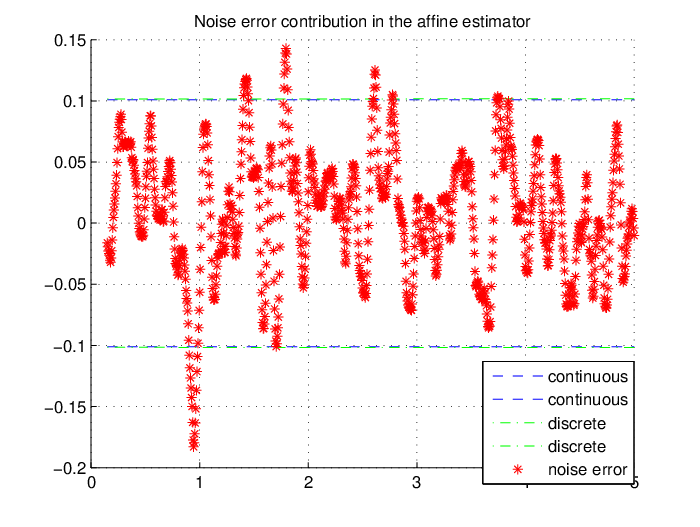
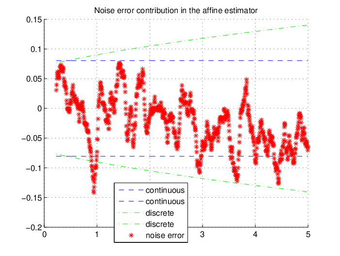
The associated noise error contributions for the estimations obtained by using respectively the affine estimator with $\kappa,\mu\in\mathbb{N}$ and the ones with $\kappa,\mu\in]-1,+\infty[$ are shown in Figure 7. In this figure, the error bounds for these noise error contributions are also shown. The dotted lines represent the error bounds obtained in the continuous case by using Theorem 4.3 with $\gamma=2$ . The dashed lines represent the error bounds obtained in this discrete case by using a discrete counter part of Theorem 4.3 with $\gamma=2$ .

In order to compare these estimations, we calculate the total error variance $\int_{0}^{5}e(\tau)^{2}d\tau$ for each estimate. As the measurement is discrete, we take $T_{s}\displaystyle\sum_{i=0}^{1000}e(\tau_{i})^{2}$ as the approximation of $\int_{0}^{5}e(\tau)^{2}d\tau$ . We also consider the $SNR$ by calculating each estimate and the associated noise error contributions. The error variance and the $SNR$ value for each estimate are given in Table 1. All the values are calculated in the same time interval $[50T_{s},5]$ . We can see that with the same $SNR$ value the estimations obtained with $\kappa,\mu\in]-1,0]$ produce smaller total errors than the ones obtained with $\kappa,\mu\in\mathbb{N}$ . Moreover, we calculate the time delay for the estimates obtained by using minimal causal estimator with $\kappa,\mu\in\mathbb{N}$ (resp. affine causal estimator with $\kappa,\mu\in\mathbb{N}$ ) which is given by $\frac{\kappa+n+1}{\kappa+\mu+2n+2}T$ (resp. $T\xi(\kappa,\mu))$ . We will make the same comparison in the next subsection.

Table 1: Error variance,

SNR

and time delay value in each estimate

$F=0.1$	$\hat{D}^{0,0}_{-18T_{s}}\dot{x}(t_{0})$	$\hat{D}^{0,-0.79}_{-30T_{s}}\dot{x}(t_{0})$
$\int_{0}^{5}e(\tau)^{2}d\tau$	$0.5506$	$0.0181$
$SNR$	$27.8019$	$27.5795$
$Theoretical\ Delay$	$0.045$	$0.0565$
$F=0.1$	$\hat{D}^{0,0}_{-30T_{s},2,0.276}\dot{x}(t_{0})$	$\hat{D}^{-0.6,-0.78}_{-46T_{s},2,0.218}\dot{x}(t_{0})$
$\int_{0}^{5}e(\tau)^{2}d\tau$	$0.5148$	$0.0197$
$SNR$	$27.6765$	$27.9936$
$Theoretical\ Delay$	$0.0414$	$0.0501$

5.2 Simulations results with a white Gaussian noise

Let $y(t_{i})=\sin(2t_{i})+C\varpi(t_{i})$ , with $t_{i}=T_{s}i$ for $i=0,\cdots,445$ ( $T_{s}=\frac{\pi}{100}$ ), be a noisy measurement of $\sin(2t_{i})$ . The samples of noise $C\varpi(t_{i})$ are simulated from a zero-mean white Gaussian $iid$ sequence where coefficient $C$ is adjusted in such a way that $SNR=20\text{dB}$ (see Figure 8).

In each figure, the solid lines represent the exact derivative of $x$ , the dashed lines represent the time-delayed estimation with $\kappa,\mu\in\mathbb{N}$ and the dotted lines represent the “delay-free” estimation with $\kappa,\mu\in]-1,0]$ . The error variance and the $SNR$ value for each estimate are given in Table 2. All the values are calculated in the same time interval $[38T_{s},14]$ .

Table 2: Error variance,

SNR

and time delay value in each estimate

$F=0.5$	$\hat{D}^{0,0}_{-25T_{s}}\dot{x}(t_{0})$	$\hat{D}^{0,-0.75}_{-25T_{s}}\dot{x}(t_{0})$
$\int_{0}^{5}e(\tau)^{2}d\tau$	$2.2351$	$0.1855$
$SNR$	$27.5396$	$27.7133$
$Theoretical\ Delay$	$0.3927$	$0.3021$
$F=0.5$	$\hat{D}^{0,0}_{-38T_{s},2,0.276}\dot{x}(t_{0})$	$\hat{D}^{-0.66,-0.7}_{-32T_{s},2,0.234}\dot{x}(t_{0})$
$\int_{0}^{5}e(\tau)^{2}d\tau$	$1.7919$	$0.0085$
$SNR$	$27.5376$	$27.2715$
$Theoretical\ Delay$	$0.3295$	$0.2352$

6 Conclusion

In this article, we study recent algebraic parametric estimation techniques introduced in [25] which provide an estimate of the derivatives by using iterated integrals of a noisy observation signal. These algebraic parametric differentiation techniques give derivative estimations which contain two sources of errors: the bias term error and the noise error contribution. In order to reduce these errors, we extend the parameter domains used in the estimators. Then, we study some error bounds which depend on these parameters. This allows us to minimize these errors. We show that a compromise choice of these parameters implies an “optimized” error among the noise error contribution, the bias term error and the time delay. We also give some examples where the errors due to numerical integration method permit us to further reduce the time delay of the estimators. We will study this interesting fact in a future work.

References

(1) Abramowitz M., Stegun I.A. (eds.): Handbook of mathematical functions. Dover Publications (1965)
(2) Al-Alaoui M.A.: A class of second-order integrators and low-pass differentiators. IEEE Trans. Circuits Syst. I 42(4), 220-223 (1995)
(3) Chen C.K., Lee J.H.: Design of high-order digital differentiators using $L_{1}$ error criteria. IEEE Trans. Circuits Syst. II 42(4), 287-291 (1995)
(4) Chitour Y.: Time-varying high-gain observers for numerical differentiation. IEEE Trans. Automat. Contr. 47, 1565-1569 (2002)
(5) Dabroom A.M., Khalil H.K.: Discrete-time implementation of high-gain observers for numerical differentiation. International Journal of Control 72, 1523-1537 (1999)
(6) Diop S., Grizzle J. W., Chaplais F.: On numerical differentiation algorithms for nonlinear estimation, in Proceedings of the IEEE Conference on Decision and Control. New York: IEEE Press 2000, Paper CD001876.
(7) Fliess M.: Analyse non standard du bruit, C.R. Acad. Sci. Paris Ser. I, 342 797-802 (2006)
(8) Fliess M.: Critique du rapport signal à bruit en théorie de l’information, Manuscript (2007) (available at http://hal.inria.fr/inria-00195987/en/)
(9) Fliess M., Join C., Mboup M., Sira-Ramírez H.: Compression différentielle de transitoires bruités. C.R. Acad. Sci., I(339):821–826, 2004. Paris.
(10) Fliess M. and Sira-Ramírez H.: Closed-loop parametric identification for continuous-time linear systems via new algebraic techniques, in H. Garnier, L. Wang (Eds): Identification of Continuous-time Models from Sampled Data, pp. 363–391, Springer (2008) (available at http://hal.inria.fr/inria-00114958/en/)
(11) Fliess M. and Sira-Ramírez H.: An algebraic framework for linear identification, ESAIM Control Optim. Calc. Variat., Vol. 9, pp. 151–168 (2003)
(12) Hào D.N., Schneider A., Reinhardt H.J.: Regularization of a non-characteristic Cauchy problem for a parabolic equation, Inverse Problems 11 (1995) 1247-1264.
(13) Haykin S., Van Veen B.: Signals and Systems, 2nd edn. John Wiley & Sons (2002)
(14) Ibrir S.: Online exact differentiation and notion of asymptotic algebraic observers. IEEE Trans. Automat. Contr. 48, 2055-2060 (2003)
(15) Ibrir S.: Linear time-derivatives trackers. Automatica 40, 397-405 (2004)
(16) Khan I.R., Ohba R.: New finite difference formulas for numerical differentiation, Journal of Computational and Applied Mathematics 126 (2000) 269-276.
(17) Levant A.: Higher-order sliding modes, differentiation and output-feedback control. International Journal of Control 76, 924-941 (2003)
(18) Lanczos C.: Applied Analysis, Prentice-Hall, Englewood Cliffs, NJ, 1956.
(19) Liu D.Y., Gibaru O., Perruquetti W.: Error analysis for a class of numerical differentiator: application to state observation, 48th IEEE Conference on Decision and Control , China, (2009) (available at http://hal.inria.fr/inria-00437129/en/)
(20) Liu D.Y., Gibaru O., Perruquetti W., Fliess M., Mboup M.: An error analysis in the algebraic estimation of a noisy sinusoidal signal. In: 16th Mediterranean conference on Control and automation (MED’ 2008), Ajaccio, (2008) (available at http://hal.inria.fr/inria-00300234/en/)
(21) Liu D.Y., Gibaru O., Perruquetti W.: Differentiation by integration with Jacobi polynomials, Journal of Computational and Applied Mathematics (2010), doi:10.1016/j.cam.2010.12.023 (available at http://hal.inria.fr/inria-00550160)
(22) Loève M.: Probability Theory, 3rd edn. D. van Nostrand Company, Inc (1963)
(23) Lyness J. N.: Finite-part integrals and the Euler-Maclaurin expansion, in Approximation and Computation, Internat. Ser. Numer. Math. 119, R. V. M. Zahar, ed., Birkhäuser Verlag, Basel, Boston, Berlin, 1994, pp. 397-407.
(24) Mboup M., Join C., Fliess M.: A revised look at numerical differentiation with an application to nonlinear feedback control. In: 15th Mediterranean conference on Control and automation (MED’07), Athenes, Greece (2007)
(25) Mboup M., Join C., Fliess M.: Numerical differentiation with annihilators in noisy environment, Numerical Algorithms 50, 4 439-467 (2009)
(26) Murio D.A.: The Mollification Method and the Numerical Solution of Ill-Posed Problems, John Wiley & Sons Inc., New York, 1993.
(27) Murio D.A., C.E. Mejía, S. Zhan: Discrete mollification and automatic numerical differentiation, Comput. Math. Appl. 35 (1998) 1-16.
(28) Nakamura G., Wang S., Wang Y.: Numerical differentiation for the second order derivatives of functions of two variables, Journal of Computational and Applied Mathematics 212 (2008) 341-358.
(29) Qu R.: A new approach to numerical differentiation and integration, Math. Comput. 24 (10) (1996) 55-68.
(30) Rader C.M., Jackson L.B.: Approximating noncausal IIR digital filters having arbitrary poles, including new Hilbert transformer designs, via forward/backward block recursion. IEEE Trans. Circuits Syst. I 53(12), 2779-2787 (2006)
(31) Ramm A.G., Smirnova A.B.: On stable numerical differentiation, Math. Comput. 70 (2001) 1131-1153.
(32) Rangarajana S.K., Purushothaman S.P.: Lanczos’ generalized derivative for higher orders, Journal of Computational and Applied Mathematics 177 (2005) 461-465.
(33) Roberts R.A., Mullis C.T.: Digital signal processing. Addison-Wesley (1987)
(34) Parzen E.: Stochastic processes, Holden-Day, San Francisco (1962)
(35) Su Y.X., Zheng C.H., Mueller P.C., Duan B.Y.: A simple improved velocity estimation for low-speed regions based on position measurements only. IEEE Trans. Control Syst. Technology 14, 937-942 (2006)
(36) Szegö G.: Orthogonal polynomials, 3rd edn. AMS, Providence, RI (1967)
(37) Wang Y., Jia X., Cheng J.: A numerical differentiation method and its application to reconstruction of discontinuity, Inverse Problems 18 (2002) 1461-1476.
(38) Wang Z., Wen R., Numerical differentiation for high orders by an integration method, Journal of Computational and Applied Mathematics 234 (2010) 941-948.
(39) Wei T., Hon Y.C., Wang Y.: Reconstruction of numerical derivatives from scattered noisy data, Inverse Problems 21 (2005) 657-672.