On the Ramified Optimal Allocation Problem Thanks: This work is supported by an NSF grant DMS-0710714.

Qinglan Xia Address: University of California at Davis
Department of Mathematics
Davis, CA, 95616 Email address: qlxia@math.ucdavis.edu URL: http://math.ucdavis.edu/˜qlxia and Shaofeng Xu Address: University of California at Davis
Department of Economics
Davis, CA, 95616 Email address: sxu@ucdavis.edu

Abstract.

This paper proposes an optimal allocation problem with ramified transport technology in a spatial economy. Ramified transportation is used to model the transport economy of scale in group transportation observed widely in both nature and efficiently designed transport systems of branching structures. The ramified allocation problem aims at finding an optimal allocation plan as well as an associated optimal allocation path to minimize overall cost of transporting commodity from factories to households. This problem differentiates itself from existing ramified transportation literature in that the distribution of production among factories is not fixed but endogenously determined as observed in many allocation practices. It’s shown that due to the transport economy of scale in ramified transportation, each optimal allocation plan corresponds equivalently to an optimal assignment map from households to factories. This optimal assignment map provides a natural partition of both households and allocation paths. We develop methods of marginal transportation analysis and projectional analysis to study properties of optimal assignment maps. These properties are then related to the search for an optimal assignment map in the context of state matrix.

Key words and phrases:

ramified transportation, transport economy of scale, optimal transport path, branching structure, allocation problem, assignment map, state matrix

2000 Mathematics Subject Classification

Primary 91B32, 58E17; Secondary 49Q20, 90B18. Journal of Economic Literature Classification. D61, C60, R12, R40.

1. Introduction

One of the lasting interests in economics is to study optimal resource allocation in a spatial economy. For instance, the well known Monge-Kantorovich transport problem aims at finding an efficient allocation plan or map for transporting some commodity from factories to households. This problem was pioneered by Monge [19] and advanced fully by Kantorovich [13] who won the Nobel prize in economics in 1975 for his seminal work on optimal allocation of resources. Recent advancement of this problem in mathematics can be found in Villani [22, 23] and references therein. Monge-Kantorovich problem has also been applied to study other related economic problems, e.g., spatial firm pricing (Buttazzo and Carlier [4]), principal-agent problem (Figalli, Kim and McCann [10]), hedonic equilibrium models (Chiappori, McCann and Nesheim [7]; Ekeland [9]), matching and partition in labor market (Carlier and Ekeland [5]; McCann and Trokhimtchouk [18]).

Recently, a new research field known as Ramified Optimal Transportation has grown out of Monge-Kantorovich problem. Representative studies can be found for instance in Gilbert [12], Xia [24, 25, 26, 27, 28, 29, 30], Maddalena, Solimini and Morel [16], Bernot, Caselles and Morel [1, 2], Brancolini, Buttazzo and Santambrogio [3], Santambrogio [21], Devillanova and Solimini [8], Xia and Vershynina [31]. Ramified optimal transport problem studies how to find an optimal transport path from sources to targets as shown in Figure 1. Different from the standard Monge-Kantorovich problem where the transportation cost is solely determined by a transport plan or map, the transportation cost in the ramified transport problem is determined by the actual transport path which transports the commodity from sources to targets. Ramified transportation indeed formally formulates the concept of transport economy of scale in group transportation observed widely in both nature (e.g. trees, blood vessels, river channel networks, lightning) and efficiently designed transport systems of branching structures (e.g. railway configurations and postage delivery networks). An application of ramified optimal transportation in economics can be found in Xia and Xu [32], which showed that a well designed ramified transport system can improve the welfare of consumers in the system.

Refer to caption — Figure 1. An optimal transport path with a ramified structure.

In this paper, we propose an optimal resource allocation problem where a planner chooses both an optimal allocation plan as well as an associated optimal transport path using ramified transport technology. In both Monge-Kantorovich and ramified transport problems, one typically assumes an exogenous fixed distribution in both sources and targets. However, in many resource allocation practices, the distribution in either sources or targets is not pre-determined but rather determined endogenously. For instance, in a production allocation problem, suppose there are $k$ factories and $\ell$ households located in different places in some area. The demand for some commodity from each household is fixed. Nevertheless, the allocation of production among factories is not pre-determined but rather depends on the distribution of demand among households as well as their relative locations to factories. A planner needs to make an efficient allocation plan of production over these $k$ factories to meet given demands from $\ell$ households. Under ramified optimal transportation, the transportation cost of each production plan is determined by an associated optimal transport path from factories to households. Consequently, the planner needs to find an optimal production plan as well as an associated optimal transport path to minimize overall cost of distributing commodity from factories to households. Another example of similar nature exists in the following storage arrangement problem. Suppose there are $k$ warehouses and $\ell$ factories located in different places in some area. Each factory has already produced some amount of commodity. However, the assignment of commodity among warehouses is not pre-determined but instead relies on the distribution of production among factories as well as relative locations between factories and warehouses. Similarly, a planner needs to make an efficient storage arrangement as well as an associated optimal transport path for storing the produced commodity in the given $k$ warehouses with minimal transportation cost.

Problem of this category is formulated as the ramified optimal allocation problem in Section 2. Throughout the following context, we will focus our discussion on the scenario of the production allocation problem. Little additional effort is needed to interpret results for other scenarios. We start with modeling a transport path from factories to households as a weighted directed graph, where the transportation cost on each edge of the graph depends linearly on the length of the edge but concavely on the amount of commodity moved on the edge. The motivation of concavity of the cost functional on quantity comes from the observation of transport economy of scale in group transportation. The more concave is the cost functional or the greater is the magnitude of transport economy of scale, the more efficient is to transport commodity in larger groups. We define the cost of an allocation plan as the minimum transportation cost of a transport path compatible with this plan. A planner needs to find an efficient allocation plan such that demands from households will be met in a least cost way. In this problem, the distribution of production over factories is not pre-determined as in Monge-Kantorovich or ramified transport problems, but endogenously determined by the distribution of demands from households as well as their relative locations to factories.

We prove the existence of the ramified allocation problem in Section 3. It’s shown that due to the transport economy of scale in ramified transportation, under any optimal allocation plan, no two factories will be connected on any associated optimal allocation path. Consequently, any optimal allocation path can be decomposed into a set of mutually disjoint transport paths originating from each factory. As a result, each household will receive her commodity from only one factory under any optimal allocation plan. It implies that each optimal allocation plan corresponds equivalently to an optimal assignment map from households to factories. Thus, solving the ramified optimal allocation problem is equivalent to finding an optimal assignment map. This optimal assignment map is shown to provide a partition not only in households but also in the associated allocation path according to the factories.

Because of the equivalence between the optimal allocation plan and assignment map, we can instead focus attention on studying the properties of optimal assignment maps in the ramified optimal allocation problem. In Section 4, we develop a method of marginal transportation analysis to study properties of optimal assignment maps. This method extends the standard marginal analysis in economics into the analysis for transport paths. It builds upon an intuitive idea that a marginal change on an optimal allocation path should not reduce the existing minimal transportation cost. Using this method, we develop a criterion which relates the optimal assignment of a household with her relative location to factories and other households, as well as her demand and productions at factories. In particular, it is shown that each factory has a nearby region such that a household living at this region will be assigned to the factory, where the size of this region depends positively on the demand of the household. In this case, the planner takes advantage of relative spatial locations between households and factories. Also, if an optimal assignment map assigns a household to some factory, then this household has a neighborhood area such that any household with a smaller demand living in this area will also be assigned to the same factory. Here, the planner utilizes the benefit in group transportation due to transport economy of scale embedded in ramified transportation. The role of spatial location and group transportation in resource allocation is further studied in Section 5 by a method of projectional analysis. We show that under an optimal assignment map, a household will be assigned to some factory only when either she lives close to the factory or she has some nearby neighbors assigned to the factory. In particular, there is an “autarky” situation when households and factories are located on two disjoint areas lying distant away from each other, the demand of households will solely be satisfied from local factories.

An important application of the properties of optimal assignment maps is that they can shed light on the search for those maps. In Section 6, we develop a search method utilizing these properties in a notion of state matrix. A state matrix represents the information set of a planner during the search process for an optimal assignment map. Any zero entry $u_{sh}$ in the matrix reflects that the planner has excluded the possibility of assigning household $h$ to factory $s$ under this map. When a state matrix has exactly one non-zero entry in each column, it completely determines an optimal assignment map by those non-zero entries. Our search method uses properties about optimal assignment maps to update some non-zero entries with zeros in a state matrix. This method is motivated by the observation that via group transportation under ramified transport technology, assignment of each household has a global effect on the allocation path as well as the associated assignment map. Thus, the planner can deduce more information about the optimal assignment map by exploiting the existing information embedded in zero entries of a state matrix. Each updated state matrix contains more zeros and thus more information than its pre-updated counterpart. This method is useful in the search for optimal assignment maps as each updating step increases the number of zero entries which in turn reduces the size of the restriction set of assignment maps in a large magnitude. In some non-trivial cases, it’s shown that this method can exactly find an optimal assignment map as desired.

2. Ramified Optimal Allocation Problem

In this section, we describe the setting of the optimal allocation model with ramified optimal transportation.

2.1. Ramified Optimal Transportation

In a spatial economy, there are $k$ factories and $\ell$ households located at $\mathbf{x}=\left\{x_{1},x_{2,\cdots,}x_{k}\right\}$ and $\left\{y_{1},y_{2},\cdots,y_{\ell}\right\}$ in some area $X$ , where $X$ is a compact convex subset of a Euclidean space $\mathbb{R}^{m}$ . In this model economy, there is only one commodity, and each household $j=1,\cdots,\ell$ has a fixed demand $n_{j}>0$ for the commodity.

For analytical convenience, we first represent households and factories as atomic Radon measures. Recall that a Radon measure $\mathbf{c}$ on $X$ is atomic if $\mathbf{c}$ is a finite sum of Dirac measures with positive multiplicities, i.e.,

\mathbf{c}=\sum\limits_{i=1}^{s}c_{i}\delta_{z_{i}}

for some integer $s\geq 1$ and some points $z_{i}\in X$ with $c_{i}>0$ for each $i=1,\cdots,s$ . The mass of $\mathbf{c}$ is denoted by

\mathfrak{m}\left(\mathbf{c}\right):=\sum_{i=1}^{s}c_{i}.

We can thus represent the $\ell$ households as an atomic measure on $X$ by

(2.1)

\mathbf{b}=\sum\limits_{j=1}^{\ell}n_{j}\delta_{y_{j}}.

For each $i=1,\cdots,k,$ denote $m_{i}$ as the units of the commodity produced at factory $i$ located at $x_{i}$ . Then, the $k$ factories can be represented by another atomic measure on $X$ by

(2.2)

\mathbf{a}=\sum_{i=1}^{k}m_{i}\delta_{x_{i}}.

In the study of transport problems, we usually assume $\mathfrak{m}\left(\mathbf{a}\right)=\mathfrak{m}\left(\mathbf{b}\right)$ , i.e.,

\sum\limits_{i=1}^{k}m_{i}=\sum\limits_{j=1}^{\ell}n_{j},

which simply means that supply equals demand in aggregate.

Next, we introduce the concept of transport path from $\mathbf{a}$ to $\mathbf{b}$ as in Xia [24].

Definition 2.1.

Suppose $\mathbf{a}$ and $\mathbf{b}$ are two atomic measures on $X$ of equal mass. A transport path from $\mathbf{a}$ to $\mathbf{b}$ is a weighted directed graph $G$ consisting of a vertex set $V\left(G\right)$ , a directed edge set $E\left(G\right)$ and a weight function $w:E\left(G\right)\rightarrow\left(0,+\infty\right)$ such that $\{x_{1},x_{2},...,x_{k}\}\cup\{y_{1},y_{2},...,y_{\ell}\}\subseteq V(G)$ and for any vertex $v\in V(G)$ , there is a balance equation

(2.3)

\sum_{e\in E(G),e^{-}=v}w(e)=\sum_{e\in E(G),e^{+}=v}w(e)+\left\{\begin{array}[]{c}m_{i},\text{\ if }v=x_{i}\text{\ for some }i=1,...,k\\ -n_{j},\text{\ if }v=y_{j}\text{\ for some }j=1,...,\ell\\ 0,\text{\ otherwise }\end{array}\right.

where each edge $e\in E\left(G\right)$ is a line segment from the starting endpoint $e^{-}$ to the ending endpoint $e^{+}$ . Denote $Path\left(\mathbf{a,b}\right)$ as the space of all transport paths from $\mathbf{a}$ to $\mathbf{b}$ .

Note that the balance equation (2.3) simply means the conservation of mass at each vertex. Viewing $G$ as an one dimensional polyhedral chain, equation (2.3) may simply be expressed as $\partial G=\mathbf{b}-\mathbf{a}$ .

Now, we consider the transportation cost of a transport path. As observed in both nature and efficiently designed transport networks, there exists a transport economy of scale underlying group transportation. For this consideration, ramified optimal transport theory uses a cost functional depending concavely on quantity and defines the transportation cost of a transport path as follows.

Definition 2.2.

For each transport path $G\in Path\left(\mathbf{a,b}\right)$ and any $\alpha\in\left[0,1\right]$ , the $\mathbf{M}_{\alpha}$ cost of $G$ is defined by

(2.4)

\mathbf{M}_{\alpha}\left(G\right):=\sum_{e\in E\left(G\right)}\left[w\left(e\right)\right]^{\alpha}length\left(e\right).

The parameter $\alpha$ represents the magnitude of transport economy of scale. The smaller the $\alpha,$ the more efficient is to move commodity in groups. Ramified optimal transport problem studies how to find a transport path to minimize the $\mathbf{M}_{\alpha}$ cost, i.e.,

(2.5)

\min_{G\in Path\left(\mathbf{a,b}\right)}\mathbf{M}_{\alpha}\left(G\right),

whose minimizer is called an optimal transport path from $\mathbf{a}$ to $\mathbf{b}$ . An optimal transport path has many nice properties. For instance, it contains no cycles by Xia [24, Proposition 2.1]. Thus, without loss of generality, we assume that all transport paths considered in the following context contain no cycles. When $\alpha<1$ , an optimal transport path is generally of branching structure. In the scenario with two sources and one target, a “Y-shaped” path is usually more preferable than a “V-shaped” path.

The following example illustrates the effect of transport economy of scale on optimal transport path in a spatial economy with one factory $\mathbf{a}=\delta_{O}$ located at origin and fifty households $\mathbf{b}=\sum_{j=1}^{50}\frac{1}{50}\delta_{y_{j}}$ of equal demand $n_{j}=\frac{1}{50}.$ The locations of these fifty households are randomly selected. As seen in Figure 2, when $\alpha=1,$ the optimal transport path is “linear” in the sense that the factory will ship commodity directly to each household. When $\alpha<1$ , the transport path becomes “ramified” as the planner would like commodity to be transported in groups in order to utilize the benefit of transport economy of scale. Furthermore, by comparing for instance the width of the transport paths for $\alpha=0.75$ and $\alpha=0.25$ , we observe that the smaller the $\alpha$ , the more likely the commodity will be transported in a large scale.

For any atomic measures $\mathbf{a}$ and $\mathbf{b}$ on $X$ of equal mass, define the minimum transportation cost as

(2.6)

d_{\alpha}\left(\mathbf{a,b}\right):=\min\left\{\mathbf{M}_{\alpha}\left(G\right):G\in Path\left(\mathbf{a,b}\right)\right\}.

As shown in Xia [24], $d_{\alpha}$ is indeed a metric on the space of atomic measures of equal mass. Also, for each $\lambda>0$ , it holds that

d_{\alpha}\left(\lambda\mathbf{a},\lambda\mathbf{b}\right)=\lambda^{\alpha}d_{\alpha}\left(\mathbf{a,b}\right).

Without loss of generality, we normalize both $\mathbf{a}$ and $\mathbf{b}$ to be a probability measure on $X$ , i.e.,

(2.7)

\sum\limits_{i=1}^{k}m_{i}=\sum\limits_{j=1}^{\ell}n_{j}=1.

2.2. Compatibility between Transport Plan and Path

For the allocation problem, a key decision a planner needs to make is about the transport plan from factories to households.

Definition 2.3.

Suppose $\mathbf{a}$ and $\mathbf{b}$ are two atomic probability measures on $X$ as in (2.2), (2.1) and (2.7). A transport plan from $\mathbf{a}$ to $\mathbf{b}$ is an atomic probability measure

(2.8)

q=\sum_{i=1}^{k}\sum_{j=1}^{\ell}q_{ij}\delta_{\left(x_{i},y_{j}\right)}

on the product space $X\times X$ such that for each $i$ and $j$ , $q_{ij}\geq 0$ ,

(2.9)

\sum_{i=1}^{k}q_{ij}=n_{j}\text{ and }\sum_{j=1}^{\ell}q_{ij}=m_{i}.

Denote $Plan\left(\mathbf{a},\mathbf{b}\right)$ as the space of all transport plans from $\mathbf{a}$ to $\mathbf{b}$ .

In a transport plan $q$ , the number $q_{ij}$ denotes the amount of commodity received by household $j$ from factory $i$ .

Now, as in Section 7.1 of Xia [24], we want to consider the compatibility between a transport path and a transport plan. Let $G$ be a given transport path in $Path\left(\mathbf{a,b}\right)$ . Since $G$ contains no cycles, for each $x_{i}$ and $y_{j}$ , there exists at most one directed polyhedral curve $g_{ij}$ on $G$ from $x_{i}$ to $y_{j}$ . In other words, there exists a list of distinct vertices

(2.10)

V\left(g_{ij}\right):=\left\{v_{i_{1}},v_{i_{2}},\cdots,v_{i_{h}}\right\}

in $V\left(G\right)$ with $x_{i}=v_{i_{1}}$ , $y_{j}=v_{i_{h}}$ , and each $\left[v_{i_{t}},v_{i_{t+1}}\right]$ is a directed edge in $E\left(G\right)$ for each $t=1,2,\cdots,h-1$ . For some pairs of $\left(i,j\right)$ , such a curve $g_{ij}$ from $x_{i}$ to $y_{j}$ may not exist, in which case we set $g_{ij}=0$ to denote the empty directed polyhedral curve. By doing so, we construct a matrix

(2.11)

g=\left(g_{ij}\right)_{k\times\ell}

with each element of $g$ being a polyhedral curve. For any transport path $G\in Path\left(\mathbf{a,b}\right)$ , such a matrix $g=\left(g_{ij}\right)$ is uniquely determined.

Definition 2.4.

Let $G\in Path\left(\mathbf{a,b}\right)$ be a transport path and $q\in Plan\left(\mathbf{a,b}\right)$ be a transport plan. The pair $\left(G,q\right)$ is compatible if $q_{ij}=0$ whenever $g_{ij}=0$ and

(2.12)

G=q\cdot g.

Here, equation (2.12) means that as polyhedral chains,

G=\sum_{i=1}^{k}\sum_{j=1}^{\ell}q_{ij}\cdot g_{ij},

where the product $q_{ij}\cdot g_{ij}$ denotes that an amount $q_{ij}$ of commodity is moved along the polyhedral curve $g_{ij}$ from factory $i$ to household $j$ .

Roughly speaking, the compatibility conditions check whether a transport plan is realizable by a transport path. Given a transport plan, the planner must design a transport path which can support this plan. To see the concept more precisely, let

\mathbf{a=}\frac{1}{4}\delta_{x_{1}}+\frac{3}{4}\delta_{x_{2}}\text{ and }\mathbf{b=}\frac{5}{8}\delta_{y_{1}}+\frac{3}{8}\delta_{y_{2}},

and consider a transport plan

(2.13)

q=\frac{1}{8}\delta_{\left(x_{1},y_{1}\right)}+\frac{1}{8}\delta_{\left(x_{1},y_{2}\right)}+\frac{1}{2}\delta_{\left(x_{2},y_{1}\right)}+\frac{1}{4}\delta_{\left(x_{2},y_{2}\right)}\in Plan\left(\mathbf{a,b}\right).

It is straight forward to see from Figure 3 that $q$ is compatible with $G_{1}$ but not $G_{2}.$ This is because there is no directed curve $g_{12}$ from factory $1$ to household $2$ in $G_{2}$ .

2.3. Ramified Allocation Problem

In the standard transport problems, e.g. Monge-Kantorovich or ramified optimal transportation, one typically assumes an exogenous fixed distribution of production among factories. In this paper, we consider a scenario where this distribution is not fixed but endogenously determined. In other words, the atomic measure $\mathbf{a}$ which represents the $k$ factories can have varying production level $m_{i}$ at each factory $i$ . This consideration is motivated by our observation that in many allocation practices as discussed in the introduction, the distribution of production among factories is not pre-determined but rather depends on the distribution of demand among households as well as their relative locations to factories.

Definition 2.5.

Let $\mathbf{x}=\left\{x_{1},x_{2,\cdots,}x_{k}\right\}$ be a finite subset of $X$ , and $\mathbf{b}$ be the atomic probability measure representing households defined in (2.1). An allocation plan from $\mathbf{x}$ to $\mathbf{b}$ is a probability measure

q=\sum_{i=1}^{k}\sum_{j=1}^{\ell}q_{ij}\delta_{\left(x_{i},y_{j}\right)}

on $X\times X$ such that $q_{ij}\geq 0$ for each $i$ , $j$ and

\sum_{i=1}^{k}q_{ij}=n_{j}\text{ for each }j=1,\cdots,\ell.

Denote $Plan\left[\mathbf{x},\mathbf{b}\right]$ as the set of all allocation plans from $\mathbf{x}$ to $\mathbf{b}$ .

Note that any allocation plan $q\in Plan\left[\mathbf{x},\mathbf{b}\right]$ corresponds to a transport plan $q$ from $\mathbf{a}\left(q\right)$ to $\mathbf{b}$ , where $\mathbf{a}\left(q\right)$ is the probability measure representing $k$ factories defined as

(2.14)

\mathbf{a}\left(q\right):=\sum_{i=1}^{k}m_{i}\left(q\right)\delta_{x_{i}},\text{ with }m_{i}\left(q\right)=\sum_{j=1}^{\ell}q_{ij},\text{ }i=1,...,k.

In other words, $Plan\left[\mathbf{x},\mathbf{b}\right]$ is the union of $Plan\left(\mathbf{a},\mathbf{b}\right)$ among all atomic probability measures $\mathbf{a}$ supported on $\mathbf{x}$ .

Example 2.1.

Any function $S:\left\{1,\cdots,\ell\right\}\rightarrow\left\{1,\cdots,k\right\}$ determines an allocation plan in $Plan\left[\mathbf{x},\mathbf{b}\right]$ as

q_{S}=\sum_{i=1}^{k}\sum_{j=1}^{\ell}q_{ij}\delta_{\left(x_{i},y_{j}\right)}\text{ with }q_{ij}=\left\{\begin{array}[]{cc}n_{j},&\text{if }i=S\left(j\right)\\ 0,&\text{else}\end{array}\right..

That is,

(2.15)

q_{S}=\sum_{j=1}^{\ell}n_{j}\delta_{\left(x_{\left(S\left(j\right)\right)},y_{j}\right)}.

For a given allocation plan, we define the associated transportation cost as follows.

Definition 2.6.

For any allocation plan $q\in Plan\left[\mathbf{x},\mathbf{b}\right]$ and $\alpha\in[0,1)$ , the ramified transportation cost of $q$ is

(2.16)

\mathbf{T}_{\alpha}\left(q\right):=\min\left\{\mathbf{M}_{\alpha}\left(G\right):G\in Path\left(\mathbf{a}\left(q\right),\mathbf{b}\right)\text{, }\left(G,q\right)\text{ compatible}\right\},

where $\mathbf{M}_{\alpha}\left(\cdot\right)$ is defined in (2.4). An allocation plan $q^{\ast}\in Plan\left[\mathbf{x},\mathbf{b}\right]$ is optimal if

\mathbf{T}_{\alpha}\left(q^{\ast}\right)\leq\mathbf{T}_{\alpha}\left(q\right)\text{ for any }q\in Plan\left[\mathbf{x},\mathbf{b}\right].

For each allocation plan $q,$ as in Xia [24, Proposition 7.3], there exists a path $G_{q}\in Path\left(\mathbf{a}\left(q\right),\mathbf{b}\right)$ such that $G_{q}$ is compatible with $q$ and

(2.17)

\mathbf{T}_{\alpha}\left(q\right)=\mathbf{M}_{\alpha}\left(G_{q}\right).

Thus, the minimum value in (2.16) is achieved by $G_{q}$ for each $q$ . Now, we are ready to define the major problem in this paper.

Problem 2.1.

(Ramified Optimal Allocation Problem) Let $X$ be a compact convex domain in $\mathbb{R}^{m}$ with the standard norm $\left\|\cdot\right\|$ . Given a finite subset $\mathbf{x}=\left\{x_{1},x_{2,\cdots,}x_{k}\right\}$ in $X$ , an atomic probability measure $\mathbf{b}$ on $X$ defined in (2.1), and a parameter $\alpha\in[0,1)$ . Find a minimizer of $\mathbf{T}_{\alpha}\left(q\right)$ among all allocation plans $q\in Plan\left[\mathbf{x},\mathbf{b}\right]$ , i.e.,

(2.18)

\min\text{ }\left\{\mathbf{T}_{\alpha}\left(q\right):q\in Plan\left[\mathbf{x},\mathbf{b}\right]\right\}.

3. Characterizing Optimal Allocation Plans

In this section, we first establish the existence result of the ramified optimal allocation problem. It’s then shown that any optimal allocation plan corresponds to an optimal assignment map from households to factories, which provides a partition in both households and transport paths.

The following proposition proves the existence of Problem 2.1.

Proposition 3.1.

The ramified optimal allocation problem (2.18) has a solution. Moreover,

(3.1)

\min\text{ }\left\{\mathbf{T}_{\alpha}\left(q\right):q\in Plan\left[\mathbf{x},\mathbf{b}\right]\right\}=\min\text{ }\left\{d_{\alpha}\left(\sum_{i=1}^{k}m_{i}\delta_{x_{i}}\mathbf{,b}\right):\vec{m}\in K\right\},

where $K=\left\{\vec{m}=\left(m_{1},...,m_{k}\right)\in\mathbb{R}_{+}^{k}:\sum_{i=1}^{k}m_{i}=1\right\}$ and $d_{\alpha}$ is defined in (2.6).

Proof.

Since $d_{\alpha}$ is a metric, it is easy to see that $d_{\alpha}\left(\sum_{i=1}^{k}m_{i}\delta_{x_{i}}\mathbf{,b}\right)$ is a continuous function in $\left(m_{1},\cdots,m_{k}\right)$ on the compact subset $K$ of $\mathbb{R}_{+}^{k}$ . Thus, the function $d_{\alpha}\left(\sum_{i=1}^{k}m_{i}\delta_{x_{i}}\mathbf{,b}\right)$ achieves its minimum value in $K$ at some $\vec{m}^{\ast}=\left(m_{1}^{\ast},...,m_{k}^{\ast}\right)$ . That is,

(3.2)

d_{\alpha}\left(\mathbf{a}^{\ast}\mathbf{,b}\right)=\min_{\vec{m}\in K}\text{ }d_{\alpha}\left(\sum_{i=1}^{k}m_{i}\delta_{x_{i}}\mathbf{,b}\right),

where $\mathbf{a}^{\ast}=\sum_{i=1}^{k}m_{i}^{\ast}\delta_{x_{i}}$ . Now, let $G^{\ast}$ be an optimal transport path in $Path\left(\mathbf{a}^{\ast}\mathbf{,b}\right)$ with $\mathbf{M}_{\alpha}\left(G^{\ast}\right)=d_{\alpha}\left(\mathbf{a}^{\ast}\mathbf{,b}\right)$ . By Xia [24, Lemma 7.1], $G^{\ast}$ has at least one compatible plan $q^{\ast}\in Plan\left(\mathbf{a}^{\ast}\mathbf{,b}\right)\subseteq Plan\left[\mathbf{x},\mathbf{b}\right]$ and thus

(3.3)

\mathbf{T}_{\alpha}\left(q^{\ast}\right)\leq\mathbf{M}_{\alpha}\left(G^{\ast}\right)=d_{\alpha}\left(\mathbf{a}^{\ast}\mathbf{,b}\right).

For any $q\in Plan\left[\mathbf{x},\mathbf{b}\right]$ , we have

$\displaystyle\mathbf{T}_{\alpha}\left(q\right)$	$\displaystyle\geq$	$\displaystyle d_{\alpha}\left(\mathbf{a}\left(q\right),\mathbf{b}\right)\text{, by (\ref{d_alpha}) and (\ref{m_alpha_q})}$
	$\displaystyle\geq$	$\displaystyle d_{\alpha}\left(\mathbf{a}^{\ast}\mathbf{,b}\right)\text{, by (\ref{d_a_min})}$
	$\displaystyle\geq$	$\displaystyle\mathbf{T}_{\alpha}\left(q^{\ast}\right)\text{, by (\ref{inequality 2}).}$

This shows that

(3.4)

\mathbf{T}_{\alpha}\left(q^{\ast}\right)=\min\text{ }\left\{\mathbf{T}_{\alpha}\left(q\right):q\in Plan\left[\mathbf{x},\mathbf{b}\right]\right\}\text{ and }\mathbf{T}_{\alpha}\left(q^{\ast}\right)=d_{\alpha}\left(\mathbf{a}^{\ast}\mathbf{,b}\right).

Thus, $q^{\ast}$ is a solution to the ramified optimal allocation problem (2.18). ∎

One implication of the above proposition is that there exists a close relationship between optimal allocation plans and underlying transport paths. To further characterize the properties of an optimal allocation plan, we introduce the concept of allocation paths as follows:

Definition 3.1.

An allocation path from $\mathbf{x}$ to $\mathbf{b}$ is a transport path $G\in Path\left(\mathbf{a,b}\right)$ for some atomic probability measure $\mathbf{a}$ supported on $\mathbf{x}$ . Denote $Path\left[\mathbf{x},\mathbf{b}\right]$ as the set of all allocation paths from $\mathbf{x}$ to $\mathbf{b}$ . An allocation path $G^{\ast}\in Path\left[\mathbf{x},\mathbf{b}\right]$ is optimal if

\mathbf{M}_{\alpha}\left(G^{\ast}\right)\leq\mathbf{M}_{\alpha}\left(G\right)\text{ for any }G\in Path\left[\mathbf{x},\mathbf{b}\right].

By the definition of $d_{\alpha}$ , equation (3.1) can be alternatively written as

(3.5)

\min\text{ }\left\{\mathbf{T}_{\alpha}\left(q\right):q\in Plan\left[\mathbf{x},\mathbf{b}\right]\right\}=\min\left\{\mathbf{M}_{\alpha}\left(G\right):G\in Path\left[\mathbf{x},\mathbf{b}\right]\right\},

which shows that the ramified optimal allocation problem corresponds to a problem of finding an optimal allocation path. The following lemma establishes the connection between optimal allocation plans and paths via the notion of compatibility.

Lemma 3.1.

Suppose $G\in Path\left[\mathbf{x},\mathbf{b}\right]$ , $q\in Plan\left[\mathbf{x},\mathbf{b}\right]$ and $\left(G,q\right)$ is compatible. Then, $G$ is an optimal allocation path if and only if $q$ is an optimal allocation plan with $\mathbf{T}_{\alpha}\left(q\right)=\mathbf{M}_{\alpha}\left(G\right)$ .

Proof.

If $G$ is an optimal allocation path, then by (3.5),

\mathbf{M}_{\alpha}\left(G\right)=\min\left\{\mathbf{T}_{\alpha}\left(\tilde{q}\right):\tilde{q}\in Plan\left[\mathbf{x},\mathbf{b}\right]\right\}.

Since $\left(G,q\right)$ is compatible, $\mathbf{T}_{\alpha}\left(q\right)\leq\mathbf{M}_{\alpha}\left(G\right)$ . Thus,

\mathbf{T}_{\alpha}\left(q\right)=\min\left\{\mathbf{T}_{\alpha}\left(\tilde{q}\right):\tilde{q}\in Plan\left[\mathbf{x},\mathbf{b}\right]\right\}=\mathbf{M}_{\alpha}\left(G\right),

and $q$ is an optimal allocation plan.

Suppose $q$ is an optimal allocation plan with $\mathbf{T}_{\alpha}\left(q\right)=\mathbf{M}_{\alpha}\left(G\right)$ , then

\mathbf{M}_{\alpha}\left(G\right)=\mathbf{T}_{\alpha}\left(q\right)=\min\left\{\mathbf{T}_{\alpha}\left(\tilde{q}\right):\tilde{q}\in Plan\left[\mathbf{x},\mathbf{b}\right]\right\}.

By (3.5), $G$ is an optimal allocation path. ∎

The next lemma presents a key property of an optimal allocation path.

Lemma 3.2.

Let $G\in Path\left[\mathbf{x},\mathbf{b}\right]$ be an optimal allocation path from $\mathbf{x}$ to $\mathbf{b}$ . Then, for any $i\neq s\in\left\{1,\cdots,k\right\}$ , $x_{i}$ and $x_{s}$ do not belong to the same connected component of $G$ .

Proof.

Assume $x_{i}$ and $x_{s}$ belong to the same connected component of an optimal allocation path $G=\left\{V\left(G\right),E\left(G\right),w:E\left(G\right)\rightarrow\left(0,+\infty\right)\right\}$ , then there exists a polyhedra curve $\gamma$ supported on $G$ from $x_{i}$ to $x_{s}$ . We may list edges of $\gamma$ as

\left\{\varepsilon_{1}e_{1},\cdots,\varepsilon_{n}e_{n}\right\}\text{ with }\varepsilon_{i}=\pm 1\text{ and }e_{i}\in E\left(G\right)\text{.}

Here, $\varepsilon_{i}=1$ (or $-1$ ) if $e_{i}$ has the same (or opposite) direction as $\gamma$ . Let

\lambda=\min_{1\leq i\leq n}w\left(e_{i}\right)>0,

and consider $G_{t}:=G+t\gamma$ for $t=\pm\lambda$ . Note that $G_{t}$ is still in $Path\left[\mathbf{x},\mathbf{b}\right]$ , and

\mathbf{M}_{\alpha}\left(G_{t}\right)-\mathbf{M}_{\alpha}\left(G\right)=\sum_{i=1}^{n}\left[\left(w\left(e_{i}\right)+t\varepsilon_{i}\right)^{\alpha}-\left(w\left(e_{i}\right)\right)^{\alpha}\right]length\left(e_{i}\right).

Thus,

			$\displaystyle\mathbf{M}_{\alpha}\left(G_{\lambda}\right)+\mathbf{M}_{\alpha}\left(G_{-\lambda}\right)-2\mathbf{M}_{\alpha}\left(G\right)$
		$\displaystyle=$	$\displaystyle\sum_{i=1}^{n}\left[\left(w\left(e_{i}\right)+\lambda\right)^{\alpha}+\left(w\left(e_{i}\right)-\lambda\right)^{\alpha}-2\left(w\left(e_{i}\right)\right)^{\alpha}\right]length\left(e_{i}\right).$

When $\alpha\in\left(0,1\right)$ , by the strict concavity of $x^{\alpha}$ , we have

\left(w\left(e_{i}\right)+\lambda\right)^{\alpha}+\left(w\left(e_{i}\right)-\lambda\right)^{\alpha}-2\left(w\left(e_{i}\right)\right)^{\alpha}<0.

When $\alpha=0$ ,

			$\displaystyle\sum_{i=1}^{n}\left[\left(w\left(e_{i}\right)+\lambda\right)^{\alpha}+\left(w\left(e_{i}\right)-\lambda\right)^{\alpha}-2\left(w\left(e_{i}\right)\right)^{\alpha}\right]length\left(e_{i}\right)$
		$\displaystyle=$	$\displaystyle-\sum\left\{length\left(e_{i}\right):w\left(e_{i}\right)=\lambda\right\}<0.$

Thus, when $\alpha\in[0,1)$ , we have

\mathbf{M}_{\alpha}\left(G_{\lambda}\right)+\mathbf{M}_{\alpha}\left(G_{-\lambda}\right)-2\mathbf{M}_{\alpha}\left(G\right)<0.

i.e.

\min\left\{\mathbf{M}_{\alpha}\left(G_{\lambda}\right),\mathbf{M}_{\alpha}\left(G_{-\lambda}\right)\right\}<\mathbf{M}_{\alpha}\left(G\right),

a contradiction with the optimality of $G$ in $Path\left[\mathbf{x},\mathbf{b}\right]$ . ∎

The above lemma says that no two factories will be connected on any optimal allocation path. Alternatively speaking, on an optimal allocation path, each single household will receive her commodity from only one factory, i.e., each household is assigned to one factory. This result is attributed to the transport economy of scale underlying ramified transportation technology. As seen in Section 2, an $\alpha\in[0,1)$ implies the existence of transport economy of scale with transporting in groups being more cost efficient than transporting separately. Any allocation path on which some single household receives commodity from two factories can not be optimal because the planner would be able to reduce transportation cost by transferring production of one factory to the other. This transfer makes the benefit of transport economy of scale more likely to be realized as commodity for this household is transported in a larger scale on the path.

The result that each household is assigned to one factory on an optimal allocation path motivates the following notion of assignment map.

Definition 3.2.

An assignment map is a function $S:\left\{1,\cdots,\ell\right\}\rightarrow\left\{1,\cdots,k\right\}$ . Let $Map\left[\ell,k\right]$ be the set of all assignment maps. For any assignment map $S\in Map\left[\ell,k\right]$ and $\alpha\in[0,1)$ , define

\mathbf{E}_{\alpha}\left(S;\mathbf{x},\mathbf{b}\right):=\sum_{i=1}^{k}d_{\alpha}\left(\mathbf{a}_{i}\mathbf{,b}_{i}\right),

where $d_{\alpha}$ is the metric defined in (2.6),

(3.6)

\mathbf{a}_{i}=\left(\sum_{j\in S^{-1}\left(i\right)}n_{j}\right)\delta_{x_{i}}\text{ and }\mathbf{b}_{i}=\sum_{j\in S^{-1}\left(i\right)}n_{j}\delta_{y_{i}}.

An assignment map $S^{\ast}\in Map\left[\ell,k\right]$ is optimal if

\mathbf{E}_{\alpha}\left(S^{\ast};\mathbf{x},\mathbf{b}\right)\leq\mathbf{E}_{\alpha}\left(S;\mathbf{x},\mathbf{b}\right)\text{ for any }S\in Map\left[\ell,k\right].

Using the concept of assignment maps, Lemma 3.2 provides a partition result for an optimal allocation path.

Proposition 3.2.

Let $G$ be an optimal allocation path from $\mathbf{x}$ to $\mathbf{b}$ . Then, there exists an assignment map $S\in Map\left[\ell,k\right]$ such that

\mathbf{E}_{\alpha}\left(S;\mathbf{x},\mathbf{b}\right)=\mathbf{M}_{\alpha}\left(G\right).

Moreover, for $\mathbf{a}_{i}$ and $\mathbf{b}_{i}$ given in (3.6), the path $G$ can be decomposed into the sum of $k$ pairwise disjoint transport paths

(3.7)

G=\sum_{i=1}^{k}G_{i}\text{ with }\mathbf{M}_{\alpha}\left(G\right)=\sum_{i=1}^{k}\mathbf{M}_{\alpha}\left(G_{i}\right),

where each $G_{i}\in Path\left(\mathbf{a}_{i},\mathbf{b}_{i}\right)$ is an optimal transport path with $\mathbf{M}_{\alpha}\left(G_{i}\right)=d_{\alpha}\left(\mathbf{a}_{i}\mathbf{,b}_{i}\right).$

Proof.

Let $G$ be an optimal allocation path from $\mathbf{x}$ to $\mathbf{b}$ . By Lemma 3.2, each $x_{i}$ determines a connected component $G_{i}$ of $G$ . Thus,

(3.8)

G=\sum_{i=1}^{k}G_{i}\text{ with }\mathbf{M}_{\alpha}\left(G\right)=\sum_{i=1}^{k}\mathbf{M}_{\alpha}\left(G_{i}\right).

For each $j\in\left\{1,\cdots,\ell\right\}$ , $y_{j}$ is clearly connected to some $x_{i}$ on $G$ . By Lemma 3.2, such an $x_{i}$ must be unique for each $j$ . Thus, we may define

S\left(j\right)=i,\text{ if }y_{j}\text{ is connected to }x_{i}\text{ on }G.

This defines an assignment map $S\in Map\left[\ell,k\right]$ . Also note that $G_{i}$ is a transport path from $\mathbf{a}_{i}$ to $\mathbf{b}_{i}$ , where $\mathbf{a}_{i},\mathbf{b}_{i}$ are given in (3.6). Since $G$ is optimal as in (3.5), each $G_{i}\in Path\left(\mathbf{a}_{i},\mathbf{b}_{i}\right)$ must also be optimal, and hence

\mathbf{M}_{\alpha}\left(G_{i}\right)=d_{\alpha}\left(\mathbf{a}_{i},\mathbf{b}_{i}\right).

Therefore,

\mathbf{M}_{\alpha}\left(G\right)=\sum_{i=1}^{k}\mathbf{M}_{\alpha}\left(G_{i}\right)=\sum_{i=1}^{k}d_{\alpha}\left(\mathbf{a}_{i},\mathbf{b}_{i}\right)=\mathbf{E}_{\alpha}\left(S;\mathbf{x},\mathbf{b}\right).

∎

Figure 4 illustrates a partition result under an optimal assignment map. This spatial economy consists of factories $\left\{x_{1},x_{2}\right\}$ and households $\left\{y_{1},\cdots,y_{145}\right\}$ with equal demand $n_{j}=\frac{1}{145}$ . The figure shows a clear partition in both the allocation path and households: First, the allocation path is decomposed into two disjoint sub-transport paths originating from factory $x_{1}$ and $x_{2}$ respectively. Second, the $145$ households are divided into two unconnected populations centered around the factory from which they receive the commodity.

Note that any assignment map $S\in Map\left[\ell,k\right]$ provides a partition among households

\mathbf{b=}\sum_{i=1}^{k}\mathbf{b}_{i},

where all households in $\mathbf{b}_{i}$ given in (3.6) are assigned to a single factory located at $x_{i}$ . For each $i$ , let $G_{i}\in Path\left(\mathbf{a}_{i}\mathbf{,b}_{i}\right)$ be an optimal transport path which transports the commodity produced at factory $i$ to households in $\mathbf{b}_{i}.$ This yields an allocation path from $\mathbf{x}$ to $\mathbf{b}$

(3.9)

G_{S}=\sum_{i=1}^{k}G_{i}\in Path\left[\mathbf{x,b}\right],

which is compatible with the allocation plan $q_{S}$ given in (2.15). Thus,

(3.10)

\mathbf{E}_{\alpha}\left(S;\mathbf{x},\mathbf{b}\right)=\sum_{i=1}^{k}d_{\alpha}\left(\mathbf{a}_{i}\mathbf{,b}_{i}\right)=\sum_{i=1}^{k}\mathbf{M}_{\alpha}\left(G_{i}\right)\geq\mathbf{M}_{\alpha}\left(G_{S}\right)\geq\mathbf{T}_{\alpha}\left(q_{S}\right).

By Proposition 3.2, any optimal allocation path is in the form of (3.9) with respect to its associated assignment map.

Now, we state the main results of this section as follows:

Theorem 1.

Given a subset $\mathbf{x}=\left\{x_{1},x_{2,\cdots,}x_{k}\right\}$ in $X$ , an atomic probability measure $\mathbf{b}$ as in (2.1), and a parameter $\alpha\in[0,1)$ .

(1)

An allocation plan $q\in Plan\left[\mathbf{x},\mathbf{b}\right]$ is optimal if and only if there exists an optimal assignment map $S\in Map\left[\ell,k\right]$ such that $q=q_{S}$ .
(2)

An allocation path $G\in Path\left[\mathbf{x},\mathbf{b}\right]$ is optimal if and only if there exists an optimal assignment map $S\in Map\left[\ell,k\right]$ such that $G=G_{S}$ for some $G_{S}$ of $S$ defined in (3.9).

(3)

Moreover,

(3.11)

\min_{q\in Plan\left[\mathbf{x},\mathbf{b}\right]}\text{ }\mathbf{T}_{\alpha}\left(q\right)=\min_{S\in Map\left[\ell,k\right]}\mathbf{E}_{\alpha}\left(S;\mathbf{x},\mathbf{b}\right)=\min_{G\in Path\left[\mathbf{x},\mathbf{b}\right]}\mathbf{M}_{\alpha}\left(G\right).

Proof.

We first show the equivalence in (1):

“ $\Longrightarrow$ ”. Suppose $q\in Plan\left[\mathbf{x},\mathbf{b}\right]$ is an optimal allocation plan. Let $G\in Path\left[\mathbf{x},\mathbf{b}\right]$ be an allocation path that is compatible with $q$ and $\mathbf{M}_{\alpha}\left(G\right)=\mathbf{T}_{\alpha}\left(q\right).$ Since $q$ is an optimal allocation plan, by Lemma 3.1, $G$ is an optimal allocation path. By Proposition 3.2, there exists an assignment map $S$ such that

(3.12)

\mathbf{E}_{\alpha}\left(S;\mathbf{x},\mathbf{b}\right)=\mathbf{M}_{\alpha}\left(G\right)=\mathbf{T}_{\alpha}\left(q\right).

Since $\left(G,q\right)$ is compatible, by (2.12), we may express

G=\sum_{i=1}^{k}\sum_{j=1}^{\ell}q_{ij}\cdot g_{ij}.

For each $j$ , by Lemma 3.2, we have $g_{sj}=0$ whenever $s\neq S\left(j\right)$ . By the compatibility of $\left(G,q\right)$ , we have $q_{sj}=0$ whenever $s\neq S\left(j\right)$ . Thus, for $i=S\left(j\right)\,$ ,

q_{ij}=\sum_{s=1}^{k}q_{sj}=n_{j}\text{, for each }j\text{.}

This shows that $q=q_{S}$ .

For any $\tilde{S}\in Map\left[\ell,k\right]$ , by (3.10) and (3.12),

\mathbf{E}_{\alpha}\left(\tilde{S};\mathbf{x},\mathbf{b}\right)\geq\mathbf{T}_{\alpha}\left(q_{\tilde{S}}\right)\geq\mathbf{T}_{\alpha}\left(q\right)=\mathbf{E}_{\alpha}\left(S;\mathbf{x},\mathbf{b}\right).

Thus, $S$ is an optimal assignment map. Since $\mathbf{E}_{\alpha}\left(S;\mathbf{x},\mathbf{b}\right)=\mathbf{T}_{\alpha}\left(q\right)$ , we have the first equality in (3.11).

“ $\Longleftarrow$ ”. Suppose $S\in Map\left[\ell,k\right]$ is an optimal assignment map. Then, by (3.10) and the first equality in (3.11),

	$\displaystyle\mathbf{T}_{\alpha}\left(q_{S}\right)$	$\displaystyle\leq$	$\displaystyle\mathbf{E}_{\alpha}\left(S;\mathbf{x},\mathbf{b}\right)=\min\left\{\mathbf{E}_{\alpha}\left(\tilde{S};\mathbf{x},\mathbf{b}\right):\tilde{S}\in Map\left[\ell,k\right]\right\}$
		$\displaystyle=$	$\displaystyle\min\text{ }\left\{\mathbf{T}_{\alpha}\left(\tilde{q}\right):\tilde{q}\in Plan\left[\mathbf{x},\mathbf{b}\right]\right\}.$

Therefore, $q_{S}\in Plan\left[\mathbf{x},\mathbf{b}\right]$ is an optimal allocation plan. This completes the proof of (1).

The second equality of (3.11) follows from the first equality of (3.11) and (3.5).

We now show the equivalence in (2):

“ $\Longleftarrow$ ” Suppose $G=G_{S}$ for some optimal assignment map $S\in Map\left[\ell,k\right]$ , then

	$\displaystyle\mathbf{M}_{\alpha}\left(G_{S}\right)$	$\displaystyle\leq$	$\displaystyle\sum_{i=1}^{k}\mathbf{M}_{\alpha}\left(G_{i}\right)=\sum_{i=1}^{k}d_{\alpha}\left(\mathbf{a}_{i}\mathbf{,b}_{i}\right)=\mathbf{E}_{\alpha}\left(S;\mathbf{x},\mathbf{b}\right)$
		$\displaystyle=$	$\displaystyle\min_{\tilde{S}\in Map\left[\ell,k\right]}\mathbf{E}_{\alpha}\left(\tilde{S};\mathbf{x},\mathbf{b}\right)=\min_{G\in Path\left[\mathbf{x},\mathbf{b}\right]}\mathbf{M}_{\alpha}\left(G\right)\text{,}$

by the optimality of $S$ and (3.11). Thus, $G=G_{S}$ is an optimal allocation path.

“ $\Longrightarrow$ ” Suppose $G\in Path\left[\mathbf{x},\mathbf{b}\right]$ is an optimal allocation path. By Proposition 3.2, $G=G_{S}$ for some $S\in Map\left[\ell,k\right]$ with $\mathbf{E}_{\alpha}\left(S;\mathbf{x},\mathbf{b}\right)=\mathbf{M}_{\alpha}\left(G\right)$ . Then, the optimality of $S$ follows from the optimality of $G$ and (3.11). ∎

Theorem 1 shows that in the ramified optimal allocation problem, there exists an equivalence between optimal allocation plan and optimal assignment map. This result has an analogous counterpart in Monge-Kantorovich problems, but has not been observed in current literature on ramified transport problems. An implication of this theorem is that one can instead search for an optimal assignment map in order to find an optimal allocation plan. Each optimal assignment map $S\in Map\left[\ell,k\right]$ would give an optimal allocation plan $q_{S}\in Plan\left[\mathbf{x},\mathbf{b}\right]$ as in (2.15). For this consideration, the rest of this paper will focus attention on characterizing the various properties of optimal assignment maps.

4. Properties of Optimal Assignment Maps via Marginal Analysis

In this section, we develop a method of marginal transportation analysis and use it to study the properties of optimal assignment maps.

We first formalize a concept of marginal transportation cost for a single-source transport system. Let $G\in Path\left(\mathfrak{m}\left(\mathbf{c}\right)\delta_{O}\mathbf{,c}\right)$ be a transport path from a single source $O$ to an atomic measure $\mathbf{c}$ of mass $\mathfrak{m}\left(\mathbf{c}\right)$ . For any point $p$ on the support of $G$ , we set

(4.1)

\theta\left(p\right):=\begin{cases}w(e),&\text{if }p\text{ is in the interior of some edge }e\in E\left(G\right)\\ \mathfrak{m}\left(\mathbf{c}\right),&\text{if }p=O\\ \sum_{e\in E(G),e^{+}=p}w(e),&\text{if }p\in V\left(G\right)\setminus\left\{O\right\}\end{cases},

which represents the mass flowing through $p$ , where $e^{+}$ denotes the ending endpoint of edge $e\in E\left(G\right)$ . Since $G$ has a single source and contains no cycles, for any point $p$ on $G$ , there exists a unique polyhedral curve $\gamma_{p}$ on $G$ from $O$ to $p$ . Moreover, for any point $s\in\gamma_{p}$ , it holds that

(4.2)

\mathfrak{m}\left(\mathbf{c}\right)\geq\theta\left(s\right)\geq\theta\left(p\right)\text{.}

When the mass at $p$ changes by an amount $\Delta m$ with $\Delta m\geq-$ $\mathbf{\theta}\left(p\right)$ , then the mass flowing through each point of $\gamma_{p}$ also changes by $\Delta m$ . As a result, the corresponding increment of the transportation cost is

(4.3)		$\displaystyle\Delta C_{G}\left(p,\Delta m\right):$	$\displaystyle=$	$\displaystyle\mathbf{M}_{\alpha}\left(G+\left(\Delta m\right)\gamma_{p}\right)-\mathbf{M}_{\alpha}\left(G\right)$
(4.3)			$\displaystyle=$	$\displaystyle\int_{\gamma_{p}}\left(\theta\left(s\right)+\Delta m\right)^{\alpha}-\left(\theta\left(s\right)\right)^{\alpha}ds.$

The marginal transportation cost at $p$ via $G$ is defined by

MC_{G}\left(p\right):=\lim_{\Delta m\rightarrow 0}\frac{\Delta C_{G}\left(p,\Delta m\right)}{\Delta m}=\alpha\int_{\gamma_{p}}\left(\theta\left(s\right)\right)^{\alpha-1}ds.

The following proposition establishes some properties of the function $\Delta C_{G}\left(p,\Delta m\right)$ . Those properties are the key elements of marginal transportation analysis used to study optimal assignment maps later.

Proposition 4.1.

For any $G\in Path\left(\mathfrak{m}\left(\mathbf{c}\right)\delta_{O}\mathbf{,c}\right)$ and $p$ on $G$ , we have

(4.4)

\Delta C_{G}\left(p,-\Delta m\right)=-\Delta C_{\tilde{G}}\left(p,\Delta m\right),\text{ for }\Delta m\in\left[-\theta\left(p\right),\theta\left(p\right)\right],

where $\tilde{G}=G-\left(\Delta m\right)\gamma_{p}$ . Moreover, for any $\Delta m\geq 0$ , we have

(4.5)

\left[\left(\mathfrak{m}\left(\mathbf{c}\right)+\Delta m\right)^{\alpha}-\mathfrak{m}\left(\mathbf{c}\right)^{\alpha}\right]\int_{\gamma_{p}}ds\leq\Delta C_{G}\left(p,\Delta m\right)\leq\left[\left(\theta\left(p\right)+\Delta m\right)^{\alpha}-\theta\left(p\right)^{\alpha}\right]\int_{\gamma_{p}}ds.

If, in addition, $G\in Path\left(\mathfrak{m}\left(\mathbf{c}\right)\delta_{O}\mathbf{,c}\right)$ is optimal in (2.5), then

(4.6)

d_{\alpha}\left(\left(\mathfrak{m}\left(\mathbf{c}\right)+\Delta m\right)\delta_{O},\mathbf{c+}\left(\Delta m\right)\delta_{p}\right)-d_{\alpha}\left(\mathfrak{m}\left(\mathbf{c}\right)\delta_{O},\mathbf{c}\right)\leq\Delta C_{G}\left(p,\Delta m\right)

for any $\Delta m\geq-$ $\mathbf{\theta}\left(p\right)$ with $p$ on $G$ .

Proof.

Let $\tilde{G}=G-\left(\Delta m\right)\gamma_{p}$ , then when $\Delta m\in\left[-\theta\left(p\right),\theta\left(p\right)\right]$ ,

$\displaystyle\Delta C_{G}\left(p,-\Delta m\right)$	$\displaystyle=$	$\displaystyle\int_{\gamma_{p}}\left(\theta\left(s\right)-\Delta m\right)^{\alpha}-\left(\theta\left(s\right)\right)^{\alpha}ds$
	$\displaystyle=$	$\displaystyle-\int_{\gamma_{p}}\left[\left(\left(\theta\left(s\right)-\Delta m\right)+\Delta m\right)^{\alpha}-\left(\theta\left(s\right)-\Delta m\right)^{\alpha}\right]ds$
	$\displaystyle=$	$\displaystyle-\Delta C_{\tilde{G}}\left(p,\Delta m\right).$

For any $\Delta m\geq 0$ , note that the function $f\left(t\right):=\left(t+\Delta m\right)^{\alpha}-t^{\alpha}$ is monotonic non-increasing on $t>0$ when $0\leq\alpha<1$ . By (4.2), we have

\left(\mathfrak{m}\left(\mathbf{c}\right)+\Delta m\right)^{\alpha}-\left(\mathfrak{m}\left(\mathbf{c}\right)\right)^{\alpha}\leq\left(\theta\left(s\right)+\Delta m\right)^{\alpha}-\left(\theta\left(s\right)\right)^{\alpha}\leq\left(\theta\left(p\right)+\Delta m\right)^{\alpha}-\left(\theta\left(p\right)\right)^{\alpha}.

Thus, by (4.3), inequalities (4.5) hold.

When $G$ is also optimal, we have $\mathbf{M}_{\alpha}\left(G\right)=d_{\alpha}\left(\mathfrak{m}\left(\mathbf{c}\right)\delta_{O},\mathbf{c}\right)$ . For any $\Delta m\geq-$ $\mathbf{\theta}\left(p\right)$ , since $G+\left(\Delta m\right)\gamma_{p}\in Path\left(\left(\mathfrak{m}\left(\mathbf{c}\right)+\Delta m\right)\delta_{O},\mathbf{c+}\left(\Delta m\right)\delta_{p}\right)$ , we have

	$\displaystyle\Delta C_{G}\left(p,\Delta m\right)$	$\displaystyle=$	$\displaystyle\mathbf{M}_{\alpha}\left(G+\left(\Delta m\right)\gamma_{p}\right)-\mathbf{M}_{\alpha}\left(G\right)$
		$\displaystyle\geq$	$\displaystyle d_{\alpha}\left(\left(\mathfrak{m}\left(\mathbf{c}\right)+\Delta m\right)\delta_{O},\mathbf{c+}\left(\Delta m\right)\delta_{p}\right)-d_{\alpha}\left(\mathfrak{m}\left(\mathbf{c}\right)\delta_{O},\mathbf{c}\right).$

∎

Now, we apply marginal transportation analysis developed above to study properties of an optimal assignment map. Let $G\in Path\left[\mathbf{x},\mathbf{b}\right]$ be any optimal allocation path. By Theorem 1, $G$ must be in the form of (3.9), which is simply a disjoint union of single-source paths $G_{i}$ ’s. For any $p$ on $G$ , there exists a unique $i$ such that $p$ is on $G_{i}$ . Thus, we can define the corresponding $\theta_{i}\left(p\right)$ and $\Delta C_{G_{i}}\left(p,\Delta m\right)$ as in (4.1) and (4.3). Then, we set

\theta\left(p\right):=\theta_{i}\left(p\right)\text{ and }\Delta C_{G}\left(p,\Delta m\right):=\Delta C_{G_{i}}\left(p,\Delta m\right)

for any $p$ on the support of $G$ .

For any $\alpha\in(0,1)$ and $\sigma\geq\epsilon>0$ , define

(4.7)

\rho_{\alpha}\left(\sigma,\epsilon\right):=\left(\frac{\sigma}{\epsilon}\right)^{\alpha}-\left(\frac{\sigma}{\epsilon}-1\right)^{\alpha}\text{.}

The function $\rho_{\alpha}\left(\sigma,\varepsilon\right)$ is decreasing in $\sigma$ and increasing in $\epsilon$ ; also $0<\rho_{\alpha}\left(\sigma,\epsilon\right)\leq 1$ for any $\sigma\geq\epsilon>0$ . For $\alpha=0$ , set $\rho_{0}\left(\sigma,\epsilon\right)=0$ when $\sigma>\epsilon>0$ and $\rho_{0}\left(\sigma,\epsilon\right)=1$ when $\sigma=\epsilon>0$ .

Proposition 4.2.

Suppose $G\in Path\left[\mathbf{x},\mathbf{b}\right]$ is an optimal allocation path as given in (3.7). Let $p$ be a point on $G_{s}$ for some $s\in\left\{1,\cdots,k\right\}$ and $\Delta m\in(0,\theta\left(p\right)]$ . For any $p^{\ast}$ on $G$ with $\gamma_{p}\cap\gamma_{p^{\ast}}$ having zero length, we have

(4.8)

\Delta C_{G}\left(p,-\Delta m\right)+\left(\Delta m\right)^{\alpha}\left\|p-p^{\ast}\right\|+\Delta C_{G}\left(p^{\ast},\Delta m\right)\geq 0

and

(4.9)

\left\|p-p^{\ast}\right\|+\rho_{\alpha}\left(\theta\left(p^{\ast}\right)+\Delta m,\Delta m\right)\int_{\gamma_{p^{\ast}}}ds\geq\rho_{\alpha}\left(\mathfrak{m}\left(\mathbf{b}_{s}\right),\Delta m\right)\int_{\gamma_{p}}ds,

where $\left\|\cdot\right\|$ stands for the standard norm on $\mathbb{R}^{m}$ . In particular, for any $i\in\left\{1,\cdots,k\right\}$ ,

(4.10)

\left\|p-x_{i}\right\|\geq\rho_{\alpha}\left(\mathfrak{m}\left(\mathbf{b}_{s}\right),\Delta m\right)\int_{\gamma_{p}}ds\geq\rho_{\alpha}\left(\mathfrak{m}\left(\mathbf{b}_{s}\right),\Delta m\right)\left\|p-x_{s}\right\|.

Moreover, suppose $p^{\ast}$ is on $G_{i}$ with $i\neq s$ and $\Delta m\leq\theta\left(p^{\ast}\right)$ , then

(4.11)

\left\|p-p^{\ast}\right\|+\frac{\rho_{\alpha}\left(\theta\left(p^{\ast}\right)+\Delta m,\Delta m\right)}{\rho_{\alpha}\left(\mathfrak{m}\left(\mathbf{b}_{i}\right),\Delta m\right)}\left\|p^{\ast}-x_{i}\right\|\geq\rho_{\alpha}\left(\mathfrak{m}\left(\mathbf{b}_{s}\right),\Delta m\right)\left\|p-x_{s}\right\|.

Proof.

Let $\hat{G}=G-\left(\Delta m\right)\gamma_{p}+\left(\Delta m\right)[p,p^{\ast}]+\left(\Delta m\right)\gamma_{p^{\ast}}$ , where $[p,p^{\ast}]$ denotes the line segment from $p$ to $p^{\ast}$ . Then, when the intersection of polyhedral curves $\gamma_{p}\cap\gamma_{p^{\ast}}$ has length zero, we have

			$\displaystyle\Delta C_{G}\left(p,-\Delta m\right)+\left(\Delta m\right)^{\alpha}\left\\|p-p^{\ast}\right\\|+\Delta C_{G}\left(p^{\ast},\Delta m\right)$
		$\displaystyle=$	$\displaystyle\int_{\gamma_{p}}\left[\left(\theta\left(s\right)-\Delta m\right)^{\alpha}-\theta\left(s\right)^{\alpha}\right]ds+\left(\Delta m\right)^{\alpha}\left\\|p-p^{\ast}\right\\|$
			$\displaystyle+\int_{\gamma_{p^{\ast}}}\left[\left(\theta\left(s\right)+\Delta m\right)^{\alpha}-\theta\left(s\right)^{\alpha}\right]ds$
		$\displaystyle\geq$	$\displaystyle\mathbf{M}_{\alpha}\left(\hat{G}\right)-\mathbf{M}_{\alpha}\left(G\right)\geq 0\text{, by the optimality of }G.$

To prove (4.9), we observe that

			$\displaystyle\left(\Delta m\right)^{\alpha}\left[\left\\|p-p^{\ast}\right\\|+\rho_{\alpha}\left(\theta\left(p^{\ast}\right)+\Delta m,\Delta m\right)\int_{\gamma_{p^{\ast}}}ds\right]$
		$\displaystyle=$	$\displaystyle\left(\Delta m\right)^{\alpha}\left\\|p-p^{\ast}\right\\|+\left[\left(\theta\left(p^{\ast}\right)+\Delta m\right)^{\alpha}-\left(\theta\left(p^{\ast}\right)\right)^{\alpha}\right]\int_{\gamma_{p^{\ast}}}ds$
		$\displaystyle\geq$	$\displaystyle\left(\Delta m\right)^{\alpha}\left\\|p-p^{\ast}\right\\|+\Delta C_{G}\left(p^{\ast},\Delta m\right)\text{, by (\ref{incrementcost_comparison})}$
		$\displaystyle\geq$	$\displaystyle-\Delta C_{G}\left(p,-\Delta m\right)\text{, by (\ref{increment_cost_inequality})}$
		$\displaystyle=$	$\displaystyle\Delta C_{\tilde{G}}\left(p,\Delta m\right)\text{, by (\ref{alternative})}$
		$\displaystyle\geq$	$\displaystyle\left[\left(\mathfrak{m}\left(\mathbf{b}_{s}\right)\right)^{\alpha}-\left(\mathfrak{m}\left(\mathbf{b}_{s}\right)-\Delta m\right)^{\alpha}\right]\int_{\gamma_{p}}ds\text{, by (\ref{incrementcost_comparison})}$
		$\displaystyle=$	$\displaystyle\left(\Delta m\right)^{\alpha}\rho_{\alpha}\left(\mathfrak{m}\left(\mathbf{b}_{s}\right),\Delta m\right)\int_{\gamma_{p}}ds\geq\left(\Delta m\right)^{\alpha}\rho_{\alpha}\left(\mathfrak{m}\left(\mathbf{b}_{s}\right),\Delta m\right)\left\\|p-x_{s}\right\\|\text{.}$

In particular, when $p^{\ast}=x_{i}$ for some $i$ , (4.9) becomes (4.10) as $\int_{\gamma_{p^{\ast}}}ds=0$ .

Now, suppose $p^{\ast}$ is on $G_{i}$ with $i\neq s$ . Apply (4.10) to $p^{\ast}$ , we have

\frac{\left\|p^{\ast}-x_{i}\right\|}{\rho_{\alpha}\left(\mathfrak{m}\left(\mathbf{b}_{i}\right),\Delta m\right)}\geq\int_{\gamma_{p^{\ast}}}ds.

Therefore,

			$\displaystyle\left\\|p-p^{\ast}\right\\|+\frac{\rho_{\alpha}\left(\theta\left(p^{\ast}\right)+\Delta m,\Delta m\right)}{\rho_{\alpha}\left(\mathfrak{m}\left(\mathbf{b}_{i}\right),\Delta m\right)}\left\\|p^{\ast}-x_{i}\right\\|$
		$\displaystyle\geq$	$\displaystyle\left\\|p-p^{\ast}\right\\|+\rho_{\alpha}\left(\theta\left(p^{\ast}\right)+\Delta m,\Delta m\right)\int_{\gamma_{p^{\ast}}}ds$
		$\displaystyle\geq$	$\displaystyle\rho_{\alpha}\left(\mathfrak{m}\left(\mathbf{b}_{s}\right),\Delta m\right)\int_{\gamma_{p}}ds\text{, by (\ref{p_p*})}$
		$\displaystyle\geq$	$\displaystyle\rho_{\alpha}\left(\mathfrak{m}\left(\mathbf{b}_{s}\right),\Delta m\right)\left\\|p-x_{s}\right\\|\text{.}$

∎

Proposition 4.2 rests on the key inequality (4.8), which follows intuitively by standard marginal argument. For convenience of illustration, let $p$ denote the location $y_{j}$ of household $j$ who is connected to factory $s$ by some curve $\gamma_{p}.$ A planner will find it not optimal to choose an allocation path $G$ such that $\Delta C_{G}\left(y_{j},-\Delta m\right)+\left(\Delta m\right)^{\alpha}\left\|y_{j}-p^{\ast}\right\|+\Delta C_{G}\left(p^{\ast},\Delta m\right)<0$ for $p^{\ast}$ on some $G_{i}.$ It is because in this case the planner has a less costly alternative by transferring $\Delta m$ amount of production from factory $s$ to factory $i$ and transporting this additional $\Delta m$ units of commodity from factory $i$ first to a stopover point $p^{\ast}$ via curve $\gamma_{p^{\ast}}$ and then directly from $p^{\ast}$ to household $j$ . It’s clear that this strategy will send the same amount of commodity to household $j$ as before. However, by the inequality, the reduction in transportation cost $-\Delta C_{G}\left(p,-\Delta m\right)$ on curve $\gamma_{p}$ exceeds its increase counterpart $\Delta C_{G}\left(p^{\ast},\Delta m\right)+\left(\Delta m\right)^{\alpha}\left\|y_{j}-p^{\ast}\right\|,$ which cannot be the case for an optimal allocation path.

By means of this proposition, we easily obtain the following results regarding the properties of optimal assignment maps.

Theorem 2.

Suppose $S\in Map\left[\ell,k\right]$ is an optimal assignment map. Let $j\in\left\{1,\cdots,\ell\right\}$ and $s\in\left\{1,\cdots,k\right\}$ . If

(4.12)

y_{j}\in\digamma_{S}^{s}\left(n_{j}\right):=\left\{z\in\mathbb{R}^{m}:\min_{i\neq s}\left\|z-x_{i}\right\|<\rho_{\alpha}\left(\mathfrak{m}\left(\mathbf{b}_{s}\right),n_{j}\right)\left\|z-x_{s}\right\|\right\},

then $S\left(j\right)\neq s$ . If

(4.13)

y_{j}\in\Omega_{S}^{s}\left(n_{j}\right):=\left\{z\in\mathbb{R}^{m}:\left\|z-x_{s}\right\|<\min_{i\neq s}\rho_{\alpha}\left(\mathfrak{m}\left(\mathbf{b}_{i}\right),n_{j}\right)\left\|z-x_{i}\right\|\right\},

then $S\left(j\right)=s$ .

Proof.

Assume $y_{j}\in\digamma_{S}^{s}\left(n_{j}\right)$ but $S\left(j\right)=s$ . Let $G=G_{S}$ be an allocation path as in (3.9). By Theorem 1, $G\in Path\left[\mathbf{x},\mathbf{b}\right]$ is an optimal allocation path. Clearly, $y_{j}$ is on $G_{s}$ when $S\left(j\right)=s\,$ . Apply (4.10) to $p=y_{j}$ and $\Delta m=n_{j}$ , we have

\min_{i\in\left\{1,\cdots,k\right\}}\left\|y_{j}-x_{i}\right\|\geq\rho_{\alpha}\left(\mathfrak{m}\left(\mathbf{b}_{s}\right),n_{j}\right)\left\|y_{j}-x_{s}\right\|,

which contradicts (4.12).

On the other hand, for each $i\neq s$ , if $y_{j}\in\Omega_{S}^{s}\left(n_{j}\right)$ , then

\min_{i^{\ast}\neq i}\left\|y_{j}-x_{i^{\ast}}\right\|\leq\left\|y_{j}-x_{s}\right\|<\rho_{\alpha}\left(\mathfrak{m}\left(\mathbf{b}_{i}\right),n_{j}\right)\left\|y_{j}-x_{i}\right\|.

By (4.12), $y_{j}\in\digamma_{S}^{i}\left(n_{j}\right)$ and $S\left(j\right)\neq i$ for such $i\neq s$ . Thus, $S\left(j\right)=s$ . ∎

Intuitively speaking, inequality (4.12) says that if household $j$ locates “closer” to some factory than factory $s$ , then the planner will not assign her to the factory $s$ . Here the relative closeness is weighted by a number $\rho_{\alpha}\left(\mathfrak{m}\left(\mathbf{b}_{s}\right),n_{j}\right)$ . When the production $\mathfrak{m}\left(\mathbf{b}_{s}\right)$ at factory $s$ is low, due to the transport economy of scale, one would expect that the planner would less likely assign household $j$ to factory $s$ . This predication is justified by Theorem 2 because in this case, inequality (4.12) becomes more likely to hold as $\rho_{\alpha}\left(\mathfrak{m}\left(\mathbf{b}_{s}\right),n_{j}\right)$ is high. The later part (4.13) of the theorem states a special case that if household $j$ is located uniformly closer to a factory $s$ than to other factories, then she will be assigned to factory $s$ under any optimal assignment map.

We now give a geometric description of the sets $\digamma_{S}^{s}\left(n_{j}\right)$ and $\Omega_{S}^{s}\left(n_{j}\right)$ .

Lemma 4.1.

For any constant $C\in\left(0,1\right)$ , the set

\left\{x\in\mathbb{R}^{m}:\left\|x-x_{i}\right\|<C\left\|x-x_{s}\right\|\right\}=B\left(x_{i}+\frac{C^{2}}{1-C^{2}}\left(x_{i}-x_{s}\right),\frac{C}{1-C^{2}}\left\|x_{i}-x_{s}\right\|\right),

where $B\left(x,r\right)$ denotes the open ball $\left\{z\in\mathbb{R}^{m}:\left\|z-x\right\|<r\right\}$ .

Proof.

Indeed,

			$\displaystyle\left\\|x-x_{i}\right\\|<C\left\\|x-x_{s}\right\\|$
		$\displaystyle\iff$	$\displaystyle\left\\|x-x_{i}\right\\|^{2}<C^{2}\left\\|x-x_{s}\right\\|^{2}$
		$\displaystyle\iff$	$\displaystyle\left\\|x\right\\|^{2}-2x\cdot x_{i}+\left\\|x_{i}\right\\|^{2}<C^{2}\left(\left\\|x\right\\|^{2}-2x\cdot x_{s}+\left\\|x_{s}\right\\|^{2}\right)$
		$\displaystyle\iff$	$\displaystyle\left\\|x\right\\|^{2}-2x\cdot\frac{x_{i}-C^{2}x_{s}}{1-C^{2}}<\frac{C^{2}\left\\|x_{s}\right\\|^{2}-\left\\|x_{i}\right\\|^{2}}{1-C^{2}}$
		$\displaystyle\iff$	$\displaystyle\left\\|x-x_{i}-\frac{C^{2}}{1-C^{2}}\left(x_{i}-x_{s}\right)\right\\|^{2}<\frac{C^{2}}{\left(1-C^{2}\right)^{2}}\left\\|x_{i}-x_{s}\right\\|^{2}.$

∎

Clearly, the ball $B\left(x_{i}+\frac{C^{2}}{1-C^{2}}\left(x_{i}-x_{s}\right),\frac{C}{1-C^{2}}\left\|x_{i}-x_{s}\right\|\right)$ given above contains $x_{i}$ but not $x_{s}$ . By Lemma 4.1, (4.12) says that geometrically, if household $j$ lies in the union of $k-1$ open balls

\digamma_{S}^{s}\left(n_{j}\right)=\bigcup_{i\neq s}B\left(x_{i}+\frac{\left(w_{sj}\right)^{2}}{1-\left(w_{sj}\right)^{2}}\left(x_{i}-x_{s}\right),\frac{w_{sj}}{1-\left(w_{sj}\right)^{2}}\left\|x_{s}-x_{i}\right\|\right),

where $w_{sj}=\rho_{\alpha}\left(\mathfrak{m}\left(\mathbf{b}_{s}\right),n_{j}\right)$ , then $S\left(j\right)\neq s$ . Also, (4.13) says that if the household $j$ lies in the intersection of $\left(k-1\right)$ balls

(4.14)

\Omega_{S}^{s}\left(n_{j}\right)=\bigcap_{i\neq s}B\left(x_{s}+\frac{\left(w_{ij}\right)^{2}}{1-\left(w_{ij}\right)^{2}}\left(x_{s}-x_{i}\right),\frac{w_{ij}}{1-\left(w_{ij}\right)^{2}}\left\|x_{i}-x_{s}\right\|\right)

for some $s$ , then $S\left(j\right)=s$ .

Since $\mathfrak{m}\left(\mathbf{b}_{s}\right)\leq\mathfrak{m}\left(\mathbf{b}\right)=1$ and the function $\rho_{\alpha}\left(\cdot,n_{j}\right)$ is decreasing, we have $\rho_{\alpha}\left(1,n_{j}\right)\leq\rho_{\alpha}\left(\mathfrak{m}\left(\mathbf{b}_{s}\right),n_{j}\right)$ and thus

(4.15)		$\displaystyle\digamma^{s}\left(n_{j}\right)$	$\displaystyle:$	$\displaystyle=\left\{z:\min_{i\neq s}\left\\|z-x_{i}\right\\|<\rho_{\alpha}(1,n_{j})\left\\|z-x_{s}\right\\|\right\}\subseteq\digamma_{S}^{s}\left(n_{j}\right)\text{,}$
(4.16)		$\displaystyle\Omega^{s}\left(n_{j}\right)$	$\displaystyle:$	$\displaystyle=\left\{z:\left\\|z-x_{s}\right\\|<\rho_{\alpha}\left(1,n_{j}\right)\min_{s\neq i}\left\\|z-x_{i}\right\\|\right\}\subseteq\Omega_{S}^{s}\left(n_{j}\right)$

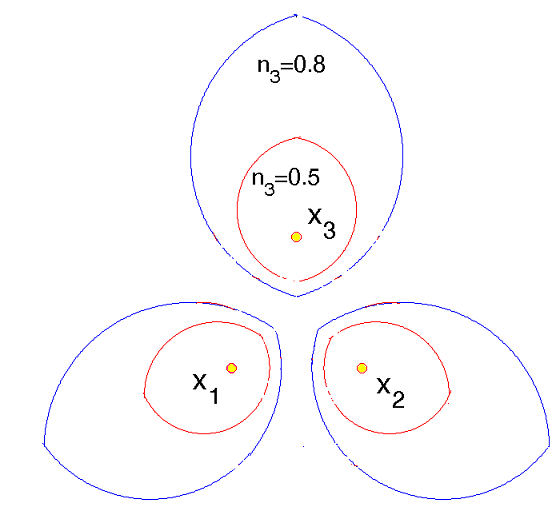
for any optimal assignment map $S$ . Note that the set $\digamma^{s}\left(n_{j}\right)$ (or $\Omega^{s}\left(n_{j}\right)$ ) is still the union (or intersection) of $k-1$ balls in $\mathbb{R}^{m}$ , and is independent of $S$ . For example, the sets $\Omega^{s}\left(n_{j}\right)$ with $n_{j}=0.8$ and $n_{j}=0.5$ are given by Figure 5, where $x_{1}=(0,0),x_{2}=(2,0)$ and $x_{3}=(1,2)$ .

Corollary 4.1.

For any optimal assignment map $S\in Map\left[\ell,k\right]$ and $s\in\left\{1,\cdots,k\right\}$ , if $y_{j}\in\digamma^{s}\left(n_{j}\right)$ , then $S\left(j\right)\neq s$ . If $y_{j}\in\Omega^{s}\left(n_{j}\right)$ , then $S\left(j\right)=s$ .

Proof.

It follows from Theorem 2, (4.15) and (4.16). ∎

This corollary shows that if the household $j$ falls into the region $\Omega^{s}\left(n_{j}\right)$ of some factory $s,$ then she will be assigned to this factory under any optimal assignment map $S$ . As a result, if all households belong to the union of regions $\Omega^{s}\left(n_{j}\right)$ of factories $s$ except factory $i$ , then factory $i$ will not be used. Note that as $\rho_{\alpha}\left(1,n_{j}\right)$ is increasing in $n_{j},$ the size of the region $\Omega^{s}\left(n_{j}\right)$ increases with $n_{j}$ as shown in Figure 5.

Theorem 3.

Suppose $S\in Map\left[\ell,k\right]$ is an optimal assignment map, $h$ and $j\in\left\{1,\cdots,\ell\right\}$ with $n_{j}\leq n_{h}$ . If $S\left(h\right)=s^{\ast}\neq s$ for some $s\in\left\{1,\cdots,k\right\}$ and

(4.17)

y_{j}\in\digamma_{S}^{s,h}\left(n_{j}\right):=\left\{z\in\mathbb{R}^{m}\left|\begin{array}[]{l}\left\|z-y_{h}\right\|+\frac{\rho_{\alpha}\left(n_{h}+n_{j},n_{j}\right)}{\rho_{\alpha}\left(\mathfrak{m}\left(\mathbf{b}_{s^{\ast}}\right),n_{j}\right)}\left\|y_{h}-x_{s^{\ast}}\right\|\\ <\rho_{\alpha}\left(\mathfrak{m}\left(\mathbf{b}_{s}\right),n_{j}\right)\left\|z-x_{s}\right\|\end{array}\right\}\right.,

then $S\left(j\right)\neq s$ . If $S\left(h\right)=s$ for some $s\in\left\{1,\cdots,k\right\}$ and

(4.18)

y_{j}\in\Omega_{S}^{s,h}\left(n_{j}\right):=\bigcap_{i\neq s,\mathfrak{m}\left(\mathbf{b}_{i}\right)\geq n_{j}}\left\{z\in\mathbb{R}^{m}\left|\begin{array}[]{l}\left\|z-y_{h}\right\|+\frac{\rho_{\alpha}\left(n_{h}+n_{j},n_{j}\right)}{\rho_{\alpha}\left(\mathfrak{m}\left(\mathbf{b}_{s}\right),n_{j}\right)}\left\|y_{h}-x_{s}\right\|\\ <\rho_{\alpha}\left(\mathfrak{m}\left(\mathbf{b}_{i}\right),n_{j}\right)\left\|z-x_{i}\right\|\end{array}\right\}\right.,

then $S\left(j\right)=s$ .

Proof.

In the first scenario, assume $S\left(h\right)=s^{\ast}\neq s$ , $y_{j}\in\digamma_{S}^{s,h}\left(n_{j}\right)$ but $S\left(j\right)=s$ . Then

			$\displaystyle\left\\|y_{j}-y_{h}\right\\|+\frac{\rho_{\alpha}\left(n_{h}+n_{j},n_{j}\right)}{\rho_{\alpha}\left(\mathfrak{m}\left(\mathbf{b}_{s^{\ast}}\right),n_{j}\right)}\left\\|y_{h}-x_{s^{\ast}}\right\\|$
		$\displaystyle\geq$	$\displaystyle\left\\|y_{j}-y_{h}\right\\|+\frac{\rho_{\alpha}\left(\theta\left(y_{h}\right)+n_{j},n_{j}\right)}{\rho_{\alpha}\left(\mathfrak{m}\left(\mathbf{b}_{s^{\ast}}\right),n_{j}\right)}\left\\|y_{h}-x_{s^{\ast}}\right\\|\text{ as }\theta\left(y_{h}\right)\geq n_{h}\text{,}$
		$\displaystyle\geq$	$\displaystyle\rho_{\alpha}\left(\mathfrak{m}\left(\mathbf{b}_{s}\right),n_{j}\right)\left\\|y_{j}-x_{s}\right\\|\text{, by (\ref{p_neighborhood}),}$

a contradiction with $y_{j}\in\digamma_{S}^{s,h}\left(n_{j}\right)$ . Thus, $S\left(j\right)\neq s.$

Now, in the second scenario, assume $S\left(h\right)=s$ , $y_{j}\in\Omega_{S}^{s,h}\left(n_{j}\right)$ but $S\left(j\right)=i^{\ast}$ for some $i^{\ast}\neq s$ . Then,

			$\displaystyle\left\\|y_{j}-y_{h}\right\\|+\frac{\rho_{\alpha}\left(n_{h}+n_{j},n_{j}\right)}{\rho_{\alpha}\left(\mathfrak{m}\left(\mathbf{b}_{s}\right),n_{j}\right)}\left\\|y_{h}-x_{s}\right\\|$
		$\displaystyle\geq$	$\displaystyle\left\\|y_{j}-y_{h}\right\\|+\frac{\rho_{\alpha}\left(\theta\left(y_{h}\right)+n_{j},n_{j}\right)}{\rho_{\alpha}\left(\mathfrak{m}\left(\mathbf{b}_{s}\right),n_{j}\right)}\left\\|y_{h}-x_{s}\right\\|\text{ as }\theta\left(y_{h}\right)\geq n_{h}\text{,}$
		$\displaystyle\geq$	$\displaystyle\rho_{\alpha}\left(\mathfrak{m}\left(\mathbf{b}_{i^{\ast}}\right),n_{j}\right)\left\\|y_{j}-x_{i^{\ast}}\right\\|\text{, by (\ref{p_neighborhood}),}$

a contradiction with $y_{j}\in\Omega_{S}^{s,h}\left(n_{j}\right)$ as $\mathfrak{m}\left(\mathbf{b}_{i^{\ast}}\right)\geq n_{j}$ and $i^{\ast}\neq s$ . Thus, $S\left(j\right)=s.$ ∎

The first part of Theorem 3 says that if some household $h$ is not assigned to factory $s$ , then any other nearby household $j$ (i.e. within the neighborhood region $\digamma_{S}^{s,h}\left(n_{j}\right)$ ) with a smaller demand will also not be assigned to factory $s$ . The second part says that if some household $h$ is assigned to factory $s$ , then any other nearby household $j$ (i.e. within the neighborhood region $\Omega_{S}^{s,h}\left(n_{j}\right)$ ) with a smaller demand will also be assigned to factory $s$ . These findings agree with the intuition that grouping with nearby households of large demand would make it more likely to realize the benefit of transport economy of scale.

5. Properties of Optimal Assignment Maps via Projectional Analysis

As seen in the previous section, under an optimal assignment map, a household will be assigned to some factory if she lives close to the factory (Theorem 2) or she has some nearby neighbors assigned to the factory (Theorem 3). In this section, we will show a reverse result (Theorem 4) using a method of projectional analysis.

Throughout this section, we consider the projection map from $\mathbb{R}^{m}$ to the line $\left\{p+tv:t\in\mathbb{R}\right\}$ for fixed points $p,v\in\mathbb{R}^{m}$ with $\left\|v\right\|=1$ . Under this map, each point $z\in\mathbb{R}^{m}$ is mapped to $p+\pi\left(z\right)v$ with

(5.1)

\pi\left(z\right)=\left\langle z-p,v\right\rangle,

where $\left\langle\cdot,\cdot\right\rangle$ stands for the standard inner product in $\mathbb{R}^{m}$ . For instance, when $p=\left(0,\cdots,0\right)\in\mathbb{R}^{m}$ , and $v=\left(1,0,\cdots,0\right)\in\mathbb{R}^{m}$ , for each $z=\left(z_{1},\cdots,z_{m}\right)$ , $\pi\left(z\right)=z_{1}$ gives the first coordinate of $z$ .

We start with two lemmas regarding properties of a single-source transport system. These lemmas will play a crucial role in establishing Theorem 4 later.

Lemma 5.1.

Suppose

(5.2)

\mathbf{c=}\sum_{j\in\Theta}c_{j}\delta_{z_{j}}\text{, }c_{j}>0\text{ for }j\text{ in a finite set }\Theta\text{ }

is an atomic measure on $X\subseteq\mathbb{R}^{m}$ , and $P,Q\in X$ . If there exists a $t_{1}$ such that

\pi\left(P\right)\geq t_{1}\geq\max_{j\in\Theta}\pi\left(z_{j}\right)\text{ }\ \text{or }\pi\left(P\right)\leq t_{1}\leq\min_{j\in\Theta}\pi\left(z_{j}\right)\text{,}

then

d_{\alpha}\left(\mathbf{c},\mathfrak{m}\left(\mathbf{c}\right)\delta_{P}\right)-d_{\alpha}\left(\mathbf{c},\mathfrak{m}\left(\mathbf{c}\right)\delta_{Q}\right)\geq\mathfrak{m}\left(\mathbf{c}\right)^{\alpha}\left(|\pi\left(P\right)-t_{1}|-CR-|\pi\left(Q\right)-t_{1}|\right),

where

(5.3)

C=\frac{\sqrt{m-1}}{2^{1-\left(m-1\right)\left(1-\alpha\right)}-1}+1,

and

(5.4)

R=\max\left\{\left\|z-p-\pi\left(z\right)v\right\|:z\in\left\{z_{j}:j\in\Theta\right\}\cup\left\{P,Q\right\}\right\}.

Proof.

Without loss of generality, we assume that $\pi\left(P\right)\geq t_{1}\geq\max_{j\in\Theta}\pi\left(z_{j}\right)$ . Let $G\in Path\left(\mathbf{c},\mathfrak{m}\left(\mathbf{c}\right)\delta_{P}\right)$ be an optimal transport path. As in (2.11), there exists a unique curve $\gamma_{z_{j}}$ from $P$ to $z_{j}$ for each $j$ . Since $\pi\left(P\right)\geq t_{1}\geq$ $\pi\left(z_{j}\right)$ , there exists a point $v_{j}$ on the curve $\gamma_{z_{j}}$ such that $\pi\left(v_{j}\right)=t_{1}$ . Let

\mathbf{\tilde{c}=}\sum_{j\in\Theta}c_{j}\delta_{v_{j}},

then, by the optimality of $G$ , we have

(5.5)

d_{\alpha}\left(\mathbf{c},\mathfrak{m}\left(\mathbf{c}\right)\delta_{P}\right)=d_{\alpha}\left(\mathbf{c},\mathbf{\tilde{c}}\right)+d_{\alpha}\left(\mathbf{\tilde{c}},\mathfrak{m}\left(\mathbf{c}\right)\delta_{P}\right).

For $O_{1}=p+t_{1}v$ and $R$ given in (5.4), we consider the set

B_{R}\left(O_{1}\right):=\left\{z\in\mathbb{R}^{m}:\pi\left(z\right)=t_{1}\text{, }\left\|z-O_{1}\right\|\leq R\right\},

which is an $\left(m-1\right)$ dimensional ball perpendicular to the line passing through $p$ in the direction $v$ . By means of (5.4), the measure $\mathbf{\tilde{c}}$ is supported on $B_{R}\left(O_{1}\right)$ . Let

\tilde{P}=P+\left(t_{1}-\pi\left(P\right)\right)v

be the projection point of $P$ onto the ball $B_{R}\left(O_{1}\right)$ . One can show as in Xia and Vershynina [31, Lemma 2.3.1] that

d_{\alpha}\left(\mathbf{\tilde{c}},\mathfrak{m}\left(\mathbf{c}\right)\delta_{P}\right)\geq d_{\alpha}\left(\mathfrak{m}\left(\mathbf{c}\right)\delta_{\tilde{P}},\mathfrak{m}\left(\mathbf{c}\right)\delta_{P}\right)=\mathfrak{m}\left(\mathbf{c}\right)^{\alpha}|\pi\left(P\right)-t_{1}|.

On the other hand, by Xia [24, Theorem 3.1], we have

	$\displaystyle d_{\alpha}\left(\mathbf{\tilde{c}},\mathfrak{m}\left(\mathbf{c}\right)\delta_{Q}\right)$	$\displaystyle\leq$	$\displaystyle d_{\alpha}\left(\mathbf{\tilde{c}},\mathfrak{m}\left(\mathbf{c}\right)\delta_{O_{1}}\right)+d_{\alpha}\left(\mathfrak{m}\left(\mathbf{c}\right)\delta_{O_{1}},\mathfrak{m}\left(\mathbf{c}\right)\delta_{Q}\right)$
		$\displaystyle\leq$	$\displaystyle\mathfrak{m}\left(\mathbf{c}\right)^{\alpha}\tilde{C}R+\mathfrak{m}\left(\mathbf{c}\right)^{\alpha}\left(R+\|\pi\left(Q\right)-t_{1}\|\right),$

where

\tilde{C}=\frac{\sqrt{m-1}}{2^{1-\left(m-1\right)\left(1-\alpha\right)}-1}\text{.}

Therefore,

			$\displaystyle d_{\alpha}\left(\mathbf{c},\mathfrak{m}\left(\mathbf{c}\right)\delta_{P}\right)-d_{\alpha}\left(\mathbf{c},\mathfrak{m}\left(\mathbf{c}\right)\delta_{Q}\right)$
		$\displaystyle\geq$	$\displaystyle d_{\alpha}\left(\mathbf{c},\mathfrak{m}\left(\mathbf{c}\right)\delta_{P}\right)-\left[d_{\alpha}\left(\mathbf{c},\mathbf{\tilde{c}}\right)+d_{\alpha}\left(\mathbf{\tilde{c}},\mathfrak{m}\left(\mathbf{c}\right)\delta_{Q}\right)\right]\text{, by the triangle inequality}$
		$\displaystyle=$	$\displaystyle d_{\alpha}\left(\mathbf{\tilde{c}},\mathfrak{m}\left(\mathbf{c}\right)\delta_{P}\right)-d_{\alpha}\left(\mathbf{\tilde{c}},\mathfrak{m}\left(\mathbf{c}\right)\delta_{Q}\right)\text{, by (\ref{d_alpha_cut})}$
		$\displaystyle\geq$	$\displaystyle\mathfrak{m}\left(\mathbf{c}\right)^{\alpha}\|\pi\left(P\right)-t_{1}\|-\mathfrak{m}\left(\mathbf{c}\right)^{\alpha}\left(CR+\|\pi\left(Q\right)-t_{1}\|\right).$

∎

Lemma 5.2.

Let $\mathbf{c}$ be an atomic measure as given in (5.2) and $O\in X$ . If the set $\Theta$ is decomposed as the disjoint union of two nonempty subsets

\Theta=\Theta_{1}\amalg\Theta_{2},

then, for any optimal transport path $G\in Path\left(\mathfrak{m}\left(\mathbf{c}\right)\delta_{O},\mathbf{c}\right)$ , there exist a vertex point $P\in V\left(G\right)$ and a decomposition of each $\Theta_{i}$ :

\Theta_{i}=\tilde{\Theta}_{i}\amalg\bar{\Theta}_{i}\text{{\ }with }\tilde{\Theta}_{i}\text{ nonempty, }i=1,2

such that $G$ can be decomposed as

(5.6)

G=G_{1}+G_{2}+G_{3}

where for $i=1,2$ , $G_{i}$ is an optimal transport path from $\mathfrak{m}\left(\mathbf{\tilde{c}}_{i}\right)\delta_{P}$ to $\mathbf{\tilde{c}}_{i}$ for

(5.7)

\mathbf{\tilde{c}}_{i}=\sum_{j\in\tilde{\Theta}_{i}}c_{j}\delta_{z_{j}}\text{ ,}

$G_{3}$ is an optimal transport path from $\mathfrak{m}\left(\mathbf{c}\right)\delta_{O}$ to $\mathbf{\bar{c}+}\left(\mathfrak{m}\left(\mathbf{\tilde{c}}_{1}\right)+\mathfrak{m}\left(\mathbf{\tilde{c}}_{2}\right)\right)\delta_{P}$ for

\mathbf{\bar{c}}=\sum_{j\in\bar{\Theta}_{1}\cup\bar{\Theta}_{2}}c_{j}\delta_{z_{j}},

and $\left\{G_{i}\right\}_{i=1}^{3}$ are pairwise disjoint except at $P$ . Moreover, (5.6) implies

(5.8)

\mathbf{M}_{\alpha}\left(G\right)=\mathbf{M}_{\alpha}\left(G_{1}\right)+\mathbf{M}_{\alpha}\left(G_{2}\right)+\mathbf{M}_{\alpha}\left(G_{3}\right)

and by the optimality of $G$ , it follows

(5.9)		$\displaystyle d_{\alpha}\left(\mathfrak{m}\left(\mathbf{c}\right)\delta_{O},\mathbf{c}\right)$	$\displaystyle=$	$\displaystyle d_{\alpha}\left(\mathfrak{m}\left(\mathbf{\tilde{c}}_{1}\right)\delta_{P},\mathbf{\tilde{c}}_{1}\right)+d_{\alpha}\left(\mathfrak{m}\left(\mathbf{\tilde{c}}_{2}\right)\delta_{P},\mathbf{\tilde{c}}_{2}\right)$
(5.9)				$\displaystyle+d_{\alpha}\left(\mathfrak{m}\left(\mathbf{c}\right)\delta_{O},\mathbf{\bar{c}+}\left(\mathfrak{m}\left(\mathbf{\tilde{c}}_{1}\right)+\mathfrak{m}\left(\mathbf{\tilde{c}}_{2}\right)\right)\delta_{P}\right).$

Proof.

For any $z$ on the support of $G$ , since $G$ is a transport path from a single source $O$ , there exists a unique curve $\gamma_{z}$ on $G$ from $O$ to $z$ . Also, it is easily observed that

(5.10)

\text{{if }}\tilde{z}\text{{\ lies on }}\gamma_{z}\text{{\ for some }}z\text{{, then }}\gamma_{\tilde{z}}\text{{\ is the part of }}\gamma_{z}\text{{\ from }}O\text{{\ to }}\tilde{z}.

Now, let $\Gamma_{i}$ be the union of all curves $\gamma_{z_{j}}$ with $j\in\Theta_{i}$ for $i=1,2$ , and set

\Gamma=\Gamma_{1}\cap\Gamma_{2}.

By (5.10), if $z\in\Gamma$ , then $\gamma_{z}\subseteq\Gamma$ . This shows that $\Gamma$ is a connected subset of the support of $G$ containing $O$ . Since $\Gamma$ contains no cycles, it is a contractible set containing $O$ . Then, by calculating the Euler characteristic number of $\Gamma$ , we have either $\Gamma=\left\{O\right\}$ or $\Gamma$ has at least two endpoints (i.e. vertices of degree $1$ ).

If $\Gamma=\left\{O\right\}$ , then set $P=O$ , and $\tilde{\Theta}_{i}=\Theta_{i}$ for $i=1,2$ . If $\Gamma\neq\left\{O\right\}$ , pick $P$ to be an endpoint of $\Gamma$ with $P\neq O$ . Since $P\in\Gamma\subseteq\Gamma_{i}$ , the set

\tilde{\Theta}_{i}:=\left\{j\in\Theta_{i}:P\in\gamma_{z_{j}}\right\}\neq\emptyset,\text{ for }i=1,2.

For any $j\in\tilde{\Theta}_{i}$ , $P$ divides the curve $\gamma_{z_{j}}$ into two parts: $\gamma_{z_{j}}^{\left(1\right)}$ from $O$ to $P$ and $\gamma_{z_{j}}^{\left(2\right)}$ from $P$ to $z_{j}$ . Since $P$ is an endpoint of $\Gamma$ , we have

\left(\gamma_{z_{j}}^{\left(2\right)}\backslash\left\{P\right\}\right)\cap\Gamma=\emptyset\text{.}

For $i=1,2$ , define $\mathbf{\tilde{c}}_{i}$ using (5.7) and denote the part of $G$ from $\mathfrak{m}\left(\mathbf{\tilde{c}}_{i}\right)\delta_{P}$ to $\mathbf{\tilde{c}}_{i}$ by $G_{i}$ . The rest of $G$ is denoted by $G_{3}=G-\left(G_{1}+G_{2}\right)$ . Then, by construction, $\left\{G_{i}\right\}_{i=1}^{3}$ are pairwise disjoint except at $P$ , and thus (5.8) holds. By the optimality of $G$ , each $G_{i}$ must also be optimal for $i=1,2,3$ , which yields (5.9). ∎

The following theorem states that: under an optimal assignment map, a household will be assigned to some factory only when either she lives close to the factory or she has some nearby neighbors assigned to the factory. In the first situation, the planner takes advantage of relative spatial locations between households and factories; while in the second situation, the planner takes advantage of group transportation due to transport economy of scale embedded in ramified transport technology.

Let $S\in Map\left[\ell,k\right]$ be an optimal assignment map. For each $i\in\left\{1,\cdots,k\right\}$ , define

(5.11)

\Psi_{i}=\left\{y_{j}:S\left(j\right)=i\right\}\cup\left\{x_{i}\right\}

and

(5.12)

R_{i}=\max\left\{\left\|z-p-\pi\left(z\right)v\right\|:z\in\left\{y_{j}:S\left(j\right)=i\right\}\cup\left\{x_{1},\cdots,x_{k}\right\}\right\}.

Theorem 4.

Suppose $S\in Map\left[\ell,k\right]$ is an optimal assignment map. Then, for any $i\in\left\{1,\cdots,k\right\}$ and $j\in\left\{1,\cdots,\ell\right\}$ with $S\left(j\right)=i$ , there exists $z\in\Psi_{i}\backslash\left\{y_{j}\right\}$ , such that

(5.13)

0<\left|\pi\left(y_{j}\right)-\pi\left(z\right)\right|\leq 2CR_{i}+\min_{i^{\ast}\neq i}\left|\pi\left(x_{i^{\ast}}\right)-\pi\left(y_{j}\right)\right|

and $\pi\left(z\right)$ is between $\pi\left(y_{j}\right)$ and $\pi\left(x_{i}\right)$ , where $C$ and $R_{i}$ are the constants given in (5.3) and (5.12) respectively.

Proof.

Without loss of generality, we may assume that $\pi\left(y_{j}\right)\leq\pi\left(x_{i}\right)$ . Let

\left|\pi\left(x_{i^{\ast}}\right)-\pi\left(y_{j}\right)\right|=\min_{i^{\ast\ast}\neq i}\left|\pi\left(x_{i^{\ast\ast}}\right)-\pi\left(y_{j}\right)\right|

for some $i^{\ast}\neq i$ . We want to prove (5.13) by contradiction. Assume for any $z\in\Psi_{i}\backslash\left\{y_{j}\right\}$ with $\pi\left(y_{j}\right)<\pi\left(z\right)\leq\pi\left(x_{i}\right)$ ,

\left|\pi\left(y_{j}\right)-\pi\left(z\right)\right|>2CR_{i}+\left|\pi\left(x_{i^{\ast}}\right)-\pi\left(y_{j}\right)\right|,

i.e.

\pi\left(z\right)-\pi\left(y_{j}\right)>2CR_{i}+\left|\pi\left(x_{i^{\ast}}\right)-\pi\left(y_{j}\right)\right|.

Then, there exists a real number $t_{2}$ such that

(5.14)

\pi\left(z\right)>t_{2}>\pi\left(y_{j}\right)+2CR_{i}+\left|\pi\left(x_{i^{\ast}}\right)-\pi\left(y_{j}\right)\right|

whenever $\pi\left(y_{j}\right)<\pi\left(z\right)\leq\pi\left(x_{i}\right)$ . In particular,

(5.15)

\pi\left(x_{i}\right)>t_{2}>\pi\left(y_{j}\right)+2CR_{i}+\left|\pi\left(x_{i^{\ast}}\right)-\pi\left(y_{j}\right)\right|

as $x_{i}\in\Psi_{i}$ . As a result, $S^{-1}\left(i\right)$ can be expressed as the disjoint union of two sets:

S^{-1}\left(i\right)=\Theta_{1}\amalg\Theta_{2},

where

(5.16)

\Theta_{1}:=\left\{h\in S^{-1}\left(i\right):\pi\left(y_{h}\right)\leq\pi\left(y_{j}\right)\right\}\text{, }\Theta_{2}:=\left\{h\in S^{-1}\left(i\right):\text{ }\pi\left(y_{h}\right)>t_{2}\right\}.

Clearly, $j\in\Theta_{1}$ . If $\Theta_{2}=\emptyset$ , then $S^{-1}\left(i\right)=\Theta_{1}$ and thus

\pi\left(x_{i}\right)\geq\pi\left(y_{j}\right)\geq\max_{h\in S^{-1}\left(i\right)}\pi\left(y_{h}\right).

Let $\mathbf{a}_{i}$ and $\mathbf{b}_{i}$ be given as in (3.6). By Lemma 5.1 with $t_{1}=\pi\left(y_{j}\right)$ , we have

			$\displaystyle d_{\alpha}\left(\mathbf{b}_{i},\mathfrak{m}\left(\mathbf{b}_{i}\right)\delta_{x_{i}}\right)-d_{\alpha}\left(\mathbf{b}_{i},\mathfrak{m}\left(\mathbf{b}_{i}\right)\delta_{x_{i^{\ast}}}\right)$
		$\displaystyle\geq$	$\displaystyle\mathfrak{m}\left(\mathbf{b}_{i}\right)^{\alpha}\left(\|\pi\left(x_{i}\right)-\pi\left(y_{j}\right)\|-CR_{i}-\|\pi\left(x_{i^{\ast}}\right)-\pi\left(y_{j}\right)\|\right)$
		$\displaystyle\geq$	$\displaystyle\mathfrak{m}\left(\mathbf{b}_{i}\right)^{\alpha}\left(\pi\left(x_{i}\right)-\pi\left(y_{j}\right)-CR_{i}-\|\pi\left(x_{i^{\ast}}\right)-\pi\left(y_{j}\right)\|\right)$
		$\displaystyle>$	$\displaystyle\mathfrak{m}\left(\mathbf{b}_{i}\right)^{\alpha}CR_{i}>0,\text{ by (\ref{x_i_condition}),}$

a contradiction to the optimality of $S$ . Thus, $\Theta_{2}\neq\emptyset$ .

Let $G_{i}\in Path\left(\mathbf{a}_{i},\mathbf{b}_{i}\right)$ be an optimal transport path. Then, by Theorem 1 and optimality of $S$ , $G=\sum_{i}G_{i}$ is an optimal allocation path. Since both $\Theta_{1}$ and $\Theta_{2}$ are nonempty, by setting $\Theta=S^{-1}\left(i\right)\,=\Theta_{1}\amalg\Theta_{2},O=x_{i}$ and $\mathbf{c=b}_{i}$ in Lemma 5.2, there exists a point $P\in V\left(G_{i}\right)$ such that $G_{i}$ can be decomposed as

G_{i}=G_{i}^{\left(1\right)}+G_{i}^{\left(2\right)}+G_{i}^{\left(3\right)}

with

(5.17)

\mathbf{M}_{\alpha}\left(G_{i}\right)=\mathbf{M}_{\alpha}\left(G_{i}^{\left(1\right)}\right)+\mathbf{M}_{\alpha}\left(G_{i}^{\left(2\right)}\right)+\mathbf{M}_{\alpha}\left(G_{i}^{\left(3\right)}\right).

Here, for $h=1,2$ , $G_{i}^{\left(h\right)}$ is an optimal transport path from $\mathfrak{m}\left(\mathbf{\tilde{b}}_{i}^{\left(h\right)}\right)\delta_{P}$ to $\mathbf{\tilde{b}}_{i}^{\left(h\right)}$ for some positive atomic measures $\mathbf{\tilde{b}}_{i}^{\left(h\right)}$ with $spt\left(\mathbf{\tilde{b}}_{i}^{\left(h\right)}\right)\subseteq\left\{y_{\tilde{h}}:\tilde{h}\in\Theta_{h}\right\}$ and

G_{i}^{\left(3\right)}\in Path\left(\mathfrak{m}\left(\mathbf{b}_{i}\right)\delta_{x_{i}},\mathbf{b}_{i}-\left(\mathbf{\tilde{b}}_{i}^{\left(1\right)}+\mathbf{\tilde{b}}_{i}^{\left(2\right)}\right)\mathbf{+}\left(\mathfrak{m}\left(\mathbf{\tilde{b}}_{i}^{\left(1\right)}\right)+\mathfrak{m}\left(\mathbf{\tilde{b}}_{i}^{\left(2\right)}\right)\right)\delta_{P}\right).

If $\pi\left(P\right)\geq t_{2}-CR_{i}$ , then we can modify $G$ into another allocation path $\tilde{G}$ by just replacing the corresponding transport path from factory $i$ to households $\mathbf{\tilde{b}}_{i}^{\left(1\right)}$ with an optimal transport path from factory $i^{\ast}$ to $\mathbf{\tilde{b}}_{i}^{\left(1\right)}$ . More precisely, we replace $G_{i}$ by

(5.18)

\tilde{G}_{i}=\tilde{G}_{i}^{\left(1\right)}+\tilde{G}_{i}^{\left(2\right)}+\tilde{G}_{i}^{\left(3\right)},

where $\tilde{G}_{i}^{\left(1\right)}$ is an optimal transport path from $\mathfrak{m}\left(\mathbf{\tilde{b}}_{i}^{\left(1\right)}\right)\delta_{x_{i^{\ast}}}$ to $\mathbf{\tilde{b}}_{i}^{\left(1\right)}$ , $\tilde{G}_{i}^{\left(2\right)}=G_{i}^{\left(2\right)}$ and

(5.19)

\tilde{G}_{i}^{\left(3\right)}=G_{i}^{\left(3\right)}-\mathfrak{m}\left(\mathbf{\tilde{b}}_{i}^{\left(1\right)}\right)\gamma_{P},

where $\gamma_{P}$ is the curve on $G$ from $x_{i}$ to $P$ . Equation (5.18) and (5.19) imply respectively

\mathbf{M}_{\alpha}\left(\tilde{G}_{i}\right)\leq\mathbf{M}_{\alpha}\left(\tilde{G}_{i}^{\left(1\right)}\right)+\mathbf{M}_{\alpha}\left(G_{i}^{\left(2\right)}\right)+\mathbf{M}_{\alpha}\left(\tilde{G}_{i}^{\left(3\right)}\right)

and

\mathbf{M}_{\alpha}\left(\tilde{G}_{i}^{\left(3\right)}\right)\leq\mathbf{M}_{\alpha}\left(G_{i}^{\left(3\right)}\right).

Consequently, by (5.17),

(5.20)		$\displaystyle\mathbf{M}_{\alpha}\left(G_{i}\right)-\mathbf{M}_{\alpha}\left(\tilde{G}_{i}\right)$
	$\displaystyle\geq$	$\displaystyle\mathbf{M}_{\alpha}\left(G_{i}^{\left(1\right)}\right)-\mathbf{M}_{\alpha}\left(\tilde{G}_{i}^{\left(1\right)}\right)+\left(\mathbf{M}_{\alpha}\left(G_{i}^{\left(3\right)}\right)-\mathbf{M}_{\alpha}\left(\tilde{G}_{i}^{\left(3\right)}\right)\right)$
	$\displaystyle\geq$	$\displaystyle\mathbf{M}_{\alpha}\left(G_{i}^{\left(1\right)}\right)-\mathbf{M}_{\alpha}\left(\tilde{G}_{i}^{\left(1\right)}\right)$
	$\displaystyle=$	$\displaystyle d_{\alpha}\left(\mathfrak{m}\left(\mathbf{\tilde{b}}_{i}^{\left(1\right)}\right)\delta_{P},\mathbf{\tilde{b}}_{i}^{\left(1\right)}\right)-d_{\alpha}\left(\mathfrak{m}\left(\mathbf{\tilde{b}}_{i}^{\left(1\right)}\right)\delta_{x_{i^{\ast}}},\mathbf{\tilde{b}}_{i}^{\left(1\right)}\right),$

where the last equality follows from the optimality of both $G_{i}^{\left(1\right)}$ and $\tilde{G}_{i}^{\left(1\right)}$ .

Since $\alpha<1$ , for $\tilde{G}=\sum_{s\neq i}G_{s}+\tilde{G}_{i}$ , we have

\mathbf{M}_{\alpha}\left(\tilde{G}\right)\leq\sum_{s\neq i}\mathbf{M}_{\alpha}\left(G_{s}\right)+\mathbf{M}_{\alpha}\left(\tilde{G}_{i}\right).

Due to the optimality of $G$ , equation (3.8) says

\mathbf{M}_{\alpha}\left(G\right)=\sum_{s\neq i}\mathbf{M}_{\alpha}\left(G_{s}\right)+\mathbf{M}_{\alpha}\left(G_{i}\right).

As a result,

			$\displaystyle\mathbf{M}_{\alpha}\left(G\right)-\mathbf{M}_{\alpha}\left(\tilde{G}\right)$
		$\displaystyle\geq$	$\displaystyle\mathbf{M}_{\alpha}\left(G_{i}\right)-\mathbf{M}_{\alpha}\left(\tilde{G}_{i}\right)$
		$\displaystyle\geq$	$\displaystyle d_{\alpha}\left(\mathfrak{m}\left(\mathbf{\tilde{b}}_{i}^{\left(1\right)}\right)\delta_{P},\mathbf{\tilde{b}}_{i}^{\left(1\right)}\right)-d_{\alpha}\left(\mathfrak{m}\left(\mathbf{\tilde{b}}_{i}^{\left(1\right)}\right)\delta_{x_{i^{\ast}}},\mathbf{\tilde{b}}_{i}^{\left(1\right)}\right)\text{, by (\ref{Comparison_G_i})}$
		$\displaystyle\geq$	$\displaystyle\mathfrak{m}\left(\mathbf{\tilde{b}}_{i}^{\left(1\right)}\right)^{\alpha}\left(\|\pi\left(P\right)-\pi\left(y_{j}\right)\|-CR_{i}-\|\pi\left(x_{i^{\ast}}\right)-\pi\left(y_{j}\right)\|\right)\text{, by Lemma }\ref{Comparison}\text{ }$
		$\displaystyle\geq$	$\displaystyle\mathfrak{m}\left(\mathbf{\tilde{b}}_{i}^{\left(1\right)}\right)^{\alpha}\left(\pi\left(P\right)-\pi\left(y_{j}\right)-CR_{i}-\|\pi\left(x_{i^{\ast}}\right)-\pi\left(y_{j}\right)\|\right)$
		$\displaystyle\geq$	$\displaystyle\mathfrak{m}\left(\mathbf{\tilde{b}}_{i}^{\left(1\right)}\right)^{\alpha}\left(t_{2}-\pi\left(y_{j}\right)-2CR_{i}-\|\pi\left(x_{i^{\ast}}\right)-\pi\left(y_{j}\right)\|\right)>0\text{, by (\ref{t_2_condition}).}$

Thus, $\mathbf{M}_{\alpha}\left(G\right)>\mathbf{M}_{\alpha}\left(\tilde{G}\right)$ , which contradicts the optimality of $G$ , and thus the inequality (5.13) must hold.

If $\pi\left(P\right)<t_{2}-CR_{i}$ , then let $Q$ be the first point of $\gamma_{P}$ with $\pi\left(Q\right)=t_{2}$ . We can modify $G$ into another allocation path $\bar{G}$ by just replacing the corresponding transport path from the point $Q$ to households $\mathbf{\tilde{b}}_{i}^{\left(2\right)}$ with an optimal transport path from $Q$ to $\mathbf{\tilde{b}}_{i}^{\left(2\right)}$ . More precisely, we replace $G_{i}$ by

\bar{G}_{i}=\bar{G}_{i}^{\left(1\right)}+\bar{G}_{i}^{\left(2\right)}+\bar{G}_{i}^{\left(3\right)},

where $\bar{G}_{i}^{\left(1\right)}=G_{i}^{\left(1\right)}$ , $\tilde{G}_{i}^{\left(2\right)}$ is an optimal transport path from $\mathfrak{m}\left(\mathbf{\tilde{b}}_{i}^{\left(2\right)}\right)\delta_{Q}$ to $\mathbf{\tilde{b}}_{i}^{\left(2\right)}$ , and

\tilde{G}_{i}^{\left(3\right)}=G_{i}^{\left(3\right)}-\mathfrak{m}\left(\mathbf{\tilde{b}}_{i}^{\left(2\right)}\right)\gamma_{QP},

where $\gamma_{QP}$ is the part of the curve $\gamma_{P}$ from $Q$ to $P$ . Similar arguments as in the previous case show that

			$\displaystyle\mathbf{M}_{\alpha}\left(G\right)-\mathbf{M}_{\alpha}\left(\bar{G}\right)$
		$\displaystyle\geq$	$\displaystyle d_{\alpha}\left(\mathfrak{m}\left(\mathbf{\tilde{b}}_{i}^{\left(2\right)}\right)\delta_{P},\mathbf{\tilde{b}}_{i}^{\left(2\right)}\right)-d_{\alpha}\left(\mathfrak{m}\left(\mathbf{\tilde{b}}_{i}^{\left(2\right)}\right)\delta_{Q},\mathbf{\tilde{b}}_{i}^{\left(2\right)}\right)$
		$\displaystyle\geq$	$\displaystyle\mathfrak{m}\left(\mathbf{\tilde{b}}_{i}^{\left(2\right)}\right)^{\alpha}\left(t_{2}-\pi\left(P\right)-CR_{i}\right)>0\text{, by Lemma }\ref{Comparison}\text{ }.$

Thus $\mathbf{M}_{\alpha}\left(G\right)>\mathbf{M}_{\alpha}\left(\bar{G}\right)$ , which contradicts the optimality of $G$ . Therefore, the inequality (5.13) must hold. ∎

The following corollary states a scenario when a factory is located far away from the community of households, a planner will never assign any production to this factory under any optimal assignment map.

Corollary 5.1.

Suppose for some $i\in\left\{1,\cdots,k\right\}$ ,

(5.21)

|\pi\left(x_{i}\right)-\pi\left(y_{j}\right)|>2CR+\min_{i^{\ast}\neq i}|\pi\left(x_{i^{\ast}}\right)-\pi\left(y_{j}\right)|

for each $j=1,\cdots,\ell$ , where $C$ is the constant given in (5.3) and

(5.22)

R=\max\left\{\left\|z-p-\pi\left(z\right)v\right\|:z\in\left\{y_{1},\cdots,y_{\ell}\right\}\cup\left\{x_{1},\cdots,x_{k}\right\}\right\}.

Then, $S^{-1}\left(i\right)=\emptyset$ for any optimal assignment map $S\in Map\left[\ell,k\right]$ .

Proof.

Assume there exists $j\in\left\{1,\cdots,\ell\right\}$ with $S\left(j\right)=i$ . Without loss of generality, we may assume $\pi\left(x_{i}\right)\geq\pi\left(y_{j}\right)$ . Thus, there exists an $j^{\ast}\in S^{-1}\left(i\right)$ such that

\pi\left(y_{j^{\ast}}\right)=\max\left\{\pi\left(y_{h}\right):\pi\left(x_{i}\right)\geq\pi\left(y_{h}\right)\text{, }S\left(h\right)=i\right\}.

For this $j^{\ast}$ , by Theorem 4, there exists a $z\in\Psi_{i}$ with $\pi\left(y_{j^{\ast}}\right)<\pi\left(z\right)\leq\pi\left(x_{i}\right)$ satisfying (5.13). By the maximality of $\pi\left(y_{j^{\ast}}\right)$ , $z\neq y_{h}$ for any $y_{h}\in\Psi_{i}$ . Thus, $z=x_{i}$ and by (5.21),

	$\displaystyle\pi\left(x_{i}\right)$	$\displaystyle>$	$\displaystyle\pi\left(y_{j^{\ast}}\right)+2CR+\min_{i^{\ast}\neq i}\|\pi\left(x_{i^{\ast}}\right)-\pi\left(y_{j^{\ast}}\right)\|$
		$\displaystyle\geq$	$\displaystyle\pi\left(y_{j^{\ast}}\right)+2CR_{i}+\min_{i^{\ast}\neq i}\|\pi\left(x_{i^{\ast}}\right)-\pi\left(y_{j^{\ast}}\right)\|,$

a contradiction with (5.13). ∎

The next corollary shows an “autarky” situation: if households and factories are located on two disjoint areas lying distant away from each other, then the demand of households will solely be satisfied from factories within the same area.

Corollary 5.2.

Suppose

(5.23)

\left\{\pi\left(x_{1}\right),\cdots,\pi\left(x_{k}\right),\pi\left(y_{1}\right),\cdots,\pi\left(y_{\ell}\right)\right\}\cap\left(t_{1},t_{2}\right)=\emptyset

for some $t_{1},$ $t_{2}\in\mathbb{R}$ with

t_{2}=t_{1}+2CR+\sigma,\sigma>0

where the constants $C$ and $R$ are given in (5.3) and (5.22). If

(5.24)

\left\{\pi\left(x_{1}\right),\cdots,\pi\left(x_{k}\right)\right\}\cap(t_{1}-\sigma,t_{1}]\neq\emptyset\text{ and }\left\{\pi\left(x_{1}\right),\cdots,\pi\left(x_{k}\right)\right\}\cap[t_{2},t_{2}+\sigma)\neq\emptyset,

then for any optimal assignment map $S\in Map\left[\ell,k\right]$ and interval $I=(-\infty,t_{1}]$ or $[t_{2},\infty)$ , we have

\pi\left(y_{j}\right)\in I\iff\pi\left(x_{S\left(j\right)}\right)\in I,

for $j=1,\cdots,\ell$ .

Proof.

It is sufficient to prove that if $\pi\left(x_{i}\right)\in[t_{2},\infty)$ for some $i$ , then the set

\left\{\pi\left(y_{h}\right):S\left(h\right)=i\text{, }\pi\left(y_{h}\right)\leq t_{1}\right\}

must be empty. Indeed, if not, pick

\pi\left(y_{j}\right)=\max\left\{\pi\left(y_{h}\right):S\left(h\right)=i\text{, }\pi\left(y_{h}\right)\leq t_{1}\right\}

for some $j$ . By Theorem 4, there exists $z\in\Psi_{i}$ such that $\pi\left(y_{j}\right)<\pi\left(z\right)\leq\pi\left(x_{i}\right)$ , and

$\displaystyle\pi\left(z\right)-\pi\left(y_{j}\right)$	$\displaystyle\leq$	$\displaystyle 2CR_{i}+\min_{i^{\ast}\neq i}\left\|\pi\left(x_{i^{\ast}}\right)-\pi\left(y_{j}\right)\right\|$
	$\displaystyle<$	$\displaystyle 2CR_{i}+t_{1}-\pi\left(y_{j}\right)+\sigma\text{, by (\ref{nonempty_zone})}$
	$\displaystyle\leq$	$\displaystyle t_{2}-\pi\left(y_{j}\right).$

Thus, $\pi\left(z\right)<t_{2}$ . On the other hand, the maximality of $\pi\left(y_{j}\right)$ and (5.23) yield $\pi\left(z\right)\geq t_{2}$ , a contradiction. ∎

As a direct application of Corollary 5.2, the next corollary states that households living in a relatively isolated area are more likely to receive their commodity from local factories.

Corollary 5.3.

Let $t_{1}^{-}<$ $t_{2}^{-}<t_{1}^{+}<t_{2}^{+}$ be real numbers with

t_{2}^{-}=t_{1}^{-}+2CR+\sigma\text{ and }t_{1}^{+}=t_{1}^{+}+2CR+\sigma,\text{ }\sigma>0,

where the constants $C$ and $R$ are given in (5.3) and (5.22). If

\left\{\pi\left(x_{1}\right),\cdots,\pi\left(x_{k}\right),\pi\left(y_{1}\right),\cdots,\pi\left(y_{\ell}\right)\right\}\cap\left(\left(t_{1}^{-},t_{2}^{-}\right)\cup\left(t_{1}^{+},t_{2}^{+}\right)\right)=\emptyset,

(5.25)

\left\{\pi\left(x_{1}\right),\cdots,\pi\left(x_{k}\right)\right\}\cap\left[t_{2}^{-},t_{1}^{+}\right]=\left\{\pi\left(x_{i}\right)\right\}

for some $i\in\left\{1,\cdots,k\right\}$ , and

\left\{\pi\left(x_{1}\right),\cdots,\pi\left(x_{k}\right)\right\}\cap(t_{1}^{-}-\sigma,t_{1}^{-}]\neq\emptyset\text{, }\left\{\pi\left(x_{1}\right),\cdots,\pi\left(x_{k}\right)\right\}\cap[t_{2}^{+},t_{2}^{+}+\sigma)\neq\emptyset,

then for any optimal assignment map $S\in Map\left[\ell,k\right]$ ,

S^{-1}\left(i\right)=\left\{j:\pi\left(y_{j}\right)\in\left[t_{2}^{-},t_{1}^{+}\right]\right\}.

Proof.

For any $j\in S^{-1}\left(i\right)$ , using $t_{1}=t_{1}^{-}$ , $t_{2}=t_{2}^{-}$ in Corollary 5.2, and the fact $\pi\left(x_{i}\right)\in[t_{2}^{-},\infty)$ , we have $\pi\left(y_{j}\right)\in[t_{2}^{-},\infty)$ . Similarly, using $t_{1}=t_{1}^{+}$ , $t_{2}=t_{2}^{+}$ in Corollary 5.2, and the fact $\pi\left(x_{i}\right)\in(-\infty,t_{1}^{+}]$ , we have $\pi\left(y_{j}\right)\in(-\infty,t_{1}^{+}]$ . Thus, $\pi\left(y_{j}\right)\in\left[t_{2}^{-},t_{1}^{+}\right]$ . This shows that $S^{-1}\left(i\right)\subseteq\left\{j:\pi\left(y_{j}\right)\in\left[t_{2}^{-},t_{1}^{+}\right]\right\}$ .

On the other hand, for any $j$ with $\pi\left(y_{j}\right)\in\left[t_{2}^{-},t_{1}^{+}\right]$ , we have $\pi\left(y_{j}\right)\in[t_{2}^{-},\infty)$ and $\pi\left(y_{j}\right)\in(-\infty,t_{1}^{+}]$ . Using Corollary 5.2 again, we have $\pi\left(x_{S\left(j\right)}\right)\in[t_{2}^{-},\infty)$ and $\pi\left(x_{S\left(j\right)}\right)\in(-\infty,t_{1}^{+}]$ . Thus, $\pi\left(x_{S\left(j\right)}\right)\in\left[t_{2}^{-},t_{1}^{+}\right]$ . By (5.25), $S\left(j\right)=i$ . Therefore, $\left\{j:\pi\left(y_{j}\right)\in\left[t_{2}^{-},t_{1}^{+}\right]\right\}\subseteq S^{-1}\left(i\right)$ . ∎

6. State matrix

In this section, we show that the properties of optimal assignment maps explored in previous sections can shed light on the search for those maps. The analysis is built upon a notion of state matrix defined as follows.

Definition 6.1.

Let $U=\left(u_{sh}\right)$ be an $k\times\ell$ matrix with $u_{sh}\in\left\{0,1\right\}$ . The matrix $U$ is called

(1)

a state matrix for an optimal assignment map $S$ if $S\left(h\right)\neq s$ whenever $u_{sh}=0$ .
(2)

a uniform state matrix if $U$ is a state matrix for any optimal assignment map.

One could think of a state matrix as an information set of a planner during the search process for optimal assignment maps. An entry $u_{sh}=0$ (or $u_{sh}=1$ ) simply denotes that the planner has (or has not) excluded the possibility of assigning household $h$ to factory $s$ . Recall that finding an optimal assignment map is to minimize the functional $\mathbf{E}_{\alpha}\left(S;\mathbf{x},\mathbf{b}\right)$ over the set $Map\left[\ell,k\right]$ whose cardinality is $k^{\ell}$ . Any zero entry of a state matrix $U$ for an optimal assignment map $S$ may exclude as many as $k^{\ell-1}$ assignment maps in $Map\left[\ell,k\right]$ from being $S$ . The more zero entries in a state matrix $U$ , the more information about $S$ is contained in $U$ . Consequently, we aim at finding a state matrix $U$ for $S$ with as many zero entries as possible, using properties of optimal assignment maps studied in previous sections. When $U$ has exactly one non-zero entry in each column, $S$ is completely determined by those non-zero entries in $U$ .

We first explore the implication of Theorem 2 on the search for optimal assignment maps in the context of state matrix. For any state matrix $U=\left(u_{ij}\right)$ , we consider a $k\times\ell$ matrix

W_{U}=\left(w_{ij}\left(U\right)\right)\text{ }

where

w_{ij}\left(U\right)=\rho_{\alpha}\left(w_{i}\left(U\right),n_{j}\right)\text{ with }w_{i}\left(U\right):=\sum_{h=1}^{\ell}u_{ih}n_{h},

and the function $\rho_{\alpha}$ is given in (4.7). Here, $w_{i}\left(U\right)$ denotes the maximum amount of commodity produced at factory $i$ one could conjecture using the existing information in state matrix $U.$

For any state matrix $U$ , define

\digamma^{s}\left(U;n_{j}\right):=\bigcup_{i\neq s}\left\{z\in\mathbb{R}^{m}:\left\|z-x_{i}\right\|<w_{sj}\left(U\right)\left\|z-x_{s}\right\|\right\}

and

\Omega^{s}\left(U;n_{j}\right):=\bigcap_{i\neq s}\left\{z\in\mathbb{R}^{m}:\left\|z-x_{s}\right\|<w_{ij}\left(U\right)\left\|z-x_{i}\right\|\right\},

for any $s=1,\cdots,k$ and $j=1,\cdots,\ell$ . By Lemma 4.1, each $\digamma^{s}\left(U;n_{j}\right)$ is the union of $k-1$ open balls

\digamma^{s}\left(U;n_{j}\right)=\bigcup_{i\neq s}B\left(x_{i}+\frac{\left(w_{sj}\left(U\right)\right)^{2}}{1-\left(w_{sj}\left(U\right)\right)^{2}}\left(x_{i}-x_{s}\right),\frac{w_{sj}\left(U\right)}{1-\left(w_{sj}\left(U\right)\right)^{2}}\left\|x_{s}-x_{i}\right\|\right),

and each set $\Omega^{s}\left(U;n_{j}\right)$ is the intersection of $k-1$ open balls

\Omega^{s}\left(U;n_{j}\right)=\bigcap_{i\neq s}B\left(x_{s}+\frac{\left(w_{ij}\left(U\right)\right)^{2}}{1-\left(w_{ij}\left(U\right)\right)^{2}}\left(x_{s}-x_{i}\right),\frac{w_{ij}\left(U\right)}{1-\left(w_{ij}\left(U\right)\right)^{2}}\left\|x_{i}-x_{s}\right\|\right).

Example 6.1.

The matrix

(6.1)

U^{\left(0\right)}=\left(u_{ij}\right)\text{ with }u_{ij}=1\text{ for any }i\text{ and }j

is a uniform state matrix. Then, $W_{U^{\left(0\right)}}=\left(w_{ij}\left(U^{\left(0\right)}\right)\right)$ with

w_{ij}\left(U^{\left(0\right)}\right)=\rho_{\alpha}\left(\sum_{h=1}^{\ell}n_{h},n_{j}\right)=\rho_{\alpha}\left(1,n_{j}\right)

which is independent of $i$ . Here,

\digamma^{s}\left(U^{\left(0\right)};n_{j}\right)=\digamma^{s}\left(n_{j}\right)\text{ and }\Omega^{s}\left(U^{\left(0\right)};n_{j}\right)=\Omega^{s}\left(n_{j}\right),

where $\digamma^{s}\left(n_{j}\right)$ and $\Omega^{s}\left(n_{j}\right)$ are given in (4.15) and (4.16).

Example 6.2.

Let $S\in Map\left[\ell,k\right]$ be an optimal assignment map. Define

(6.2)

U_{S}=\left(u_{ij}\right)

with

u_{ij}=\left\{\begin{array}[]{cc}1,&\text{if }S\left(j\right)=i\\ 0,&\text{else}\end{array}\right..

Then, $W_{U_{S}}=\left(w_{ij}\left(U_{S}\right)\right)$ with

w_{ij}\left(U_{S}\right)=\rho_{\alpha}\left(\sum_{S\left(h\right)=i}n_{h},n_{j}\right)=\rho_{\alpha}\left(\mathfrak{m}\left(\mathbf{b}_{i}\right),n_{j}\right).

Note that

\digamma^{s}\left(U_{S};n_{j}\right)=\digamma_{S}^{s}\left(n_{j}\right)\text{ and }\Omega^{s}\left(U_{S};n_{j}\right)=\Omega_{S}^{s}\left(n_{j}\right)

where $\digamma_{S}^{s}\left(n_{j}\right)$ and $\Omega_{S}^{s}\left(n_{j}\right)$ are given in (4.12) and (4.13).

Definition 6.2.

Given two $k\times\ell$ real matrices $U=\left(u_{ij}\right)$ and $\tilde{U}=\left(\tilde{u}_{ij}\right)$ , we define

(1)

$U\geq\tilde{U}$ if $u_{ij}\geq\tilde{u}_{ij}$ for each $i$ and $j$ .
(2)

$U\gneq\tilde{U}$ if $U\geq\tilde{U}$ but $U\neq\tilde{U}$ .

Proposition 6.1.

Let $U$ and $\tilde{U}$ be two state matrices for an optimal assignment map $S$ . If $U\geq\tilde{U}$ , then

(6.3)

W_{U}\leq W_{\tilde{U}}

and

(6.4)

x_{s}\in\Omega^{s}\left(U;n_{j}\right)\subseteq\Omega^{s}\left(\tilde{U};n_{j}\right)\text{ and }\digamma^{s}\left(U;n_{j}\right)\subseteq\digamma^{s}\left(\tilde{U};n_{j}\right).

Proof.

For each $i$ , since $U\geq\tilde{U}$ ,

w_{i}\left(U\right)=\sum_{h=1}^{\ell}u_{ih}n_{h}\geq\sum_{h=1}^{\ell}\tilde{u}_{ih}n_{h}=w_{i}\left(\tilde{U}\right).

Then, since $\rho_{\alpha}\left(\cdot,n_{j}\right)$ is decreasing, it follows

w_{ij}\left(U\right)=\rho_{\alpha}\left(w_{i}\left(U\right),n_{j}\right)\leq\rho_{\alpha}\left(w_{i}\left(\tilde{U}\right),n_{j}\right)=w_{ij}\left(\tilde{U}\right)

for each $i$ and $j$ . By definition, we have both (6.3) and (6.4). ∎

Let $U$ be a state matrix for an optimal assignment map $S$ . By definitions of $U^{\left(0\right)}$ in (6.1) and $U_{S}$ in (6.2), it follows that

(6.5)

U^{\left(0\right)}\geq U\geq U_{S}.

Thus, by (6.4), we have

	$\displaystyle\digamma^{s}\left(U^{\left(0\right)};n_{j}\right)$	$\displaystyle\subseteq$	$\displaystyle\digamma^{s}\left(U;n_{j}\right)\subseteq\digamma^{s}\left(U_{S};n_{j}\right),$
	$\displaystyle\Omega^{s}\left(U^{\left(0\right)};n_{j}\right)$	$\displaystyle\subseteq$	$\displaystyle\Omega^{s}\left(U;n_{j}\right)\subseteq\Omega^{s}\left(U_{S};n_{j}\right).$

These relations, together with Theorem 2, immediately imply the following proposition:

Proposition 6.2.

Let $U=\left(u_{sj}\right)$ be a state matrix for an optimal assignment map $S\in Map\left[\ell,k\right]$ . For some $s$ and $j$ ,

(1)

if $y_{j}\in\digamma^{s}\left(U;n_{j}\right)$ , then $S\left(j\right)\neq s$ ;
(2)

if $y_{j}\in\Omega^{s}\left(U;n_{j}\right)$ , then $S\left(j\right)=s.$

Corollary 6.1.

Suppose $U$ is a state matrix for an optimal assignment map $S\in Map\left[\ell,k\right]$ . Let $\widehat{U}^{\left(1\right)}=\left(\widehat{u}_{ij}^{\left(1\right)}\right)$ be a $k\times\ell$ matrix with

(6.6)

\widehat{u}_{ij}^{\left(1\right)}=\left\{\begin{array}[]{cc}0,&\text{if }y_{j}\in\digamma^{i}\left(U;n_{j}\right)\\ u_{ij},&\text{else}\end{array}\right.,

Then, $\widehat{U}^{\left(1\right)}$ is also a state matrix for $S$ with $U\geq\widehat{U}^{\left(1\right)}$ .

Proof.

If $\widehat{u}_{ij}^{\left(1\right)}=0$ , then either $u_{ij}=0$ or $y_{j}\in\digamma^{i}\left(U;n_{j}\right)$ . In the first case, since $U$ is a state matrix for $S$ , by definition, $S\left(j\right)\neq i$ . In the second case, by Proposition 6.2, $S\left(j\right)\neq i$ . Thus, $\widehat{U}^{\left(1\right)}$ is also a state matrix for $S$ with $U\geq\widehat{U}^{\left(1\right)}$ . ∎

We now explore the implication of Theorem 3 on the search for optimal assignment maps. Suppose $U$ is a state matrix for an optimal assignment map $S$ . If $u_{sh}=0$ for some $h\in\left\{1,\cdots,\ell\right\}$ and $s\in\left\{1,\cdots,k\right\}$ , then for each $j\neq h$ with $n_{j}\leq n_{h}$ , we consider the set

(6.7)

\digamma^{s,h}\left(U;n_{j}\right):=\left\{z\in\mathbb{R}^{m}:\left\|z-y_{h}\right\|+\Lambda\left(U\right)<w_{sj}\left(U\right)\left\|z-x_{s}\right\|\right\},

where

\Lambda\left(U\right)=\max\left\{\frac{\rho_{\alpha}\left(n_{h}+n_{j},n_{j}\right)}{w_{ij}\left(U\right)}\left\|y_{h}-x_{i}\right\|:\text{for }i\in\left\{1,\cdots,k\right\}\text{ with }u_{ih}=1\right\}.

Lemma 6.1.

Let $U$ and $\tilde{U}$ be two state matrices for an optimal assignment map $S$ . If $U\geq\tilde{U}$ , then

(6.8)

\digamma^{s,h}\left(U;n_{j}\right)\subseteq\digamma^{s,h}\left(\tilde{U};n_{j}\right)

for any $s\in\left\{1,\cdots,k\right\}$ , $h\in\left\{1,\cdots,\ell\right\}$ with $u_{sh}=0$ , and $n_{j}\leq n_{h}$ for $j\neq h$ .

Proof.

For each $i$ , if $\tilde{u}_{ih}=1$ , then $u_{ih}=1$ as $U\geq\tilde{U}$ . By (6.3), we have $w_{ij}\left(U\right)\leq w_{ij}\left(\tilde{U}\right)$ . Thus,

$\displaystyle\Lambda\left(\tilde{U}\right)$	$\displaystyle=$	$\displaystyle\max\left\{\frac{\rho_{\alpha}\left(n_{h}+n_{j},n_{j}\right)}{w_{ij}\left(\tilde{U}\right)}\left\\|y_{h}-x_{i}\right\\|:\text{for }i\text{ with }\tilde{u}_{ih}=1\right\}$
	$\displaystyle\leq$	$\displaystyle\max\left\{\frac{\rho_{\alpha}\left(n_{h}+n_{j},n_{j}\right)}{w_{ij}\left(U\right)}\left\\|y_{h}-x_{i}\right\\|:\text{for }i\text{ with }\tilde{u}_{ih}=1\right\}$
	$\displaystyle\leq$	$\displaystyle\max\left\{\frac{\rho_{\alpha}\left(n_{h}+n_{j},n_{j}\right)}{w_{ij}\left(U\right)}\left\\|y_{h}-x_{i}\right\\|:\text{for }i\text{ with }u_{ih}=1\right\}=\Lambda\left(U\right).$

Consequently, (6.8) follows from (6.7). ∎

As a result, by (6.5),

\digamma^{s,h}\left(U_{0};n_{j}\right)\subseteq\digamma^{s,h}\left(U;n_{j}\right)\subseteq\digamma^{s,h}\left(U_{S};n_{j}\right)=\digamma_{S}^{s,h}\left(n_{j}\right),

where $\digamma_{S}^{s,h}\left(n_{j}\right)$ is given in (4.17). The following proposition and its associated corollary follow from Theorem 3.

Proposition 6.3.

Suppose $U$ is a state matrix for an optimal assignment map $S\in Map\left[\ell,k\right]$ . If $y_{j}\in\digamma^{s,h}\left(U;n_{j}\right)$ for some $h\neq j$ with $u_{sh}=0$ and $n_{j}\leq n_{h}$ , then $S\left(j\right)\neq s$ .

Corollary 6.2.

Suppose $U$ is a state matrix for an optimal assignment map $S\in Map\left[\ell,k\right]$ . Let $\widehat{U}^{\left(2\right)}=\left(\widehat{u}_{sj}^{\left(2\right)}\right)$ be a $k\times\ell$ matrix with

(6.9)

\widehat{u}_{sj}^{\left(2\right)}=\left\{\begin{array}[]{cc}0,&\text{if }y_{j}\in\digamma^{s,h}\left(U;n_{j}\right)\text{ for some }h\neq j\text{ with }u_{sh}=0\text{ and }n_{j}\leq n_{h}\\ u_{sj},&\text{else}\end{array}\right.,

Then, $\widehat{U}^{\left(2\right)}$ is also a state matrix for $S$ with $U\geq\widehat{U}^{\left(2\right)}$ .

We now explore the implication of Theorem 4 on the search for optimal assignment maps. Suppose $U$ is a state matrix for an optimal assignment map $S$ . For each $i\in\left\{1,\cdots,k\right\}$ , let

\Psi_{i}\left(U\right)=\left\{y_{j}:u_{ij}=1\right\}\cup\left\{x_{i}\right\}.

Clearly,

\Psi_{i}\left(U\right)\supseteq\Psi_{i}\left(U_{S}\right)=\Psi_{i},

where $\Psi_{i}$ is defined in (5.11).

Now, for $\pi:\mathbb{R}^{m}\rightarrow\mathbb{R}$ given in (5.1), we define

(6.10)

R_{i}=\max\left\{\left\|z-p-\pi\left(z\right)v\right\|:z\in\Psi_{i}\left(U\right)\right\}.

Without loss of generality, we may assume that

\Psi_{i}\left(U\right)=\left\{y_{j_{h}}:h=1,\cdots,N_{i}\right\}\cup\left\{x_{i}\right\}

with

(6.11)

\pi\left(y_{j_{1}}\right)\leq\pi\left(y_{j_{2}}\right)\leq\cdots\leq\pi\left(y_{j_{N_{i}}}\right).

Proposition 6.4.

Suppose $U=\left(u_{sj}\right)$ is a state matrix for an optimal assignment map $S\in Map\left[\ell,k\right]$ . For each $i\in\left\{1,\cdots,k\right\}$ , let $h\in\left\{1,\cdots,N_{i}\right\}$ and $i^{\ast}\in\left\{1,\cdots,k\right\}$ . If

(6.12)

\min\left\{\pi\left(y_{j_{h+1}}\right)-\pi\left(y_{j_{h}}\right),\pi\left(x_{i}\right)-\pi\left(y_{j_{h}}\right)\right\}>2CR_{i}+|\pi\left(x_{i^{\ast}}\right)-\pi\left(y_{j_{h}}\right)|,

where $C$ and $R_{i}$ are the constants given in (5.3) and (6.10) respectively, then $S\left(j_{t}\right)\neq i$ for any $t\leq h$ . Similarly, if

(6.13)

\min\left\{\pi\left(y_{j_{h}}\right)-\pi\left(y_{j_{h-1}}\right),\pi\left(y_{j_{h}}\right)-\pi\left(x_{i}\right)\right\}>2CR_{i}+|\pi\left(x_{i^{\ast}}\right)-\pi\left(y_{j_{h}}\right)|,

then $S\left(j_{t}\right)\neq i$ for any $t\geq h$ .

Proof.

Assume (6.12) holds but $S\left(j_{t^{\ast}}\right)=i$ for some $t^{\ast}\leq h$ . Without loss of generality, we may assume that

\pi\left(y_{j_{t^{\ast}}}\right)=\max\left\{\pi\left(y_{j_{t}}\right):t\leq h,S\left(j_{t}\right)=i\right\}.

Note that $\pi\left(y_{j_{t^{\ast}}}\right)\leq\pi\left(y_{j_{h}}\right)<\pi\left(x_{i}\right)$ by (6.11) and (6.12). Then, by Theorem 4, there exists a $z\in\Psi_{i}\backslash\left\{y_{j_{t^{\ast}}}\right\}$ with $\pi\left(y_{j_{t^{\ast}}}\right)<\pi\left(z\right)\leq\pi\left(x_{i}\right)$ such that

(6.14)

0<\pi\left(z\right)-\pi\left(y_{j_{t^{\ast}}}\right)\leq 2CR_{i}+\left|\pi\left(x_{i^{\ast}}\right)-\pi\left(y_{j_{t^{\ast}}}\right)\right|.

By the maximality of $\pi\left(y_{j_{t^{\ast}}}\right)$ and $z\in\Psi_{i}\backslash\left\{y_{j_{t^{\ast}}}\right\}$ , we know $\pi\left(y_{j_{h}}\right)<\pi\left(z\right)$ . Thus, by the ordering in (6.11), we have

(6.15)

\min\left\{\pi\left(y_{j_{h+1}}\right),\pi\left(x_{i}\right)\right\}\leq\pi\left(z\right)\text{.}

Therefore,

			$\displaystyle\pi\left(z\right)-\pi\left(y_{j_{t^{\ast}}}\right)$
		$\displaystyle=$	$\displaystyle\pi\left(z\right)-\pi\left(y_{j_{h}}\right)+\pi\left(y_{j_{h}}\right)-\pi\left(y_{j_{t^{\ast}}}\right)$
		$\displaystyle\geq$	$\displaystyle\min\left\{\pi\left(y_{j_{h+1}}\right)-\pi\left(y_{j_{h}}\right),\pi\left(x_{i}\right)-\pi\left(y_{j_{h}}\right)\right\}+\pi\left(y_{j_{h}}\right)-\pi\left(y_{j_{t^{\ast}}}\right)\text{, by (\ref{comparison_pi_z}) }$
		$\displaystyle>$	$\displaystyle 2CR_{i}+\|\pi\left(x_{i^{\ast}}\right)-\pi\left(y_{j_{h}}\right)\|+\pi\left(y_{j_{h}}\right)-\pi\left(y_{j_{t^{\ast}}}\right)\text{, by (\ref{tunnel1})}$
		$\displaystyle\geq$	$\displaystyle 2CR_{i}+\|\pi\left(x_{i^{\ast}}\right)-\pi\left(y_{j_{t^{\ast}}}\right)\|,$

a contradiction with (6.14). This proves (6.12). Similar arguments give (6.13). ∎

For each $i=\left\{1,\cdots,k\right\}$ , and $\lambda\in\mathbb{R}$ , denote

I_{i}\left(\lambda\right):=\left\{\begin{array}[]{ll}(-\infty,\lambda],&\text{if }\lambda\leq\pi\left(x_{i}\right)\\ [\lambda,\infty)\text{,}&\text{if }\lambda>\pi\left(x_{i}\right)\end{array}\right..

Then, for each $\pi:\mathbb{R}^{m}\rightarrow\mathbb{R}$ given in (5.1), we define

\tilde{\digamma}_{\pi}^{i}\left(U;n_{j}\right):=\left\{z\in\mathbb{R}^{m}:\pi\left(z\right)\in I_{i}\left(\pi\left(y_{j_{h}}\right)\right)\text{ for some }j_{h}\text{ satisfying }(\ref{tunnel1})\text{ or }(\ref{tunnel2})\right\}.

Corollary 6.3.

Suppose $U$ is a state matrix for an optimal assignment map $S\in Map\left[\ell,k\right]$ . Let $\widehat{U}^{\left(3\right)}=\left(\widehat{u}_{ij}^{\left(3\right)}\right)$ be a $k\times\ell$ matrix with

(6.16)

\widehat{u}_{ij}^{\left(3\right)}=\left\{\begin{array}[]{cc}0,&\text{if }y_{j}\in\tilde{\digamma}_{\pi}^{i}\left(U;n_{j}\right)\text{ for some }\pi\\ u_{ij},&\text{else}\end{array}\right.,

Then, $\widehat{U}^{\left(3\right)}$ is also a state matrix for $S$ with $U\geq\widehat{U}^{\left(3\right)}$ .

Remark 6.1.

Depending on spatial locations of households and factories, for each fixed $i\in\left\{1,\cdots,k\right\}$ , the planner may choose $\pi$ to be one of the standard coordinate functions in $\mathbb{R}^{m}$ , i.e. $\pi\left(z_{1},\cdots,z_{m}\right)=z_{t}$ for some fixed $1\leq t\leq m$ . In this case, (6.12) and (6.13) may be simply expressed in terms of coordinates of $x_{i}$ ’s and $y_{j}$ ’s. Another reasonable choice is to set $\pi\left(z\right)=\left\langle z-p_{i},v_{i}\right\rangle$ , where

\left(p_{i},v_{i}\right)\in\arg\min\left\{\max_{z\in\Psi_{i}\left(U\right)}\left\|z-p-\left\langle z-p,v\right\rangle v\right\|:p,v\in\mathbb{R}^{m}\text{ with }\left\|v\right\|=1\right\}.

This will minimize $R_{i}$ given in (6.10), because the line passing through $p_{i}$ in direction $v_{i},$ i.e.

\left\{p_{i}+tv_{i}:t\in\mathbb{R}\right\},

provides the least supremum norm approximation for $\Psi_{i}\left(U\right)$ in $\mathbb{R}^{m}$ .

Given a state matrix $U$ for an optimal assignment map $S$ , we have used results from previous sections to provide three updated state matrices $\hat{U}^{\left(j\right)}$ , $j=1,2,3$ , for $U$ . The next proposition makes it possible to combine them together into a further updated state matrix.

Proposition 6.5.

Suppose $U=\left(u_{ij}\right)$ and $\bar{U}=\left(\bar{u}_{ij}\right)$ are two state matrices for an optimal assignment map $S\in Map\left[\ell,k\right]$ . Then, the matrix $\tilde{U}=\left(\tilde{u}_{ij}\right)$ given by

\tilde{u}_{ij}=\min\left\{u_{ij},\bar{u}_{ij}\right\}\text{ for all }i\text{ and }j

is also a state matrix for $S$ .

Proof.

If $\tilde{u}_{ij}=0$ , then either $u_{ij}=0$ or $\tilde{u}_{ij}=0$ . Both cases give $S\left(j\right)\neq i$ . ∎

Proposition 6.5 says that one could deduce more information from any two existing state matrices regarding the optimal assignment map. Using this proposition, we immediately have the following corollary.

Corollary 6.4.

Suppose $U$ is a state matrix for an optimal assignment map $S\in Map\left[\ell,k\right]$ . For each $i$ and $j$ , define

\widehat{u}_{ij}=\min\left\{\widehat{u}_{ij}^{\left(1\right)},\widehat{u}_{ij}^{\left(2\right)},\widehat{u}_{ij}^{\left(3\right)}\right\},

where $\widehat{u}_{ij}^{\left(1\right)}$ , $\widehat{u}_{ij}^{\left(2\right)}$ and $\widehat{u}_{ij}^{\left(3\right)}$ are given in (6.6), (6.9) and (6.16) respectively. Then, $\widehat{U}=\left(\widehat{u}_{ij}\right)$ is also a state matrix for $S$ with $U\geq\widehat{U}$ .

This idea of updating a state matrix $U$ into another state matrix $\widehat{U}$ as in Corollary 6.4 can be implemented iteratively to obtain an even further updated state matrix. Given any initial state matrix $U$ (e.g. $U=U^{\left(0\right)}$ as in (6.1)) for an optimal assignment map $S$ . For each $n=0,1,2,\cdots,$ define

U_{n+1}=\widehat{U_{n}}\text{ with }U_{0}=U\text{.}

This gives a non-increasing sequence of $k\times\ell$ matrices $\left\{U_{n}\right\}$ whose entries are either $0$ or $1$ . Hence, there exists an $N\geq 1$ such that

U_{0}\gneq U_{1}\gneq\cdots\gneq U_{N-1}=U_{N}=U_{N+1}=\cdots.

We denote this $U_{N}$ as $U^{\ast}$ . Clearly, the matrix $U^{\ast}$ is still a state matrix for $S$ with $U\geq U^{\ast}$ and $\widehat{U^{\ast}}=U^{\ast}$ .

This updated state matrix $U^{\ast}$ contains more information about $S$ than the initial state matrix $U_{0}$ because $U^{\ast}$ contains more zero entries. In some non-trivial cases as illustrated in the following example, $U^{\ast}$ may have exactly one non-zero entry in each column. In such a situation, $U^{\ast}$ completely determines the optimal assignment map $S$ .

Example 6.3.

Let $U$ be a uniform state matrix (e.g. $U=U^{\left(0\right)}$ as in (6.1)), and suppose that

n_{1}\geq n_{2}\geq\cdots\geq n_{\ell}.

If for each $j=1,\cdots,\ell$ ,

(6.17)

y_{j}\in\bigcap_{\begin{subarray}{c}u_{sj}=1\\ s\neq s_{j}\end{subarray}}\left(\digamma^{s}\left(U;n_{j}\right)\cup\bigcup_{\begin{subarray}{c}1\leq h\leq j-1\\ s_{h}\neq s\end{subarray}}\digamma^{s,h}\left(U;n_{j}\right)\right)

for some $s_{j}\in\left\{1,\cdots,k\right\}$ , then $S:\left\{1,\cdots,\ell\right\}\rightarrow\left\{1,\cdots,k\right\}$ given by $S\left(j\right)=s_{j}$ is the optimal assignment map.

Proof.

It is sufficient to show that for any optimal assignment map $S$ , it holds that $S\left(j\right)=s_{j}$ for any $j$ . Indeed, for any $s\neq s_{j}$ , if $u_{sj}=0$ , then $S\left(j\right)\neq s$ because $U$ is a state matrix for $S$ . If $u_{sj}=1$ , then by assumption (6.17), either $y_{j}\in\digamma^{s}\left(U;n_{j}\right)$ or $\digamma^{s,h}\left(U;n_{j}\right)$ for some $h<j$ with $s_{h}\neq s$ . If $y_{j}\in\digamma^{s}\left(U;n_{j}\right)$ , then by Proposition 6.2, $S\left(j\right)\neq s$ . If $y_{j}\in\digamma^{s,h}\left(U;n_{j}\right)$ for some $h<j$ with $s_{h}\neq s$ , then either $S\left(h\right)\neq s_{h}$ or $S\left(h\right)=s_{h}\neq s$ . In the later case, since $y_{j}\in\digamma^{s,h}\left(U;n_{j}\right)\subseteq\digamma_{S}^{s,h}\left(n_{j}\right)$ and $n_{j}\leq n_{h}$ , by Theorem 3, we still have $S\left(j\right)\neq s$ . Thus, in all cases for any $s\neq s_{j}$ , we know

(6.18)

\text{either }S\left(j\right)\neq s\text{ or }S\left(h\right)\neq s_{h}\text{ for some }h<j\text{.}

Consequently, when $j=1$ , we always have $S\left(1\right)\neq s$ for any $s\neq s_{1}$ , and thus $S\left(1\right)=s_{1}$ . Using (6.18) again, we get $S\left(2\right)\neq s$ for any $s\neq s_{2}$ , which yields $S\left(2\right)=s_{2}$ . Repeating this process leads to the conclusion that $S\left(j\right)=s_{j}\,$ for any $j\in\left\{1,\cdots,\ell\right\}.$ ∎

7. Conclusion

This paper proposes an optimal allocation problem with ramified transport technology in a spatial economy. A planner needs to find an optimal allocation plan as well as an associated optimal allocation path to minimize overall cost of transporting commodity from factories to households. This problem differentiates itself from existing ramified transportation literature in that the distribution of production among factories is not fixed but endogenously determined as in many allocation practices. It’s shown that due to the transport economy of scale in ramified transportation, each optimal allocation plan corresponds equivalently to an optimal assignment map from households to factories. This optimal assignment map provides a natural partition of both households and allocation paths. We develop methods of marginal transportation analysis and projectional analysis to study properties of optimal assignment maps. These properties are then related to the search for an optimal assignment map in the context of state matrix.

The ramified optimal allocation problem studied in this paper provides a prototype for a class of problems arising in spatial resource allocations. One natural extension is to allow the locations of factories $\left\{x_{1},x_{2},\cdots,x_{k}\right\}$ to vary which then gives rise to an optimal location problem. An analogous optimal location problem in Monge-Kantorovich transportation has been extensively studied as in McAsey and Mou [17], Morgan and Bolton [20] and references therein. Meanwhile, one may consider another extension of the ramified allocation problem by generalizing the atomic measure $\mathbf{b}$ of households to an arbitrary probability measure $\mu$ , not necessarily atomic. In particular, when $\mu$ represents the Lebesgue measure on a domain, a partition of $\mu$ given by an optimal assignment map may analogously lead to a partition of the domain. This consequently gives rise to an optimal partition problem of dividing the given domain into $k$ regions according to ramified optimal transportation.

References

[1] Bernot, M., Caselles, V. and Morel, J.: Traffic Plans. Publ. Mat. 49, 2005, No. 2, 417–451.
[2] Bernot, M., Caselles, V. and Morel, J.: Optimal Transportation Networks: Models and Theory. Series: Lecture Notes in Mathematics, Vol. 1955, 2009.
[3] Brancolini, A., Buttazzo, G. and Santambrogio, F.: Path Functions over Wasserstein Spaces. J. Eur. Math. Soc. Vol. 8, No. 3, 2006, 415–434.
[4] Buttazzo, G. and Carlier, G.: Optimal Spatial Pricing Strategies with Transportation Costs. Contemp. Math., Vol. 514, 2010, 105-121.
[5] Carlier, G. and Ekeland, I.: Matching for Teams, Economic Theory, 42, 2010, 397–418.
[6] Chernozhukov, V., Fernández-Val, I. and Galichon, A.: Rearranging Edgeworth–Cornish–Fisher Expansions, Economic Theory, 42, 2010, 419–435.
[7] Chiappori, P., McCann, R. and Nesheim, L.: Hedonic Price Equilibria, Stable Matching, and Optimal Transport- Equivalence, Topology, and Uniqueness. Economic Theory, 42, 2010, 317–354.
[8] Devillanova, G. and Solimini, S.: On the Dimension of an Irrigable Measure. Rend. Semin. Mat. Univ. Padova 117, 2007, 1–49.
[9] Ekeland, I.: Existence, Uniqueness and Efficiency of Equilibrium in Hedonic Markets with Multidimensional Types. Economic Theory, 42, 2010, 275–315.
[10] Figalli, A., Kim, Y. and McCann, R.: When is Multidimensional Screening a Convex Program? Journal of Economic Theory, forthcoming, 2010.
[11] Gangbo, W. and McCann, R.: The Geometry of Optimal Transportation. Acta Math. 177, No. 2, 1996, 113–161.
[12] Gilbert, E.: Minimum Cost Communication Networks, Bell System Tech. J. 46, 1967, 2209-2227.
[13] Kantorovich, L.: On the Translocation of Masses. C.R. (Doklady) Acad. Sci. URSS (N.S.), 37: 199-201, 1942.
[14] Koopmans, T. and Beckmann, M.: Assignment Problems and the Location of Economic Activities. Econometrica, Vol. 25, No. 1, 1957, 53-76.
[15] Kornai, J. and Lipták, Th.: Two-Level Planning. Econometrica, Vol. 33, No. 1, 1965, 141-169.
[16] Maddalena, F., Solimini, S. and Morel, J.: A Variational Model of Irrigation Patterns, Interfaces and Free Boundaries, Vol. 5, Issue 4, 2003, 391-416.
[17] McAsey, M. and Mou, L.: Optimal Locations and the Mass Transport Problem. Contemporary Mathematics, Vol. 226, 1999, 131-148.
[18] McCann, R. and Trokhimtchouk, M.: Optimal Partition of a Large Labor Force into Working Pairs, Economic Theory, 42, 2010, 375–395.
[19] Monge, G.: Mémoire sur la théorie des déblais et de remblais, Histoire de l’Académie Royale des Sciences de Paris, avec les Mémorires de Mathématique et de Physique pour la même année, 1781, 666-704.
[20] Morgan, F. and Bolton, R.: Hexagonal Economic Regions Solve the Location Problem, The American Mathematical Monthly, Vol. 109, No. 2, 2002, 165-172.
[21] Santambrogio, F.: Optimal Channel Networks, Landscape Function and Branched Transport. Interface and Free Boundaries, 9, 2007, 149-169.
[22] Villani, C.: Topics in Mass Transportation. AMS Graduate Studies in Math. 58, 2003.
[23] Villani, C.: Optimal Transport, Old and New. Grundlehren der mathematischen Wissenschaften, Vol. 338, Springer-Verlag, 2009.
[24] Xia, Q.: Optimal Paths related to Transport Problems. Communications in Contemporary Mathematics. Vol. 5, No. 2, 2003, 251-279.
[25] Xia, Q.: Interior Regularity of Optimal Transport Paths. Calculus of Variations and Partial Differential Equations. 20, No. 3, 2004, 283–299.
[26] Xia, Q.: The Formation of Tree Leaf. ESAIM Control Optim. Calc. Var. 13, No. 2, 2007, 359–377.
[27] Xia, Q.: The Geodesic Problem in Quasimetric Spaces. Journal of Geometric Analysis, Vol. 19, Issue 2, 2009, 452–479.
[28] Xia, Q.: Boundary Regularity of Optimal Transport Paths. Advances in Calculus of Variations, forthcoming, 2010.
[29] Xia, Q.: Ramified Optimal Transportation in Geodesic Metric Spaces. Advances in Calculus of Variations, forthcoming, 2010.
[30] Xia, Q.: Numerical Simulation of Optimal Transport Paths. arXiv:0807.3723. the Second International Conference on Computer Modeling and Simulation (ICCMS 2010). Vol. 1, 2010, 521-525. DOI: 10.1109/ICCMS.2010.30.
[31] Xia, Q. and Vershynina, A.: On the Transport Dimension of Measures. SIAM J. MATH. ANAL. Vol. 41, No. 6, 2010, 2407-2430.
[32] Xia, Q. and Xu, S.: The Exchange Value Embedded in a Transport System. Appl. Math. Optim., Vol. 62, No. 2, 2010, 229 - 252.

			$\displaystyle\left\\|x-x_{i}\right\\|<C\left\\|x-x_{s}\right\\|$
		$\displaystyle\iff$	$\displaystyle\left\\|x-x_{i}\right\\|^{2}<C^{2}\left\\|x-x_{s}\right\\|^{2}$
		$\displaystyle\iff$	$\displaystyle\left\\|x\right\\|^{2}-2x\cdot x_{i}+\left\\|x_{i}\right\\|^{2}<C^{2}\left(\left\\|x\right\\|^{2}-2x\cdot x_{s}+\left\\|x_{s}\right\\|^{2}\right)$
		$\displaystyle\iff$	$\displaystyle\left\\|x\right\\|^{2}-2x\cdot\frac{x_{i}-C^{2}x_{s}}{1-C^{2}}<\frac{C^{2}\left\\|x_{s}\right\\|^{2}-\left\\|x_{i}\right\\|^{2}}{1-C^{2}}$
		$\displaystyle\iff$	$\displaystyle\left\\|x-x_{i}-\frac{C^{2}}{1-C^{2}}\left(x_{i}-x_{s}\right)\right\\|^{2}<\frac{C^{2}}{\left(1-C^{2}\right)^{2}}\left\\|x_{i}-x_{s}\right\\|^{2}.$

			$\displaystyle\left\\|y_{j}-y_{h}\right\\|+\frac{\rho_{\alpha}\left(n_{h}+n_{j},n_{j}\right)}{\rho_{\alpha}\left(\mathfrak{m}\left(\mathbf{b}_{s^{\ast}}\right),n_{j}\right)}\left\\|y_{h}-x_{s^{\ast}}\right\\|$
		$\displaystyle\geq$	$\displaystyle\left\\|y_{j}-y_{h}\right\\|+\frac{\rho_{\alpha}\left(\theta\left(y_{h}\right)+n_{j},n_{j}\right)}{\rho_{\alpha}\left(\mathfrak{m}\left(\mathbf{b}_{s^{\ast}}\right),n_{j}\right)}\left\\|y_{h}-x_{s^{\ast}}\right\\|\text{ as }\theta\left(y_{h}\right)\geq n_{h}\text{,}$
		$\displaystyle\geq$	$\displaystyle\rho_{\alpha}\left(\mathfrak{m}\left(\mathbf{b}_{s}\right),n_{j}\right)\left\\|y_{j}-x_{s}\right\\|\text{, by (\ref{p_neighborhood}),}$

			$\displaystyle\left\\|y_{j}-y_{h}\right\\|+\frac{\rho_{\alpha}\left(n_{h}+n_{j},n_{j}\right)}{\rho_{\alpha}\left(\mathfrak{m}\left(\mathbf{b}_{s}\right),n_{j}\right)}\left\\|y_{h}-x_{s}\right\\|$
		$\displaystyle\geq$	$\displaystyle\left\\|y_{j}-y_{h}\right\\|+\frac{\rho_{\alpha}\left(\theta\left(y_{h}\right)+n_{j},n_{j}\right)}{\rho_{\alpha}\left(\mathfrak{m}\left(\mathbf{b}_{s}\right),n_{j}\right)}\left\\|y_{h}-x_{s}\right\\|\text{ as }\theta\left(y_{h}\right)\geq n_{h}\text{,}$
		$\displaystyle\geq$	$\displaystyle\rho_{\alpha}\left(\mathfrak{m}\left(\mathbf{b}_{i^{\ast}}\right),n_{j}\right)\left\\|y_{j}-x_{i^{\ast}}\right\\|\text{, by (\ref{p_neighborhood}),}$