Structure Functions
Abstract
Structure functions are a measure of the partonic structure of hadrons, which is important for any process which involves colliding hadrons. They are a key ingredient for deriving partons distributions in nucleons. In recent years dramatic progress has been made in the understanding of the nucleon structure and the precision of its partonic content, due to vast theoretical progress, and the availability of new high precision measurements. This review gives an overview on present structure function and related data, and on the most recent techniques used to extract parton distribution functions to describe the structure of the proton. Special attention is given to the determination of the uncertainties on the parton distributions.
1 Introduction
In order to obtain very high energies more easily many particle colliders have hadrons, in particular protons and antiprotons, in the initial state. Since the 30th of March 2010, the LHC has started a two year operation period at the highest collision energy ever produced in the laboratory, namely 7 TeV in the centre of mass of the particle collisions. The LHC accelerates proton beams in opposite directions, each beam with an energy of 3.5 TeV. With these collisions the LHC has entered the so called Terascale energy regime, which is expected to lead to new insights in the dynamics particle physics, and will possibly revolutionise the field. Hadrons are however composite particles, consisting of quarks and gluons, and these partons are the fundamental constituents that are involved in the collisions. The full and detailed understanding of the structure of the protons will be required to extract the most of the physics from the LHC data.
Hadrons are bound together by the strong force, described by Quantum Chromodynamics (QCD). The strong coupling constant runs with the energy scale of a process, decreasing as increases,a phenomenon known as asymptotic freedom. Hence, is very large if is at the scale of nonperturbative physics, about , but if , and perturbation theory can be used. Because of the strong force it is difficult to perform analytic calculations of scattering processes involving hadronic particles from first principles. However, the weakening of at higher scales leads to the Factorisation Theorem which separates processes into nonperturbative parton distribution functions (PDFs) which describe the composition of the proton and can be determined from experiment, and perturbative coefficient functions associated with higher scales which are calculated as a power-series in . Thus in order to understand any of the results of these experiments one needs to understand how the incoming hadron is made up from the constituent quarks and gluons, the interactions of which we then know how to calculate using perturbation theory as long as there is a large scale in the process so that perturbation theory is applicable.
The production of any particle –say a Higgs boson – at a hadron collider can be determined by the cross section of the parton-parton collision to produce the Higgs, convoluted the probabilities to find these partons within the incoming hadrons. We can use deep inelastic scattering (DIS) experiments to probe the structure of hadrons and the fundamental interactions of quarks, gluons, and leptons. In DIS experiments a lepton probes a target nucleon or nucleus via exchange of an electroweak boson In fact, DIS was the first method to directly detect quarks in hadrons, in an experiment at SLAC in 1969[1]. In DIS an elementary particle transfers large energy-momentum to a hadron, which then breaks up inelastically. Essentially it knocks a quark out of the target hadron, which then hadronises. The assumption is that for high energy momentum transfers, corrections to these basic processes from gluon exchange between quarks can be treated in QCD perturbation theory. The hadronisation process, where perturbation theory cannot be used, takes place over much longer timescales and larger distance scales than the initial point-like electroweak scattering. However, we also have to consider the nonperturbative initial state.
The advent of the HERA collider in particular has led to significant progress in the last 10-15 years on the precise understanding of the structure of the proton, especially in the kinematic region of small momentum fractions carried by the partons with respect to the proton momentum. DIS experiments extract information from the lepton scattering cross sections to measure Structure Functions of the target, which are directly related to the PDFs.
Apart from DIS experimental data, results from jet production at hadron colliders, Drell-Yan, prompt photon and heavy vector boson experimental data can be used to constrain the partons in the hadrons. For over 20 years several groups have used all the available experimental data to make global fits to extract PDFs which can be used in studies that involve colliding hadrons. Nowadays these datasets contain thousands of data points from over a dozen different experiments, and fits to these data are performed with next to leading, and even next to next to leading order QCD tools. The original PDF extractions were relatively simple[2, 3, 4] but increased precision of the measurements, especially of the available DIS data have lead to a steady progress to more sophisticated extractions of the PDFs, notably on the strange sea asymmetry, the treatment of heavy quarks, the constraints on the gluon –which is not directly probed in DIS as it is invisible to the electroweak boson– determining the PDFs to higher perturbative orders in the strong coupling constants, etc. Moreover, for the experimentalists it is often equally important to know what the uncertainties on the PDFs are. In recent years the two main groups providing general fits (CTEQ and MRST/MSTW) have developed a prescription for determining uncertainties, and have now been joined by several other groups (NNPDF, ABKM, GJR). Also the HERA experimental collaborations have combined their data and produced PDFs with uncertainty bands (HERAPDF).
In this paper we will review the present understanding of the structure or the proton, and the uncertainties on such determinations. In the remainder of this section we introduce the formalism, kinematics, the important factorisation hypothesis, the QCD corrections, and a short overview of the latest data relevant for the extraction of the nucleon structure. Section 2 discusses the determination of parton distribution functions. In Section 3 the present different approaches of the parton distribution determinations are presented, together with determination of the uncertainties. Section 4 discusses some theoretical sources of uncertainties in more detail. In Section 5 some specific PDFs suited for LO Monte Carlo generator programs are presented. Section 6 gives an outlook for future measurements and developments and Section 7 summarises the main points of the review.
1.1 Structure Functions – Kinematics
We consider deep inelastic scattering of electrons (or neutrinos) as a typical example. Let us examine the former with scattering from a hadron , of mass , we have in the first case, i.e.
| (1) |
where is an arbitrary final state. To lowest order in the electromagnetic charge , the electron couples to the hadron through a virtual photon. This can be seen in Fig. 1 where we also show the corresponding diagram for neutrino interaction via a boson. Concentrating first on the electromagnetic scattering process, the lowest order QED amplitude is
| (2) |
In the hadron rest frame , and . The basic relativistic invariant variables are
| (3) |
where we have neglected the electron mass, so that , and is the electron scattering angle. Clearly and also
| (4) |
The standard expression for the differential cross section gives
| (5) |
where is the flux factor, , in the hadron rest frame. From Eq. (2)
| (6) |
where, setting ,
| (7) |
If we define
| (8) |
where we implicitly average over the hadron spin in this definition, then the cross section formula Eq. (5) becomes
| (9) |

By virtue of conservation of the electromagnetic current , we have . The most general Lorentz covariant form compatible with this is
| (10) |
where are Lorentz scalar functions characteristic of the hadron , which depend on the two variables and . In writing Eq. (10) we have neglected a possible term involving the -tensor but this can be excluded by using parity invariance. To calculate the contraction in Eq. (9) we may use the fact that current conservation also leads to so that from Eq. (7) and Eq. (10) we have,
| (11) | |||||
where in the second line we have used , if , together with . In the limit of large momentum transfer , we can define dimensionless variables
| (12) |
which stay fixed. It is easy to see that by definition
| (13) |
Then from Eq.(11)
| (14) |
Since
| (15) |
we have
| (16) |
where and
| (17) |
are dimensionless, frame invariant “structure functions”. Clearly comparison of cross section measurements with Eq. (16) allows to be disentangled.
In the basic process Eq. (1) the electron may be replaced by a muon without changing any of the subsequent results. A very similar analysis also holds for inelastic scattering of neutrinos, or anti-neutrinos, where
| (18) |
The scattering is now mediated by a virtual or , instead of a virtual , so that to first order in the weak interaction the amplitude is similar to Eq. (2) but
| (19) |
If we assume , then instead of Eq. (16) we have
| (20) |
where now we have a parity violating structure function . More generally Eq. (20) should contain a factor .
1.2 Structure Functions – Factorisation
could be evaluated exactly if one knew the wavefunctions of and in terms of quark and gluon Fock states. In practice this is a difficult non-perturbative problem. We can apply the assumption that since the creation of hadrons takes place on a time (and distance) scale , while the creation of the final state in terms of quarks and gluons in the hard scattering happens over the short time (and distance) scale , we are able to sum over final state quarks and gluons rather than hadrons up to corrections of . However, we also have the added complication that the target hadron momentum satisfies which is fixed and the hadron wave function depends on low energy scales. It is necessary to introduce a further factorisation assumption, which can be derived to all orders in the perturbation expansion, in order to justify using the ideas of asymptotic freedom. We use similar physical reasoning to the hadronisation in the final state and assume that the large momentum transfer from the virtual photon takes place to a single quark which has fluctuated out of the proton over the short time (and distance) scale , and we can neglect the QCD interactions between hadron constituents due to asymptotic freedom. On the larger time (and distance) scale the struck quark and the remaining quarks and gluons interact strongly via QCD forces in order to hadronise in the final state, and this processes is largely independent of the former so-called hard process. One can prove in DIS scattering that this factorisation indeed holds up to corrections . Within this framework the leading term in the deep inelastic limit is then given in Eq. (8) by letting , as illustrated in Fig. (2), where denotes an on-shell ‘parton’, either a single quark or anti-quark state with flavour index and 4-momentum , and denotes the remnant of the scattered proton.
This allows us to rewrite Eq. (8) as
| (21) | |||||
The momentum of the on-shell struck quark (or antiquark) is and the proton momentum satisfies the momentum conservation constraint . The second part of Eq. (21) simplifies to
| (22) | |||||
Summing over both quarks and anti-quarks we can represent Eq. (8) as
| (23) |
where , , denotes the relevant contributions when the virtual photon with momentum couples to a quark, anti-quark, with flavour and momentum ,
| (24) |
and where we define
| (25) |
The average over the hadron spins is implicit in the above. The expression Eq. (23) obtained assumes that the quark, or anti-quark, does not interact with the state after it couples to the virtual photon. It may be proven in the deep inelastic limit, that this is true up to contributions suppressed by terms .

It may be shown that if we define the parton density functions
| (26) |
where strictly speaking it is the light-cone momenta and which are used in the delta function, and we are in a frame where implicitly
| (27) |
then we find
| (28) |
The result in Eq. (28) demonstrates that depends only on the dimensionless variable in the deep inelastic limit, which is known as Bjorken scaling[5, 6]. The experimental observation of this scaling was the first direct evidence for point-like constituents in hadrons[7]. The quark distribution functions defined by Eq. (26) for are an intrinsic non-perturbative property of the hadron . They may be interpreted as momentum distributions for quarks and anti-quarks inside the hadron and in principle (thought not yet in practice) they can be computed from a non-perturbative analysis in QCD. At present these distribution functions must simply be determined experimentally from (largely) DIS experiments. We also find that
| (29) |
The form of the relation between and is a consequence of the spin 1/2 nature of the struck quark. The difference is proportional to the longitudinal structure function , and is zero at lowest order due to helicity conservation[8].
Applying these results to deep inelastic scattering on a proton target the proton wavefunction is dominated by where the dots indicate plus further quarks (including heavy flavours). With notation etc,
| (30) |
We note that the derivation of Eq. (28) is an approximation which relies on the assumption that , being the the momentum of a quark (or antiquark) inside the proton, should have a very small probability of having any momentum components greater than . As such it also implies corrections of corresponding to higher twist operators (as discussed in[9]). However, it also ignores rather more important higher-order QCD corrections, which we consider next.
1.3 QCD Corrections
In the previous section we have assumed that the quark interacts with the virtual for large with a point-like coupling, not including any corrections due to QCD. In a field theory approach the quark fields in the currents are treated as if they were effectively free, disregarding QCD effects. This is ultimately justified by asymptotic freedom but there are calculable perturbative QCD corrections to Bjorken scaling. To simplify the discussion, we examine a generic structure function , such as might be measured in deep inelastic scattering. The dominant contributions for arise from the elementary particles of perturbative QCD, quarks and gluons, but QCD corrections are no longer ignored and cannot any more be represented in terms of solely point-like couplings to the quarks. Hence, we recognise that we can now create a number of quarks, antiquarks and gluons in the final state via a hard QCD perturbative process. The point-like vertex is now also replaced by a “coefficient function” representing this hard scattering process, where for an incoming quark, antiquark or gluon with 4-momentum coupling to a current carrying 4-momentum , , and which includes all (perturbative) QCD corrections. Some of the leading corrections to the lowest order diagram are illustrated in Fig. 3
In the relevant limit , used above, () fixed, is assumed to have the form of a sum over contributions for different . Taking into account these considerations the expression for the structure function reduces to a single variable integral
| (31) |
where
| (32) |
and we now integrate over the possible values of the momentum fraction .
The definition of the parton distributions is the same as in the previous argument except for three points.
- 1.
Now we also have a nonperturbative contribution corresponding to the possibility of scattering off a gluon in the hadron.
- 2.
The momentum fraction of the parton leaving the hadron is denoted by , where since some of the original momentum may be lost by branching to other particles before the scattering with the photon which defines the variable .
- 3.
The infrared singularities in the coefficient functions which have been regularised by must be absorbed into the nonperturbative definition of rendering it dependent when we include QCD corrections. This is natural because the singularities come from the infrared limit of the integral over where the coupling is strong and really we should be using nonperturbative physics. The divergences are determined entirely in terms of the incoming parton, and are independent of the particular scattering process as long as it is one which sums over final states, though we can be slightly less inclusive and define e.g. final state jets.
It is important to recognise that as a potentially measurable physical quantity must be independent of . In general for vectors
| (33) |
for some . The integral convolution in Eq. (31) can be regarded similarly as a form of matrix multiplication for two -dependent factors. The analogous version of the equations for in Eq. (33) become integral relations
| (34) | |||||
| (35) |
where the are determined by the form of the infrared divergences regularised by and absorbed into the nonperturbative definition of the partons. As such they are independent of , the particular current and the hadron , and may be determined as an expansion in from Eq. (34). In general all components of are non zero.
The equations (34,35), are referred to as the DGLAP equations[10, 11, 12, 13], and the perturbatively calculable are known as splitting functions. They were effectively derived as anomalous dimensions of operators within the context of the renormalisation group and operator product expansion[14, 15]. The coefficient functions and splitting functions were obtained at next to leading order (NLO) ( for the coefficient functions and for splitting functions) within a few years[16, 17, 18, 19, 20, 21, 22, 23]. In these above equations we should take the running coupling. It is important to note that is a function of the renormalisation scale not the factorisation scale since its running is determined by the renormalisation of the ultraviolet divergences in the theory, and is nothing to do with the infrared regularisation which introduces .
Since and are arbitrary we may choose their values independently. However, it is natural, and very common to set so that Eq. (31) becomes
| (36) |
where from (35)
| (37) |
The results Eq. (36) and Eq. (37) then provide the justification for the claim that asymptotic freedom allows the evolution of to be calculated perturbatively in the deep inelastic limit. Hence, once we have measured the parton distributions at some low scale we can calculate their evolution to higher scales perturbatively. Comparison of theory and data on structure functions and their scaling violations works extremely well, and is one of the best tests of QCD.
We can apply the same sort of reasoning as above to hadron-hadron collisions. The coefficient functions describing a particular hard scattering process involving incoming partons are process dependent but are calculable as a power-series in the strong coupling constant .
The scale of the coupling will be set by the hard scale in the particular process, e.g. if one produces a particle with large mass in the final state then . If there is no hard scale in the perturbative scattering process, e.g. if we simply have proton-proton scattering to hadrons with no identified hard final state, perturbation theory cannot be reliably used. Since the parton distributions are process-independent, i.e. universal, once they have been measured at one experiment, one can predict many other scattering processes. Consider for example the diagram for proton-proton scattering to form hadrons plus a Higgs boson, a contribution to which is shown in Fig. 4.
The definition of the parton distributions is exactly the same for this diagram as it is in Deep Inelastic Scattering. Hence, once we calculate we can calculate the cross section for Higgs production at a proton-proton collider, i.e. the Tevatron and/or Large Hadron Collider (LHC). This is given simply by
| (38) |
This general procedure can be applied to any process, so although parton distributions are essentially nonperturbative their determination in a small number of experiments then leads to huge predictive power. A comprehensive discussion of factorisation and its proof can be found in[24]. We finally note that the definition of the parton distributions can be altered so long as the coefficient functions are changed in a compensating manner such that all physical quantities are invariant. This is called a change of factorisation scheme. In the majority of cases we work with PDFs defined in the scheme, since calculations are done in manner where both ultraviolet and infrared divergences are removed using dimensional regularisation and the procedure (the manner of dealing with ultraviolet divergences defining the renormalisation scheme and infrared divergences defining the factorisation scheme). An alternative factorisation scheme sometimes used is the DIS scheme[25], which is simply defined so that the LO relationship between structure functions and quarks in Eq. (30) is true to all orders.
1.4 Recent Progress on Experimental Data
As will be shown throughout this report, many different experiments have made measurements which can be used to constrain the structure of the proton. DIS experiments constitute by far the most important data input, and in the last two decades it has been especially the HERA electron proton collider that has led to spectacular progress in the understanding of the proton structure.
HERA started to collect collisions in 1992, at first at a centre of mass energy of 300 GeV, and later at 320 GeV. HERA collided 27.6 GeV electrons/positrons on 820 (920) GeV protons, which allowed a measurement of structure functions at values down to and to values of up to GeV2. HERA did not only open a new kinematic domain for DIS, but the collider experimental environment also allowed the use of different type of detectors, as compared to the classical DIS fixed target experiments. In particular the hadronic final state is fully measurable for the majority of the collisions in the collider experiments H1 and ZEUS, allowing for either an excellent control of the systematics of the measurements, or for using hybrid methods based on scattered electron and hadronic final state reconstruction of the kinematical variables in each collision. Even the radiative corrections can be checked in part due the detection of the emitted photons in the direction of the electron beam.


As a result, in the low and medium range, where the statistics is abundant, the structure function measurements have an accuracy of 1-2%, and thus allow for a very precise determination of the quark content of the proton. The most recent structure function results, based on the combined H1 and ZEUS data, and compared to lower energy fixed target experimental data, are shown in the left of Fig. 5. These data have been used in QCD fits, as will be described below, and the resulting parton distributions are shown in the right of Fig.5. The blue bands show uncertainties on these parton distributions. Much of the discussion in this report will focus on how such error bands can be determined. The importance the HERA data have played for e.g. particle production at the LHC is shown in Fig. 6: it shows the effect of the HERA data in the determination of the quark distribution and the precision of the production cross section at the LHC for collisions at a centre of mass energy of 14 TeV. The uncertainties are greatly reduced when HERA data is included, compared to the result in a world without HERA data.
Apart from the fully inclusive measurements, the HERA measurements also allows for measurements of final states including jets -which will help to constrain in the fits- and more importantly, the presence of silicon vertex detectors in the H1 and ZEUS experiments allow for the tagging of collisions with heavy flavours. The cross sections of events with either charm or bottom quarks in the final state can be used to determine the and heavy flavour structure functions. The present data analysed from run I at HERA (1992-2000) allows for measurements with a precision of the level of 15% for charm and 30% for bottom tagged structure functions. Just before its closure in 2007 the HERA machine was operated at reduced centre of mass energies, namely 575 and 460 GeV. Measuring the cross section for given values at different centre of mass energies is equivalent to measuring at a different value of . Thus the combination of measurements at different energies allows to disentangle and in eq. (17). These measurements provide extra constraints in the QCD fits and the data in particular are directly sensitive to the gluon density distributions.


Besides the structure function data, important new data for constraining PDFs come from Tevatron measurements such as the di-jets, Z production and the W asymmetries at the collider experiments, as well as Drell-Yan measurements. The usage and impact of these data sets will be discussed in the sections in the following. In future similar data from the LHC itself will be useful input for further constraining the proton structure. The experiments are gearing up to make such measurements.
2 Fits to Determine Parton Distributions
2.1 General Procedure
From the previous section we see that in order to make predictions for hard scattering processes at any collider which uses hadrons in the initial state we must first obtain an extraction of the parton distributions of the hadron by fitting to the existing data which constrains these parton distributions. The process for doing this is generally called a “global fit”, although there are a wide variety of definitions of what “global” actually means. However, in all cases the basic procedure is very similar. Global fits[26, 27, 28, 29, 30, 31] to determine parton distributions use available data, in all cases largely (Structure Functions), and the most up-to-date QCD calculations to best determine the parton distributions and their consequences. Currently the default is to use NLO–in–, i.e. for the coefficient functions and splitting functions this means
| (39) |
where is process dependent, e.g. for deep inelastic scattering where the lowest order process is an electroweak boson scattering from a quark, but for jet production in hadron-hadron collisions where an example of a leading-order process is parton-parton annihilation to form a new parton-parton pair. NNLO coefficient functions are known for some processes, e.g. structure functions[32, 33, 34, 35, 36, 37], and NNLO splitting functions have been completed[38, 39]. Full NNLO fits[26, 30, 31] are now just possible using with some (arguably) very good, and continually improving approximations, though the precise form of the approximation depends on the group performing the fit.
Perturbation theory is usually thought to be valid if . Since the running coupling constant is roughly equal to
| (40) |
where is the scale of hadronic physics, i.e at LO in QCD, one can use perturbation theory if . This cut should also remove the influence of higher twists. Hence, most global fits start evolution at in a range from about (an exception is[31] which start somewhat lower) and fit data with a minimum of about . Additional cuts and/or higher twist corrections are also generally applied, as discussed later.
In principle there are 13 different parton distributions to consider
| (41) |
However, so these heavy flavour parton distributions are determined perturbatively. However, even at the LHC we are at energies not very far above the threshold for top production and it is normally most useful to consider them as only final state particles. Hence, most PDF sets do not include the top quark and antiquark as a parton. This is consistent with the majority of cross section calculations which use a renormalisation scheme where top is indeed assumed to only be created in the final state. There are models of nonperturbative “intrinsic” charm and bottom quark contributions[40], and some fits investigate the importance of these, but they are currently not part of the default fit for any group.
Until recently it has been standard to assume that . This leaves 6 independent combinations of partons. However, with the most recent data there is some constraint on (as discussed later) and currently this is allowed to be nonzero at input in some sets[26, 28], though at NNLO a tiny asymmetry is generated by evolution even if it is zero at input[41]. Until the most recent sets it was also common to use , where in practice , but this is also becoming more sophisticated with the most recent fits, and some shape as well as normalisation difference is usually allowed when comparing the strange and light quark sea.
For the up and down quarks and antiquarks and the gluon there are then five degrees of freedom (which may overlap with the strange quark parameterisation as explained above). These can be represented in a variety of fashions, but some are more obviously useful than others. For example MSTW use
| (42) |
where the first three combinations are all nonsinglet combinations. Even though it is a combination of the distributions already mentioned it is also often useful to define the singlet quark distribution
| (43) |
For each group the input partons are parametrised in some fashion (though for[28] this involves a very large effective number of parameters). For example in[26] a number of the input distributions have the general form
| (44) |
There is much variation, but all groups (including NNPDF) include the general feature of a power of as and a power (or possibly two powers) of as . For non-singlet combinations, e.g. the valence quarks and , is expected to be . For singlet combinations, e.g. the sea and gluon, is expected to be . The values extracted may vary significantly from these expectations, and are rather dependent on the value of taken, particularly for the gluon distribution.
Much of the structure function data is obtained from scattering off a deuterium target, so in practice one also needs to define the parton distributions for the neutron. In the default fits this is always done by assuming charge symmetry, i.e. a transformation from corresponds to
| (45) |
i.e. in this exact limit for a neutron target the LO expression equivalent to Eq. (30) is,
| (46) |
In practice not all the parameters in the inputs for the parton distributions are free. There are a number of sum rules constraining the parton inputs and which are maintained in the evolution equations order by order in . There are the rules
| (47) |
i.e. the conservation of the number of valence quarks. There is also the conservation of the momentum carried by the partons
| (48) |
This turns out to be an important constraint on the form of gluon distribution which is less directly and precisely constrained than the quarks.
In determining the full sets of parton distributions we need to consider that not only are there at least 6 different combinations of partons, but there is also an extremely wide distribution of both probed and needed which extends, in the former case from from to . Hence, in practice we need very many different types of experiment for a full and precise determination of all parton distributions.
2.2 Large- Quarks


Let us consider how each type of parton distribution is determined by a fit to experimental data. We start with probably the most obvious example of the quark distributions at large . In the simplest parton model the parton distribution is dominated by up and down valence quarks with . In detail the picture is much more complicated, but the up and down valence distributions for are indeed a major constituent of the proton and, until we approach are very precisely determined. For the quark distributions are determined almost entirely by comparison to structure function data. In this region they are dominated by the non-singlet valence distributions, i.e. one is unlikely to find sea quarks or gluons as . The approximation of a non-singlet distribution leads to a simple evolution of the parton distributions and conversion to the structure functions
This means that the evolution of the high structure functions is a good test of the theory of QCD and provides a direct measurement of which is the only parameter in Eq. (2.2) other than the parton distribution. However - this very clean picture is disturbed somewhat by the fact that perturbation theory involves contributions to coefficient functions . Related to this reduced convergence of perturbation theory is the fact that higher twist corrections of the form are known to be enhanced as . Hence, it is common to impose a cut of data and require to be greater than to avoid contamination of perturbation theory (or alternatively to put in a parameterisation of higher twists to simultaneously fit these corrections[30]). This leads to the precision of the extraction of the quarks becoming more limited as increases above about .
There are various different types of structure function data which constrain high- quarks. The most obvious is charged lepton proton scattering, for which the differential cross section is
| (49) |
where we ignore and exchange (which is a small correction except for the highest- HERA data), and where . Both and are usually small so the cross section is effectively a measure of .
| (50) |
This means that SLAC[43], BCDMS[44], NMC[45] and E665[46] data on and [47, 48, 45, 46] and a dedicated measurement by NMC of of [49] help determine high parton distributions dominated by valence quarks. The fall of the structure functions, and implicitly parton distributions, at high is shown in the left of Fig. 7 for SLAC and BCDMS data where high- partons evolve through splitting to smaller partons. The NMC data translated into the form is shown in the right of Fig. 7 and compared to two PDF sets which postdate and predate this data. One sees that the ratio falls as approaches 1, leading to the clear conclusion that falls more quickly than in this limit. However, the behaviour as reaches 1 is not determined.


Complementary information can be obtained by fitting to charged-current (neutrino) DIS data. This is obtained by the CCFR[50], NuTeV[51] and CHORUS[52] collaborations. In this case the differential cross section is
| (51) |
where and appears due to parity violation. For the proton at LO
| (52) |
Therefore
assuming and in the latter. In fact, in order to maximise the cross section the CCFR and NuTeV measurements are made using an iron target and the CHORUS measurements a lead target. Both be corrected to an iso-scalar target, i.e. , so using the charge symmetry relationship in Eq. (45) we obtain.
| (53) |
The results of the measurements by CCFR and CHORUS are shown in Fig. 8 for both and . At high both structure functions are direct tests of the total valence quark distribution and are very similar to each other. At lower they begin to differ due to much more sea quark contribution to .


As with the charged lepton scattering there are issues which make the relationship of the structure functions to the quark distributions less direct. Again there are higher twist contributions, and these may be more significant for than for [53, 54] (the latter being protected by the Adler sum rule, i.e. ). There is also the issue that parton distributions in nucleons in nuclei are not expected to be exactly the same as for free nucleons. This means that global fits generally use use nuclear corrections determined by fits to exclusively nuclear targets (this is not done for the default set in[28]). This is a subject worthy of review in its own right. But examples of corrections can be found in [55, 56, 57]. Comparison between theory and data is good, and leads additional information to help in the determination of the valence quarks at high . (In principle nuclear corrections should also be applied in fits to deuterium data. However, it is assumed these are very small and global fits largely ignore them.)
There is also HERA charged current-data at high [58, 59, 60, 61] which provides information on valence quarks and flavour decomposition. In principle it is superior to both the lower-energy fixed target neutral current data and the charged current data from nuclear targets since it is essentially free from higher twist corrections and is completely free from nuclear target corrections. However, the data analysed and published so far have low statistics, even when combined[29]. These data are shown compared to the fit in [29] in Fig. 9. They do not currently provide comparable constraint to the fixed target data even taking into account the theoretical uncertainties inherent in fitting to the latter. However, the precision of the HERA data is likely to improve significantly once the full run II data has been fully analysed.
2.3 Antiquarks at Large and Moderate
As decreases the sea quarks become more important. To a certain extent these are constrained by the difference between the valence quarks extracted from the fits to in charged current scattering and to in all measurements. However, this is rather indirect, and the fit to tends to become more sensitive to nuclear corrections at smaller , i..e. this correction is larger and more uncertain in this region. A more direct determination, which also probes the sea quarks in regions of where they are very small, comes from Drell-Yan scattering. The process is the production of lepton pairs from quark-antiquark annihilation in proton-proton scattering, shown in Fig. 10.

This is measured in fixed target experiments E605[62], E772[63] and E866[64]. In the first the target is copper, so nuclear target corrections are required, so this data is not always used. The second seems to have incompatibility issues with other data. The E866 data from collisions is often used as seen in Fig. 11. That from collisions seems incompatible with structure function and other measurements, so is often neglected. For these fixed target experiments the kinematic variables are Feynman , i.e. and , where is the invariant mass of the dimuon pair. At LO these are related the the momentum fractions of the partons of the hadrons by and . At LO the differential cross section is
| (54) |
The fixed target measurements cover and .
Assuming the total quark distributions are already well-known from structure function data this provides a probe of and in the proton for moderate . For we find that very roughly , much softer than the valence quarks, as expected. The NNLO correction for the total Drell Yan cross section has been known for many years[65]. More recently the fully differential Drell Yan cross-sections at NNLO were completed[66, 67, 68, 69], so all data of this form can be included properly within an NNLO extraction of parton distributions.

The Drell-Yan cross section gives information on the sum of the and distributions, with the former having the larger charge weighting in the cross section, but we can also consider the precise difference between and . Some of this can be found from structure function measurements. The difference is related to the Gottfried sum rule, which at LO gives
| (55) | |||||
The left-hand side of Eq. (55) was measured by NMC in the region [70] at and was determined to be which implies . This is shown in Fig. 12, and relies on an extrapolation to high and particularly low , which actually provides most of the uncertainty. Nevertheless, the evidence for is very strong.


Information on the difference is more directly available from Drell-Yan asymmetry
| (56) |
where
| (57) |
and labels the proton and the neutron. In fact it is the quantity
| (58) |
which is measured, which contains the same information.

There was originally one point for the Drell-Yan ratio measured by the NA51 experiment[71] at which implied that at this value. This was greatly improved by measurements from the E866/NuSea experiment[72] which made very accurate measurements from . This gives clear evidence of asymmetry, as seen in Fig. 13 but not as much as suggested originally by the NA51 point. The asymmetry seems to reach a maximum at . It is not currently clear what happens as . The asymmetry is becoming small at the smaller values, so the assumption that as a nonsinglet quantity will have the same general shape as valence distributions implies it tends quickly to zero. This is what happens with the vast majority of parameterisations of this quantity in the parton distribution sets. However, there is no sum rule constraint, so it is not impossible that the asymmetry becomes large, in either direction at small .
In the past couple of years supplementary information from an analysis of the -boson rapidity data from from the D0[73] and CDF[74] experiments at the Tevatron collider has become available. This is dominated by a narrow range of invariant mass near to and is also a function of the rapidity where
| (59) |
At LO in the parton kinematics , where , so since and corresponds to central rapidity. Over the full range of rapidity values of from up to are probed, reaching smaller values of than the fixed target data. Since the Tevatron is a proton-antiproton collider at LO the differential cross section is given by
| (60) |
where and are the vector and axial couplings respectively. As such it is largely sensitive to the larger quark distributions, rather than the antiquarks, particularly at high rapidity. However, the fit to this data does rely on different flavour combinations from the previously discussed processes, so adds extra constraints, particularly for down type quarks and antiquarks due to the higher weighting in Eq. (60) compared to the electric charge weighting for many other processes. A comparison of a prediction at NNLO to the D0 data is shown in Fig. 14. Clearly the comparison is good, but the accurate data does add extra constraints.
2.4 The Strange Quark Distribution


It is now possible to find the strange quark distribution directly rather than simply making it an appropriate fraction of the light sea. This is done by comparing to unlike sign dimuon production at CCFR and NuTeV, i.e.
| (61) |
followed by
| (62) |
or for antineutrinos
| (63) |
followed by
| (64) |
In global fits it was previously assumed that at we have . was determined qualitatively by comparison to a model-dependent extraction of the strange quark from CCFR dimuon data[75]. Using and worked well, i.e. strange was about of the input sea at input. Since all quarks evolve equally this fraction increases as increases. However, we can now do better and obtain a more precise normalisation and also shape for the strange distribution by comparing to the more detailed dimuon data obtained from NuTeV[76], which also provides a more thorough analysis of the CCFR data presented in [75]. A comparison to the fit to both neutrino and antineutrino data from NuTeV is shown in Fig. 15. generally one finds a reduced ratio of strange to non-strange sea compared to the previous results.There is also some additional suppression at large i.e. lower , as seen in the left of Fig. 16. This is what one would expect of the suppression compared to the light sea is the effect of non-zero strange quark mass .


The data constrains the strange quark in the range . From the figure one might possibly imply that the neutrino data is sightly higher than the antineutrino data. This implies that , though the lack of strangeness of the proton requires that
| (65) |
so an excess of over in one range must be balanced by a deficit elsewhere. There have been numerous analyses to determine if this is indeed the case[77, 78, 79, 80], with most finding evidence, if only at about confidence level, for a positive momentum asymmetry
| (66) |
Only NNPDF2.0[28] and MSTW2008[26] make the asymmetry part of their default sets. These are shown in the right of Fig. 16, and both give a positive momentum asymmetry, but are different at the highest (where the data constraint vanishes). This positive momentum asymmetry acts to reduce the anomaly in the NuTeV measurement of in neutrino DIS, which is in 3 disagreement with the world average[81, 82].
2.5 More Quark Constraints
The final independent experimental constraint on the light quarks at moderate to large comes from asymmetry [83], or usually lepton asymmetry[84, 85] at the Tevatron collider. At LO
| (67) | |||||
where . Since at large , whereas they become roughly equal at smaller , is positive for () (and at a proton-antiproton collider the asymmetry is expected to be exactly antisymmetric about , so results in each half of the detector can be combined). This helps pin down the and quarks in the region as well as giving compatible information to NMC and CCFR/NuTeV at higher , and thus contributes to the determination of the two valence quark distributions without any complications due to higher twists or deuterium corrections.

In practice it is usually the final state leptons that are detected, so it is really the lepton asymmetry
| (68) |
which is measured where is the rapidity of the charged lepton. Defining the angle of the lepton relative to the proton beam in the rest frame by leads to
| (69) |
This means the valence-quark-only approximation to the lepton asymmetry, can be inaccurate particularly near the edges of phase space, i.e. , since sea-quark contributions can become significant. Neglecting overall factors, the numerator of Eq. (68) can be approximated by (, and quark contributions are very small at Tevatron energies)
| (70) |
and for the leading () sea-sea contribution is enhanced relative to the valence-valence contribution by the large term arising from the decay to leptons. The fit to the data in[84] is shown in two bins in Fig. 17, including the consequence of ignoring the antiquark contributions. In working back to the -asymmetry in[83] information on parton distributions must be used to infer the likelihood of a lepton having come from either quark-quark or antiquark-antiquark annihilation. This implicitly loses some of the constraining power on the parton distributions, but makes the comparison between the data and the parton distributions more transparent. There is newer lepton asymmetry data from D0[86], but this has not yet been used in global fits (see however [87, 88]), partially because there is a question-mark about how good a fit is possible when all other data is included.
2.6 The Gluon Distribution

The above measurements constrain the high and moderate quarks to a few percent or better. It is far more difficult to obtain precise information on the form of the high gluon. In the early days of global fits to parton distributions groups[42, 89] determined the gluon at high via prompt or direct photon production[90, 91], via the process shown in the left of Fig. 18. In principle this is a direct test of the large gluon - . However, is sensitive to nonperturbative information about the intrinsic of the gluons in the proton, to resummation of threshold logarithms, i.e. [92], and to the interplay between the two. Also, some experiments probing similar regions of parameter space give results which are difficult to reconcile without incorporating large changes in the corrections to the calculations outlined above for only small changes in energy. Hence, due to intrinsic uncertainties this process gives only a very rough indication of the gluon distribution. In order to be largely free from the theoretical ambiguities the data should be at such that an uncertainty in of about is not too important, i.e. at least a few tens of . There is more recent data from the Tevatron[93], which satisfies this. This is shown compared to a prediction in the right of Fig. 18. There is good agreement, but the data is not precise enough to add any useful constraint. There is no obstacle to very precise direct photon production data from the Tevatron or LHC being used to constrain the gluon in the future[94].

The current best direct determination of the high- gluon distribution is given by inclusive jet measurements by D0 and CDF at the Tevatron, where they measure and is the transverse momentum of the jet. For run I[95, 96] for D0 and for run II[97, 98, 99] for both experiments the measurements are in different bins of rapidity. This gives better coverage of since non-zero rapidity leads to asymmetric values for the incoming partons. At central rapidity the measurements extend up to , i.e. , and down to , i.e. .
At matrix element level, where some LO diagrams are shown in the left of Fig. 19 gluon-gluon fusion dominates. However, the gluon distribution falls off more quickly as than quark distributions so there is a transition from gluon-gluon fusion at small , to gluon-quark at intermediate to quark-quark at high . However, even at the highest probed at the Tevatron, or likely to be probed at the LHC, gluon-quark contributions are significant, as shown in the right of Fig. 19. This qualitative picture is not altered beyond LO, but the calculation of the cross section becomes much more complicated. It is aided immensely by the implementation of fastnlo[100], based on nlojet++ [102, 101], which allows the inclusion of the exact NLO hard cross section corrections to jet data in the fitting routine. (We note that in [28] a similar numerical procedure is applied for Drell Yan-type processes, while the more general procedure is to use an -dependent higher order -factor. So long as the latter is tuned to the parton distributions being used, as is usually the case, this should not lead to any noticeable inaccuracy.) NNLO jet cross-sections are not known in full, but some threshold corrections are calculated and can be applied[103], and are used in fastnlo. The LO NLO cross section corrections are not very large, in general , and the NNLO estimates are and in both cases the corrections are smooth functions. This implies that missing NNLO corrections are similar in magnitude to correlated uncertainties on the data.


For the run I data it was initially difficult to achieve a good fit at highest , with theory undershooting data, due to indirect constraints on the gluon from the sum rule or the limited sensitivity of the high- fixed target data to the gluon distribution. This was not a major problem and was solved by including additional flexibility in the gluon parameterisation and by a proper treatment of the large correlated systematic uncertainties on the jet data[104, 105, 106, 107], though in many cases some tension between the fit to jet data and the best global fit was evident. The run II Tevatron jet data is markedly softer at high than the run I data and consistency between the two is at best argued to be marginal[108], and at worst poor[26]. This makes the run II data easier to fit in comparison to the other data. An illustration of the fit quality is shown in Fig. 20.

In principle there is also a direct constraint on the gluon distribution from jet data in deep inelastic scattering at HERA[109, 110, 111, 112, 113], primarily in the range . However, within the context of a full global fit this does add much extra information[26], actually being more important in the constraint on within a fit to parton distributions[120]. When added to a fit containing only HERA structure function data it does have a significant impact[114], partially because it does constrain the strong coupling better than the structure function data alone. This impact is shown in Fig. 21, but the maximum effect is obtained by including data from photo-production as well as deep inelastic scattering, which includes the additional complication of having to use fits for the parton distributions of the photon. The NLO corrections are larger for HERA jet data than for Tevatron data, and there is no approximation at NNLO. It is therefore difficult to include these data in a NNLO fit.
2.7 Small- Parton Distributions
All the above data constrain the partons mainly for (though Tevatron -rapidity data extend a little further, though with diminishing statistical precision). The extension to the region of very low has been made in the past decade by HERA[115, 116, 117, 118, 119]. This region is very interesting for the study of QCD. It is also vital for the LHC as seen from the kinematic range as illustrated in Fig. 22. At the smallest values an extrapolation from the measurements at low scales to the LHC regions at higher scales is required.

In this region there is dramatic scaling violation of the partons from the evolution equations and also a complex interplay between the quarks and gluons. The evolution equations for the singlet sector are coupled
| (71) |
At very small and at LO the splitting functions tend to an effective limit
| (72) |
and so the gluon grows very quickly with increasing while the quark distribution also grows quickly, very largely driven by the gluon distribution. This means there is a fairly direct correlation between and at this order. At NLO the splitting functions as become
| (73) |
Hence, the gluon evolution is only slightly modified, whereas the quark evolution is greatly enhanced at NLO. At this order is no longer directly proportional to , but is sensitive to the gluon at all higher values of . The very precise data has already been illustrated in the left of Fig. 5 compared to the HERAPDF1.0 fit. This data is a direct constraint on the charge weighted quark distributions down to and an indirect, but still very precise constraint on the gluon. This is only for values of about an order of magnitude higher, however. This is partly because the accurate constraint on the gluon from evolution, i.e. from , ceases when there is no longer a fairly large number of points at a given with different values. It is also because the evolution involves a convolution of the gluon so probes slightly higher values than the data, particularly at NLO compared to LO.

At NNLO the small splitting functions become, as [39]
| (74) |
So at NNLO the quark evolution at the smallest values is enhanced yet again while the gluon evolution is suppressed. It is known that at each subsequent order in each splitting function and coefficient function obtains an extra power of [121, 122, 123] (there are some accidental zeros in ), i.e.
| (75) |
and hence the convergence at small is questionable. The global fits usually assume that this turns out to be unimportant in practice, and proceed regardless. The fit is quite good, but could be improved as illustrated in Fig. 23. As seen in this figure the evolution becomes slightly steeper with in general as the order increases, due to the extra contributions to the splitting functions discussed above, and the fit becomes slightly better. Further implications for the small- behaviour will be discussed later.

Very recently the H1 and ZEUS collaborations at HERA have combined their structure functions measurements into a single result[29]. This is shown in Fig. 24. This not only reduces the statistical uncertainty, but has a far more dramatic effect on the correlated systematic uncertainties, which are frequently far better understood for a given source by one collaboration, and can hence be reduced by considerably more than the statistical error. This change in the correlated errors also means the average of two data points from the two collaborations is not the simply the weighted average of the central values of each. In particular, a better understanding of normalisations has moved the data upwards slightly overall. This is reflected in slightly larger quark distributions in most small- regions, most particularly near . The data also leads to a reduction in uncertainty in parton distributions, but this depends on the other data used in the fit and the procedure used.

There is also now a direct HERA measurement of which is a new and direct constraint on the small- gluon. The original published data[124, 125] is not yet precise enough to add much real extra constraint, but is a vital consistency check for the extracted gluon distribution. Existing parton distributions match this data well. However, the preliminary lower- data from H1 (see e.g. [126, 127]) shown in Fig. 25 seem to be in excess of the predictions from the majority of fixed-order parton distribution sets, and imply some additional physics at small and/or low .The data have very recently been finalised[128], and change slightly, but the same general conclusion holds. This will be discussed briefly later.


2.8 Heavy Flavours – Quark Masses
There is also data from HERA on the heavy flavour contribution to structure functions, i.e. on [129, 130, 131, 132, 133, 134, 135], and also including [136, 137]. One might consider this to be a constraint on the heavy flavour distributions. However, these are generated entirely from evolution from the light partons, mainly the gluon. The gluon is constrained by the data in the previous subsections, so the heavy flavour structure functions are very largely a prediction. They are, however, a test of the quark masses, which set the boundary conditions for the heavy flavour evolution, and hence the size of the heavy quark PDFs, and of the theoretical procedure used to calculate heavy flavour structure functions. These will be discussed in more detail later. A comparison of theory to some of the most precise data is shown in Fig. 26.
3 The Variety of Parton Distributions
3.1 Different PDF Sets
As outlined earlier there are a number of different groups which obtain full sets of parton distributions by fitting to structure function and other data. Some of the differences were touched upon in the previous section when discussing the data sets which can be included in a fit. In this section we will present the range of sets, and their similarities and differences rather more comprehensively. We choose not to dwell a great deal on the history of each, since in all cases the most up-to-date set is clearly the one which should be used, and in most cases there is a point before which there is a very good reason to no longer use the sets in a given series.
The different sets and their most basic features are listed below.
- •
The MSTW group is on of two which has been producing parton distributions for many years from global fits to a wide variety of data. The group changed from MRST to MSTW in 2007, though the first set produced by the group[138] maintained the MRST nomenclature. The most recent set is MSTW2008[26]. The group fits to essentially all the data sets listed in the previous section, including the up-to-date Tevatron jet data and and data. The fit does not include the most recent HERA combination of structure function data (the effects have been investigated[139]) or the HERA data on , though it does include some fixed target data on [44, 45, 43]. MSTW are the only group to include HERA jet data. The group produces PDFs at LO, NLO and NNLO.
- •
The CTEQ group is the other which has been performing global fits for may years, and is in many ways has an approach which is very similar to that of MSTW. Again the group fits to the vast majority of available data. The recent significant update in widest use is CTEQ6.6[27]. This is slightly older than the MSTW2008 sets and is not quite as up-to-date on Tevatron data and likewise does not include the most recent HERA combination of structure function data, though an updated set, CT10[87] has appeared recently and includes these data sets. PDFs are made available at NLO.
- •
The NNPDF group uses a rather distinct procedure, as will be explained later in this section. It has continually been developing for the past few years, but with NNPDF2.0[28] (and extremely recently NNPDF2.1[140]), which includes Tevatron data, they have reached the status of a global fit. Previous sets are based on rather smaller data sets, either mainly or entirely structure functions data. The NNPDF2.0 fit includes all the data discussed above except HERA jet data and heavy flavour structure functions. It is sufficiently recent that it does include the HERA combined data, and notices a moderate effect compared to the original individual data sets, most noticeably a smaller uncertainty in the gluon and singlet quarks below . PDFs are made available at NLO.
- •
There have been a variety of fits performed by the H1[59] and ZEUS[141, 114] collaborations. These have sometimes included fixed target structure function data[141, 59] or HERA jet data[114]. More recently, in order to analyse the combined HERA structure function data the fitting groups have also converged. The HERAPDF1.0[29] PDFs are based entirely on HERA inclusive structure function data, both neutral and charged current. PDFs are produced at NLO. A preliminary update, including NNLO results, is in [142].
- •
The ABKM group provides a continuation of the fits performed in [143, 144, 145]. The first set of PDFs obtained by the combined group ABKM09[30] comes from a fit to structure function, fixed target Drell-Yan, and dimuon data. No Tevatron data is included (though preliminary results for some jet data sets can be seen in[146]). PDFs are produced with both NLO and NNLO evolution. There is a preliminary update in [Alekhin:2010iu]. A parameterisation of power corrections is employed at low rather than the more common kinematic cut.
- •
The GJR[31], or dynamical parton distributions are based on the idea, originally advocated in [147], that the PDFs are generated from a valence-like input form at some very low starting scale . They are obtained from a fit to structure function, fixed target Drell-Yan and Tevatron jet data. Sets from more conventional starting distributions are also obtained, though not advocated by the authors (despite providing much better fit quality and a more conventional value of the strong coupling). PDFs are made available with LO, NLO and NNLO[148] evolution. At NLO, PDFs are also made available in the DIS factorisation scheme as well as the scheme used by all groups. This has been done in the past by some others, e.g. [89, 149]. In practice the transformation rule in [25] (and defined up to NNLO in [150]) could be used to make the transformation between the two.
The evolution of the partons in each set should be exactly the same up to small uncertainties. A cross-check of PDF evolution was first performed in [151], leading to the correction of bugs causing errors up to a couple of percent. Now there is much better agreement. Benchmark tables have been constructed[152] using publicly available codes[153, 154], and checked against some sets (see e.g. [155, 26]) and agreement to much better than is found. However, the PDF sets obtained differ by much more than this. As outlined above this can be due to the choices of data sets and kinematic cuts made, but can also occur for a large number of other reasons. This will be discussed in detail in the remainder of this section.
3.2 Parton Fitting and Uncertainties
There are two main approaches to obtaining the most likely PDF sets and the uncertainty. One, the original approach, is to find the PDFs by the best fit to the data, and then to perturb about this in some fashion. The other is to obtain an ensemble of different PDF sets and to find the most likely result by averaging and the uncertainty from the deviation of the predictions from the mean. This will be discussed in more detail below.
In the former case the quality of the fit is traditionally determined by the of the fit to data, which may be calculated in various ways. The simplest is to add statistical and systematic errors in quadrature, which ignores correlations between data points, but is often quite effective. Also, the information on the data means that sometimes only this method is available. Being more complete one uses the full covariance matrix which is constructed as
| (76) |
where runs over each source of correlated systematic error, are the correlation coefficients, is the number of data points, is the measurement and is the theoretical prediction depending on parton input parameters . An alternative that produces identical results in the quadratic approximation is to incorporate the correlated errors into the theory prediction
| (77) |
where is the one-sigma correlated error for point . One can solve analytically for the [156].


Having defined the fit quality there are a number of different approaches for obtaining parton uncertainties. The most common is the Hessian (Error Matrix) approach. One defines the Hessian matrix by
| (78) |
One can then use the standard formula for linear error propagation:
| (79) |
This was used to find partons with uncertainties in e.g. [115, 143]. In practice this can be problematic due to extreme variations in in different directions in parameter space. This can be improved by finding and rescaling the eigenvectors of , a method developed by CTEQ[157, 158], and now used by other groups. In terms of the rescaled eigenvectors , which are orthonormal combinations of the , the increase in is given simply by
| (80) |
i.e. constant is the surface of a hypersphere in the space of the parton parameter eigenvectors. The uncertainty on a physical quantity is then obtained using Pythagoras’ theorem,
| (81) |
where and are PDF sets displaced along eigenvector directions by the given .

One can also investigate the uncertainty on a given physical quantity using the Lagrange Multiplier method, first suggested by CTEQ[156] and also investigated in some detail by MRST[159]. One performs the global fit while constraining the value of some physical quantity, i.e. minimise
| (82) |
for various values of . This gives the set of best fits for particular values of the parameter without relying on the quadratic approximation for , but has to be done anew for each quantity.
In each approach there is uncertainty in choosing the “correct” . In principle this should be one unit, and some groups with smaller number of data sets use this. However, given the complications within a full global fit this gives unrealistically small uncertainties. This can be seen in the left of Fig. 27. where the variation in the predictions for using for each data set has an extremely wide scatter compared to the uncertainty. CTEQ choose . The confidence limits for the fits to the larger individual data sets when in the CTEQ fit is increased by a given amount are shown in the right of Fig. 27. As one sees, a couple of sets may be some way beyond their confidence limit for . The MRST group instead chose to represent the confidence limit for the fit[159]. However, the most recent fit[26] recognised that some eigenvectors are constrained by many fewer data points than others, and modified the prescription to give a so-called “dynamical tolerance” where the depends on the eigenvector (and on the two orientations of the eigenvector). The values of for the NLO MSTW fit are shown in Fig. 28. For confidence level they are usually of magnitude 2-4, suggesting, on average, a of about 10 for one- uncertainties, somewhat smaller than previous MRST, and certainly CTEQ values. There has been recent work on how the increase in may be related to inconsistency of data sets[160] and limitations of a fixed number of parameters for input parton distributions[161], both in the context of the CTEQ global fit. The former implies that data set inconsistency should give for one , though this might be greater if more data sets or less conservative cuts are used than in the CTEQ fit. The latter implies a relatively similar factor for the increase in . In regions where there is little data constraint and PDFs are constrained by their limited parameterisation, e.g. very high or very small for valence quarks (and the gluon using some parameterisations) this can be due to quite large changes in PDFs making rather little difference to the fit quality. Where there is constraining data it seems more likely to be the case only if a noticeably better fit can be found by extending the parameterisation, an unsurprising result which then depends on how well the original parameterisation is performing.

There are other approaches to finding the uncertainties. In the offset method the best fit is obtained by minimising the using only uncorrelated errors. The systematic errors on the parton parameters are then determined by letting each and adding the deviations in quadrature. This method was used in some previous ZEUS fits[114], and is used for the three “procedural” systematic uncertainties in the HERAPDF1.0 fit[29].
There is also the statistical approach used by Neural Network group. Here one constructs a set of Monte Carlo replicas of the original data set which gives a representation of at points . Then one obtains a parton distribution function for each replica, obtaining a representation of the PDFs . The set of PDF replicas obtained is a representation of the probability density – i.e. the mean and deviation of an observable is given by
| (83) |
One can incorporate full information about measurements and their error correlations in the distribution of . This is does not rely on the approximation of linear propagation of errors (though the data replicas assume a Gaussian distribution) but is more time intensive. This basic idea was proposed in [162, 163], but was performed using standard input parameterisations for PDFs.
The NNPDF group[164, 155, 28] has developed this philosophy and combined it with the standard input parameterisations being replaced by a neural network, or effectively a very much larger number of parameters than any other group (though there is some pre-processing which leads to the limits of and being related to the usual forms of and respectively). In principle this means that if the fit to data is left to converge for too long a time the input will start to fit to fluctuations in the data. This is avoided by fitting to both a training set and comparing to a validation set, each comprising of half the data. The fit is then stopped when the quality of the fit to the training set may still be slowly improving, but that to the validation set starts to deteriorate. This is one of the main sources of complication, and where there has been continual development. Ideally each data set within the global fit will reach its stopping point at the same time. In practice some will tend do so long before others and their validation sets can be progressively fit worse while the quality of the fit to the global validation set is still improving. Stopping while the global validation sets is still improving is probably somewhat analogous to the requirement for the other “global” fits to use an inflated when perturbing about the best global fit. The NNPDF group have adopted a procedure called “target weighted training”[28] to minimise this problem, where the different data sets have different weights, which are determined iteratively, and aid the convergence of each set reaching the appropriate stopping point at the same time. The quality of the fit for the training and validation sets is shown for one data set in Fig. 29. This new procedure leads to some data sets in [28] to have a better fit quality than previous NNPDF fits, particular fixed target structure function data. It also leads to generally smaller uncertainties, perhaps being nearer in some sense to the criterion in the alternative procedure, than previous stopping criteria, as seen in Fig. 23 of [28]. The most recent set has also included changes in the treatment of data set normalisations[165], so it is difficult to appreciate the change in PDFs between [28], and the previous set[166] due to the inclusion of new data by comparing the two sets. Helpfully, there are various illustrations in the effect of particular data sets in [28].
To summarise, the procedure used to determine the uncertainty for each group is:
- •
MSTW08 perturb around the best fit using orthonormal eigenvectors. Older data sets on structure functions use data averaged over different energies and combine uncertainties for structure function data in quadrature, other than those on normalisation. It has been checked in [159, 167, 168] that this has a small effect on the central values and uncertainties of the PDFs (in the last changes of up to only were found), though it clearly affects the value of the . Due to incompatibility of different sets, imperfect theory, and (to some extent) parameterisation inflexibility MSTW have an inflated of for one uncertainty for the eigenvectors, the value being determined independently for each eigenvector and direction. Data set normalisation uncertainties are included in the determination of the best fit and uncertainties, though a quartic penalty is applied to these to minimise a drift to slightly low values, most notably in the LO fit where the theory is systematically low compared to data.
- •
CTEQ6.6 perturb around the best fit using orthonormal eigenvectors, using of for confidence level for the eigenvectors. There is some unspecified weighting of data sets in the global fit. Data normalisation uncertainties are not included in the determination of the uncertainties, which might be an additional reason for the large tolerance. CT10 uses eigenvectors and an improved method of uncertainty determination, but still with a similar .
- •
For NNPDF2.0 the uncertainty is determined by the deviation of either 100 or 1000 PDF replicas where all data uncertainty information has gone into generating the data and consequently PDF replicas. The “best fit” could be taken as the average of the replicas, but there is also one PDF replica which has been fit to the central value of all data points, as in the other procedures. The direct relationship to in alternative global fits is not trivial.
- •
HERAPDF1.0 perturb about the best fit using orthonormal eigenvectors. Most (110) systematic uncertainties are combined in quadrature with the statistical uncertainties. Since the data comes for one combined self-consistent set is used to determine the uncertainties from this source. The three procedural (and largest) systematic uncertainties are added using the offset method. Hence, the uncertainty is “slightly” more conservative than a use of incorporating all uncertainties. Since the default number of input parameters is small an additional parameterisation uncertainty is included by adding various other parameters one at a time, and also by changing the starting scale for the evolution. Additional variations in strange sea fraction, data cuts and quark masses are included.
- •
ABKM uses perhaps the most straightforward and conventional method of determining the PDF uncertainties. They perturb about the best fit using parton parameters and also include heavy quark masses and the strong coupling as free parameters. They publish the correlation matrix of the fitted parameters. The strict criterion of is used for uncertainty determination.
- •
The GJR08 set is also based on a perturbation about the best fit. There are parton parameters and the strong coupling is also varied when determining the uncertainty. They use in order to define a one uncertainty, and seemingly add statistical and systematic uncertainties in quadrature for all data sets, including Tevatron data. The fact that they impose a strong theory constraint on the input form of PDFs results in a reduced uncertainty in the small- singlet distributions, particularly the gluon distribution. The error bands of their default “dynamical” PDFs do not always overlap with those in their “standard” determination, which uses a starting scale and parameterisation more similar to other groups.


Perhaps surprisingly, despite the very widely differing procedures for uncertainty determination described above, all PDF sets obtain rather similar uncertainties for the PDFs and predicted cross-sections. In fact the agreement in this respect is probably better than might be expected given that some sets contain considerably fewer data constrains than others. This later impression is reinforced by the fact that the central values of the PDF sets do actually show some significant deviations, which are greater than the individual uncertainties, as seen in Figs. 31 and 32. As an example of some of the best agreement in Fig. 30 we show the confidence level uncertainty on the MSTW08 NLO and distributions, along with CTEQ6.6, where the central line for the later represents the ratio of the CTEQ PDF to that of MSTW. There is clearly reasonable agreement between the two groups.


The predictions at NLO for all the PDF sets for W and Z cross-sections at the LHC at centre of mass energy, with common fixed order QCD and vector boson width effects, and common branching ratios are shown in the left of Fig. 33, (some similar results at NNLO can be found in [170]). There is fairly good agreement. However, there is a 3-4 difference between the extreme results. There is as much variation in the absolute cross sections for and in the right of Fig. 33, but here there is also some significant variation in the ratio. These particular cross sections are primarily sensitive to the quark distributions in the region , so the inclusion or not of the combined HERA structure function data could have some effect. However, the two PDFs which include these, HERAPDF1.0 and NNPDF2.0 are two of the furthest apart. Hence, there must be implicit differences in the PDFs obtained by groups, which for at least some can not be fully reflected in the size of the uncertainties even with such measures as inflated etc. One of the obvious examples is the theoretical constraint in the GJR “dynamical PDFs”[31], which have a hypothesis for the starting distributions not shared by other groups, but there are other, less obvious examples.


3.3 Parameterisations
One of the obvious sources of differences between the different PDF sets is their parameterisations. Consider the example of the ratio already illustrated in the right of 33. The MSTW08 prediction for this ratio has a very small quoted uncertainty of for this[26]. The prediction is sensitive to the and quarks – where in the last step we assume , which data implies, and most parameterisations assume. Hence, this ratio is sensitive to flavour in the proton, and on valence quarks at , where they are a small, but still significant contribution to the total quark distributions (this is more clear in the asymmetry of and [171]). The valence quarks of various groups can be seen, along with other PDF comparisons, in Fig. 34, and there are appreciable differences at . It might be thought that since the small- valence quarks are only weakly constrained by data this variation in predictions is due to the valence quarks being overly constrained by a limited parameterisation. This was implied by the uncertainties in the earlier NNPDF sets, e.g. [164, 155], but as we see in Fig. 35, in the fully global fit, the NNPDF2.0 valence distribution, which has a much more flexible parameterisation, is no more uncertain that that of CTEQ and MSTW. This is also clear from the uncertainties in the right of Fig. 33. Hence, PDF sets have differences in their valence quarks which are not entirely due to parameterisation inflexibility (though this may still play a part, perhaps affecting even NNPDF2.0 to some small extent due to the preprocessing). It is true that they include different data sets, but the uncertainties should account for this. Differences are more likely to be due to generally unconsidered reasons such as implicit assumptions on nuclear corrections to neutrino DIS data, or deuterium corrections, which it is difficult to account for. This not easily explained discrepancy between predictions for makes early measurements of this quantity at the LHC particularly interesting. This shows that although it is might be tempt to assign differences in predictions or PDFs which are larger than uncertainties to limited flexibility in parameterisations, there is not always much evidence that this is true. There are, however, a few explicit examples where the limitations on PDF parameterisations do affect the central values, but sometimes more particularly the size of the uncertainties of the PDFs


One clear example of this is the gluon parameterisation at small . In this case different parameterisations can lead to different central value and also a very different uncertainty for the small gluon distribution. This can be seen in Fig. 34 where the MSTW gluon distribution at low is a little smaller but where the gluon uncertainties have a very different shape (though the HERAPDF1.0 gluon has a clearer smaller uncertainty in magnitude due to inclusion of combined data and more stringent tolerance). Most parameterisations assume the gluon behaves like a single power at input. If then . So this form of parameterisation by definition leads to a limited fractional uncertainty, growing fairly slowly as becomes very small. This is represented by the “Alekhin” curve in Fig. 36. The HERAPDF1.0 and ABKM gluon uncertainties would have similar shape. If the input for the gluon at low actually has positive then the small- input gluon is effectively fine-tuned to be . In this case the very small- gluon at higher scales is entirely generated by evolution from the more precisely determined gluon at higher values and the uncertainty is even smaller, as in the “CTEQ” curve in the left of Fig. 36. The GJR uncertainty would be a similar form. The MSTW and NNPDF parameterisations are more flexible (the gluon can be negative) and this leads to a smaller distribution at the lowest and a rapid expansion of the uncertainty where the data constraint runs out. Indeed, the two powers in the MSTW parameterisation allow more flexibility at the smallest than NNPDF, perhaps because of the pre-processing power for the latter.
There are also parameterisation variations in the high- gluon. Generally high- PDFs are parameterised so they will behave like as . Even though the parameterisation does contain a term of this form there is more flexibility in the CTEQ parameterisation (again seemingly even more than for NNPDF). This allows a very hard high- gluon distribution, as in the right of Fig. 36, which is still consistent with published Tevatron jet data[108]. However, one might ask whether the gluon, which is usually though of as being radiated from quarks, should be allowed to be harder than the up valence distribution for . This excess of the gluons does actually disappear by [108] due to fast radiation of very high- gluons to smaller- gluons.

The other parton distribution with significant dependence on choice of parameterisations is the strange quark distribution. In fact the direct fit to from dimuon data has tended to lead to a significant uncertainty increase compared to previous assumptions of a fixed fraction of strange in the well-constrained total light sea. This direct constraint is only for for and there are a wide variety of assumptions about what happens below this. In the MSTW08 PDFs it is assumed that the shape of the strange distribution can be largely inferred from the theory assumption that the suppression of this distribution is of the same form as the distributions of the massive quarks charm and bottom. This implies that below the strange distribution is a fixed fraction of the total sea. As seen in Fig. 37 this results in a shape which is significantly different to that in CTEQ6.6 despite a fit to the same data. In the CTEQ6.6 distributions the assumption is weaker, i.e. only that there is the same small- power for strange as light quarks. However, there is even a significant difference in the region of the data, which must be due to the effect of nuclear corrections and/or the heavy quark treatment. NNPDF2.0, which also includes dimuon data, impose no theoretical constraint (other than positivity of the dimuon cross section) on the strange quark distribution at small . This results in a very large uncertainty which then impacts on the other small- light quarks since it is only the charge weighted sum which is constrained by HERA structure function data at small . Due to their simple choice of parameterisation of the strange distribution and the fact that at small it is all generated by evolution the strange distribution in the HERAPDF1.0 and GJR08 PDF sets will have an uncertainty at small similar to that of MSTW08. Due to a lack of any theory constraint that of ABKM09 is similar to NNPDF2.0, though since the small- behaviour is a single power the variation is not quite as large.
3.4 Heavy Quarks
The treatment of heavy quarks is something that nearly every group does slightly, or sometimes significantly differently, and it can lead to perhaps surprisingly different results for the parton distributions extracted. In treating heavy quarks in parton scattering there are two distinct regimes: Near threshold for the quark production, i.e. massive quarks are not treated as not partons. They are entirely created in the final state and are described using the so-called Fixed Flavour Number Scheme (FFNS), e.g. for structure functions
| (84) |
where represents the light partons only. This is exact, but at each perturbative order there are terms which are not resummed. There is argument about the importance of these, but it is unlikely that resummation is universally unimportant. For structure functions the coefficient functions have been calculated to NLO[172, 173], and there is some progress at NNLO[174], but the coefficient functions are not calculated yet for many processes beyond LO. Alternatively, at very high scales heavy quarks can be assumed to behave like the massless quarks. In this case we have heavy quark parton distributions and sum the terms via evolution. The simplest form of this is known as the Zero Mass Variable Flavour Number Scheme (ZM-VFNS), though mass dependence does come into the boundary conditions for evolution (calculated up to in [175] and to in [174]). This scheme is the normal assumption in calculations at high scales. It is not exact since it ignores corrections, e.g. for structure functions
| (85) |
This approximation does not matter if the scale of physics is . However, in fitting structure function data in global fits one goes from the region to via the less clear region in between. Hence, for maximum precision one needs a General Mass Variable Flavour Number Scheme (GM-VFNS) interpolating between the two well-defined limits.


There are various definitions possible[176, 175, 177, 178, 179, 180, 181, 30, 182], and there is a review in [183] and a numerical comparison of alternatives in [184]. (A theoretical underpinning is provided in [185].) The versions used by MSTW (TR/TR’)[177, 181] and CTEQ (ACOT)[176, 180] have converged somewhat in recent years. Initially the ACOT prescriptions did not incorporate the correct kinematics, term by term in the expansions (though violations were limited by cancellations between terms). This was rectified, but in a complicated fashion, in [177]. The simplest choice in the heavy flavour coefficient functions is now commonly based on the ACOT() prescription[180], i.e. the scaling variable is replaced by , which automatically incorporates the correct kinematic limit. However, there are still choices of -dependent factors, ordering of the perturbation series, and even subtle changes in scaling variable (see e.g. [186]). Various significant differences still exist as illustrated by comparison to the recent H1 data on heavy flavour production in Fig. 26.
The importance of using a GM-VFNS instead of massless approach was illustrated by CTEQ[187] (it had been assumed by MRST/MSTW since [42] that the GM-VFNS was preferable, but a detailed study of the difference not presented). This can be seen in the left of Fig. 38 where the up quark with uncertainties compared with previous versions, e.g. CTEQ6.1 (dashed). Clearly the use of the ZM-VFNS can lead to a considerable error in the PDFs. This consequently can lead to a large change in predictions using CTEQ partons at LHC of as seen in the right of Fig. 38, where we also note the possible effects of intrinsic charm.


Although this large change in improving from the ZM-VFNS to a GM-VFNS can be viewed as a correction due to the missing physics in the GM-VFNS the freedom in defining a GM-VFNS at finite perturbative order, means there is still an associated theoretical uncertainty. This was studied briefly in [138] where the differences in PDFs obtained using the NLO prescriptions in [177] and [181], but much the same data sets, was investigated. The change of scheme could lead to changes of up to in PDFs, as seen in Fig. 39, and this can lead to up to a change in and at the LHC. This is a genuine theory uncertainty due to competing but equally valid choices of a definition of a GM-VFNS, and is analogous to the freedom in making a choice of factorisation and renormalisation scale. The variation PDFs obtained from fits using different GM-VFNS choices has recently been investigated in more detail in [188], and seems a reasonable estaimate at NLO (though changes from ZM-VFNS to GM-VFNS were found to be typically in this case, slightly smaller than for CTEQ). Moreover, at NNLO the variation was reduced to , so the expected reduction in ambiguity at higher orders in perturbation theory is verified.
There could also be some nonperturbative (intrinsic) heavy flavour, as well as that generated by perturbative evolution. This is suppressed by or possibly , and hence likely to be enhanced at high [40]. CTEQ have investigated the possibility[189] by constraining the intrinsic charm in a normal global fit (and considering an effect which can be large at all ). This suggests a maximum integrated momentum density contribution of intrinsic charm (and the same for anticharm). The possible effects of this are shown in the right of Fig. 38. However, MSTW[26] have checked against against old EMC data[190], finding at most this value.
To summarise, the different fitting groups have different ways of dealing with heavy flavours.
- •
MSTW08 use the definition of a GM-VFNS in [181] at LO, NLO and NNLO, and precise details are described in [26]. The group have used a GM-VFNS for all partons since MRST98[42], but the details changed in 2006. Before 2006 the NNLO GM-VFNS prescription was approximate, i.e. the first NNLO distributions correct in this sense are in [138], and the correction led to a few percent change compared to [107]. Even now the NNLO GM-VFNS requires some modelling at low due to the absence of the full FFNS coefficient functions (though some GM-VFNS definitions would not require these at NNLO). The information on the small-[191] and threshold limits[192] at NNLO are used. Since the massless splitting and coefficient functions are known at NNLO the GM-VFNS becomes exact at this order well above . PDFs are also made available for 3 and 4 flavours[193, 194].
- •
- •
- •
- •
ABKM09 perform their fit using FFNS. They compare to the GM-VFNS defined in [30] and claim insensitivity to using GM-VFNS. However, in this definition, although charm and bottom quark distributions are defined this is only to fixed order, i.e. unlike other variable-scheme deviations resummation of the terms in the parton distributions is not performed in the fit comparisons (it is ultimately when generating 4- and 5-flavour PDF sets from the inputs obtained from the FFNS fit). While the PDFs are obtained at NLO and at NNLO, the heavy quark treatment is identical at both orders (see [Alekhin:2010iu] for developments).
- •
The different groups also use values of the charm quark mass varying from , and the bottom quark mass varying from . In [29] and [30] variation is allowed, and varying the value of by can change PDFs and predictions by up to a couple of percent. MSTW have recently completed a detailed study of mass dependence in the PDFs and predictions, agreeing with the HERA fit results[194], and also make PDFs available for 3 and 4 flavours for these different masses. There are also NNPDF results [140] on mass dependence.
3.5 PDFs and the Strong Coupling

Each group deals with the strong coupling in a slightly different manner. For MSTW08, ABKM09 and GJR08 the values and uncertainty are determined by the fit both at NLO and at NNLO (in each case the NNLO value is about lower than the NLO value – see later). However, the values are rather different, i.e. and respectively at NLO (, and at NNLO). The other groups pick standard values and uncertainties, i.e. for CTEQ6.6, 0.119 for NNPDF2.0 and 0.1176 for HERAPDF1.0. In addition some groups provide additional sets at a variety of values[120, 28, 199]. The respective NLO values of , the uncertainties, and other values available are summarised in Fig. 40[169].


One can also look at PDF changes and correlations in uncertainties for different . ABKM09 and GJR08 simply include as an additional parameter in their error determinations, and uncertainties on physical quantities are obtained by summing over all free parameters in the error matrix. Due to the more complicated dynamical tolerance procedure this is not so straightforward for MSTW08. As stated the coupling uncertainty is determined from fit, i.e. at NLO ( at NNLO) and the PDFs are presented for the and uncertainty values, and similarly for confidence level values. As departs from its best value the PDF uncertainties reduce since the quality of the fit is already worse than the best global fit. The PDFs and their uncertainties for different values are shown in Fig. 41. The expected gluon– small– anti-correlation is seen and this also leads to a high- gluon– correlation from the momentum sum rule. The up quark at high is also shown. The gluon feeds into the evolution of the quarks, but change in just outweighs gluon change, i.e. a larger slightly more evolution. There is a strong anti-correlation at high- due to evolution and positive coefficient function. The MSTW08 NNLO predictions for Higgs () production for different allowed values and their uncertainties are shown for both the Tevatron and LHC in Fig. 42. The uncertainty increases by a factor of (up more than down) at the LHC. The direct dependence is mitigated somewhat by the anti-correlated small- gluon. At the Tevatron the two effects add due to the correlation at high but in this case the intrinsic gluon uncertainty dominates.

The HERAPDF1.0 fit considers , basing their central value on the world average[200], and add the results from the two extreme values in quadrature with other uncertainties. CTEQ also, in principle, base their value on the world average, choosing the similar value of [199] where the uncertainty is the confidence level, though also point out the central value is the same as their best fit. They also prove analytically that adding the uncertainties from the fits at their limits of in quadrature with those from the other orthogonal parameter eigenvectors is, in the quadratic approximation for , exactly equivalent to fitting with free and constructing the orthonormal eigenvectors from scratch using the extra variable. The one caveat to this is that for the latter case the confidence level on must correspond to a deterioration in the fit quality which is exactly the same as that for the confidence level for the parton parameters, i.e. . This means the value of must be included as a data point in the fit with the appropriate (presumably rather large) weighting factor. CTEQ examine the uncertainty in Higgs and cross sections using both approaches, CTEQ6.6AS and CTEQ6.6FAS respectively (F stands for floating ), finding that the uncertainty is the same up to at most . The uncertainty on the cross section for a 120 Higgs boson at the LHC as a function of the parton eigenvectors and is shown in Fig. 43.


NNPDF2.0 also choose a particular external value of , in their case 0.119, with a one uncertainty of or for confidence level. Due to their method of determining uncertainties via replicas they have an alternative manner of dealing with the uncertainty[201]. In order to calculate a quantity they use the PDF sets obtained at different value with the number at a particular value of determined by the probability of taking that value, i.e.
| (86) |
where is the central value and the confidence level uncertainty. They verify that there is an anti-correlation between the small- gluon and , and the opposite at high-, Fig. 44. They also compare cross-sections for the Higgs boson from different groups and using different prescriptions for the uncertainty due to the coupling (there are also results in [184]). It is found that adding the deviations at the extreme values of in quadrature with other uncertainties is generally a good approximation, as is now better understood from the CTEQ result above. Some of the worse discrepancies between MSTW, CTEQ and NNPDF, e.g. the predicted NLO Higgs cross section from CTEQ can be lower than MSTW, are seen to be about halved by comparing results at the same value. These results are using NNPDF1.2, but more recent results can be found in [202], and are shown in Fig. 45. There is clearly some discrepancy, e.g. the lower CTEQ value of (due to lower and probably related to gluon parameterisation and default charm mass) and the lower NNPDF value of (similar for , probably related to use of the ZM-VFNS).


4 Other sources of Uncertainty
In the previous section we have discussed various factors of what might be deemed theoretical uncertainty, such as parameterisations, heavy quark treatments, choices in strong coupling, which are unavoidable, and lead to differences between the PDFs obtained by groups and the resulting predictions. As well as these there are additional theoretical corrections which can lead to further changes or corrections. These are systematic corrections which will lead to the PDFs and their predictions from all groups being modified. Some are already investigated, perhaps partially by some groups or by others working in the field of perturbative QCD and parton distributions. Some of the most important are:
- •
Standard higher orders, i.e NNLO in perturbation theory and beyond.
- •
QED and weak corrections, which are nominally small, but where there might sometimes be enhancements.
- •
Resummations, e.g. small (), or large ()
- •
Corrections at low , e.g. higher twist and possible saturation effects.
We will now discuss each of these briefly.


4.1 NNLO corrections
We have already pointed out that some groups produce NNLO PDFS, though the results vary quite a lot. As noted the extraction can be from a nearly complete NNLO definition within the global fit procedure, i.e. NNLO evolution, massless coefficient functions for structure functions and Drell-Yan vector boson production are known exactly, while some approximation and or modelling is required for massive quark coefficient functions or jet production. So the degree of theoretical approximation required in an NNLO fit, particularly if a GM-VFNS is used, is not large and the PDFs can certainly be taken seriously. However, we have so far not considered the change in the PDFs as one goes from NLO to NNLO and the consequences.
It is important to note that because the PDFs are not physical quantities the NNLO PDFS are not simply a more accurate version of the NLO PDFs. There can be systematic differences. This is illustrated in the left of Fig. 46, where we compare the up quark, the most accurately determined parton distribution, at NLO and NNLO. One can see that the shape is different as a function of and the central value of the NLO and NNLO PDFs can differ by 3-4 times the uncertainty. This does not necessarily mean a large change in any physical quantities however, as the change in PDFs can be compensated by a change in the coefficient functions. Indeed, both the PDFs shown fit the same structure function data with a similar quality. As well as coefficient functions and PDFs the physical quantities implicitly depend on the strong coupling constant . The NNLO corrections are largely positive, i.e. evolution of PDFs increases in speed at both large and small and many cross section corrections are positive, e.g the -factor for NLO and NNLO fixed target Drell-Yan production is shown in the right of Fig. 46, the latter being bigger. Hence, it seems very likely that the coupling will have to become smaller at NNLO in order to compensate. Indeed, this is seen in all cases – MSTW[26], ABKM[30] and GJR[31] all see a fall in the value of of 0.002–0.004 at NNLO compared to NLO. Hence, precise predictions using NNLO PDFs require the simultaneous use of NNLO cross-sections (or vice versa) and the appropriate coupling at NNLO.

Since, we do have these PDF sets determined at NNLO surely it is best, i.e. most accurate, to make use of these. In principle this is correct, however, we only know some hard cross-sections at NNLO. Processes with two strongly interacting particles are largely completed – DIS coefficient functions and sum rules, (including rapidity dist.), [203, 204, 205, 206, 207, 208, 209]. For other final states the NNLO coefficient functions are not known and so NLO PDFs are still more appropriate. There are even some processes where only LO is known, particularly those with large number of final state particles or very exclusive final states.
However, as well as providing us with maximum precision, if it is available NNLO also tells us about the convergence of perturbation theory. For most structure functions convergence is guaranteed, because the PDFs are obtained by comparison to the very accurate data. Hence, it is predictions (including the normalisation of the total and cross-sections at the Tevatron since the normalisation uncertainty of the data is large), which are more illuminating. For and cross-sections at both the Tevatron and the LHC the perturbation series is reasonably convergent. In both cases the prediction is 3-4 higher at NNLO than at NLO[26], but this change is about twice the uncertainty quoted at each order. The NNLO prediction is in better agreement with the measurements at the Tevatron[211, 212]. The change is dominated by the change in the PDFs as one goes from NLO to NNLO rather than the change in the cross section. The NNLO Higgs cross section is 25 bigger than at NLO. In this case the change is completely dominated by the NNLO contribution to the cross section. In both cases better stability is achieved by allowing the NNLO strong coupling value to be 0.003 lower than at NLO than by using the same value in both cases.
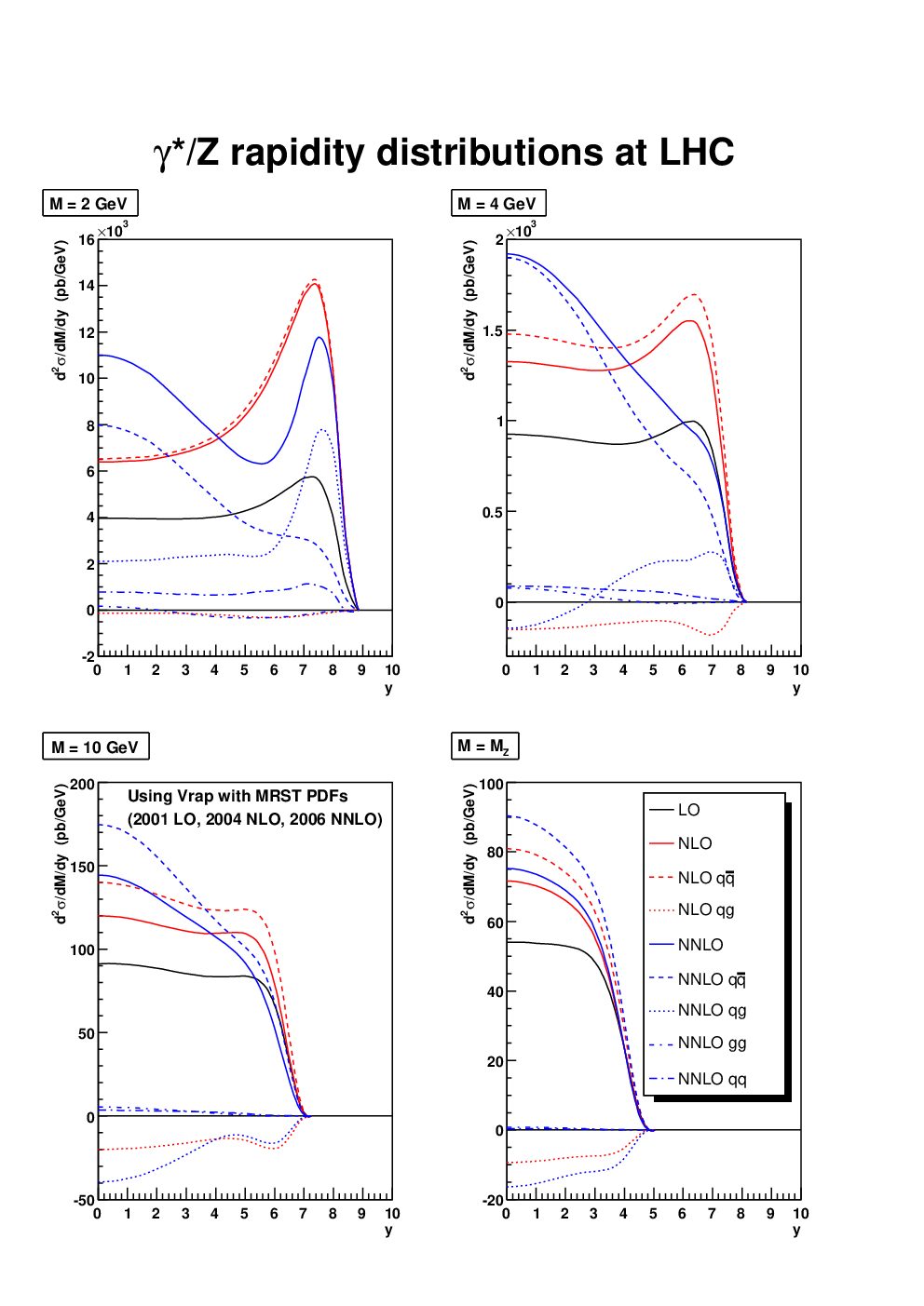
Hence, there is some question about the stability of cross-sections as one progresses to higher orders in the perturbative series. This may sometimes be related to the issue of resummations at large or small and whether these are important. In Section 2.7 we gave a preliminary discussion of the convergence at small . In Fig. 47 we see a comparison of the gluon distribution extracted from the global fit at LO, NLO and NNLO[26]. The additional positive small- contributions in the splitting function at each order lead to a smaller very small- gluon at each successive order. Hence, in this regime there is clearly fairly poor stability. This is similar for , though there is some compensation due to the NNLO coefficient function. A more dramatic consequence for this lack of convergence can be seen for the LHC. In Fig. 48[213] we show the LO, NLO and NNLO predictions for for and production at the LHC for centre-of-mass energy, as a function of rapidity and invariant mass. There is good stability in the predictions for very high final state masses, but it becomes worse at lower scales where is larger and large terms appear in the perturbative expansion, which are equivalent to . This suggests resummation may be necessary in this regime.
We note that at large there is enough information available to perform reliable approximations to fits at NNNLO, see e.g [214, 215], in the nonsinglet sector . This seems to lead to no significant difference to the results at NNLO, with a stabilisation in the values of , implying good theoretical convergence in the the kinematic region where these fits are performed.
4.2 Electroweak corrections
In principle the smallness of the electromagnetic and weak couplings should mean the corrections from this source are small. However, at high scales so they may be comparable to NNLO QCD corrections. Additionally there can be some enhancements, or violations of symmetry not present in QCD which can be important. The simplest thing one can consider is the QED–improved DGLAP equations which are,
| (87) |
at leading order in and , where
| (88) |
is the photon distribution and momentum is conserved:
| (89) |
f

There has been one detailed study of the effects of the QED evolution on the PDFs obtained via a global fit in [216]. Because there are not any enhancements in Eq. (87) the effect on the quark distributions of the QED corrections is negligible at small where the gluon contribution dominates the evolution. The main effect is that the gluon loses a little momentum to the photon in order for the momentum sum rule to be satisfied. At large , photon radiation from quarks leads to faster evolution, roughly equivalent to a slight shift in , i.e. . Overall, the QED effects are much smaller than many sources of uncertainty. However, the up quarks at high radiate more photons than down quarks due to the higher charge weighting. This leads to an automatic violation in the charge symmetry assumed in Eq. (45), as seen in Fig. 49, and this reduces the NuTeV anomaly in the measurement of [81, 82]. The other place where QED corrected PDFs are important is where an initial state photon plays a role. Consider the electroweak corrections to lepton pair production[217]. In the hard cross-sections the QED effects are typically a few percent and negative, becoming larger in magnitude at high transverse momentum. However, one also needs to consider photon-induced processes driven by the photon distribution of the proton, as shown in Fig. 50. Can be a significant fraction of the other electroweak corrections, and in the opposite direction, i.e. positive.

Large Electroweak corrections are potentially possible due to enhanced logarithms of the form in the perturbative series[218]. Jet cross-sections are an example[219] where there is potentially a big effect at LHC energies where is a very large number, as seen in Fig. 51. Similar results exist for corrections to other processes with a hard scale, e.g. di-boson production[220] and large- vector bosons in conjunction with jets[221] (though very sensitive to jet vetoes). These could potentially affect the extraction of PDFs at the LHC if they are not taken account of properly. In order to do this though, one must not only have virtual corrections for , but must have contributions of the form where the bosons are emitted as extra final state particles, which will certainly cancel the loop virtual corrections to some significant extent[222]. Whether the consideration of parton distributions with weak bosons as well as the photon will aid maximum precision since it is known that the evolution will produce electroweak double logarithms[223].

4.3 Small- Theory
As seen in Section 4.1 there are fairly strong hints of some instability, or lack of convergence in perturbation theory, when small- PDFs are probed. The reason for this instability was outlined in Section 2.7 – as known since[121, 122, 123] at each order in each splitting function and coefficient function generally obtains an extra power of . For the parton distributions these leading logarithms can be obtained from the BFKL equation for the high-energy limit of the unintegrated (in transverse momentum ) distribution
| (90) |
where is the unintegrated gluon distribution , and is a calculated kernel now known to NLO[224, 225]. The physical structure functions are then obtained from
| (91) |
is a calculable impact factor, known for structure functions[191, 226] and some other processes, e.g. [227]. As mentioned, the global fits usually assume that this is not significant in the region of interest, though a purely phenomenological investigation[228] did find that resummed terms were preferred by data.
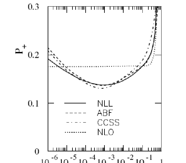
The inclusion of the NLO corrections to the BFKL equation and the consequent scale breaking made the solution much more difficult to obtain due to the difficulty of avoiding nonperturbative contamination from the infrared region. This led to a concentration of effort more closely related to the collinear factorisation of the usual perturbative ordering, and in particular the assumption that input PDFs should be fit and splitting functions and coefficient functions calculated. On this basis there has been good progress in incorporating resummation from essentially three groups [229, 230, 231] with results roughly in agreement, despite some differences in technique. In order to achieve stable results additional effects such as running coupling[232] effects and (depending on group) other corrections such as resummation of dominant collinear logarithms[233] are included. A comparison of the leading (mainly gluon) splitting function compared to the standard NLO result is shown in Fig. 52. It is a common result that the small- resummation leads to a dip for before the expected rise at very low in splitting functions and coefficient functions (though a full set of coefficient functions is still to come in some cases). A recent review of this work can be found in [152]. There are also approaches which attempt to predict the full structure functions, rather than just coefficient functions and splitting functions, e.g. [234, 235], though this must necessarily introduce some assumption about or modelling of the infrared physics. Results are encouraging, but it is more difficult to directly relate the PDFs and structure functions obtained to the standard fixed order ones using this type of approach.

A fit to data at NLO plus NLO resummation (in DIS scheme to NLO and a DIS-type resummed scheme beyond) with full resummation for heavy quarks included[229] has been performed. It leads to significant improvement in the fit to HERA data within a global fit and a change in the extracted gluon (Fig. 53), making it steeper at low and consequently slightly larger than the fixed-order gluon below at higher . Together with indications from Drell Yan resummation calculations[236] this suggests at least a few percent effect due to small- resummation at the LHC is quite possible, even for and bosons at higher rapidity. The resummed fit also produced a prediction for the HERA data on at low [126, 127, 128]. The results are seen in Fig. 54. The prediction is clearly successful, and gives additional evidence that resummation may be important, though there are other possible ways of explaining the excess over the NLO and NNLO perturbative predictions at small , which also means low , which leads us to the next topic.

4.4 Low , Higher Twist, Saturation
As noted in Section 1.2, the factorisation into coefficient functions and parton distributions is formally broken by corrections of . This effect is expected to be enhanced at high values of , and is related to the resummation of the perturbative corrections[237, 238, 239] which is formally divergent, leading to an ambiguity in the perturbation series which can be interpreted as power corrections or infrared renormalons[53, 54]. There have been numerous studies of higher twist contributions at high , e.g. [240, 143, 228, 241, 242, 215], and there is general agreement in the results. All studies find that the higher twist effects for and appear to be as expected from renormalon calculations, seen in Fig. 55, i.e. most important for high . They diminish with the perturbative order, i.e. at lower order they are mimicking the missing higher order effects, and appear to be stabilising in size by NNLO. Indeed, in those which have approximations to NNNLO[240, 241, 215] there is little difference, within uncertainties, to the higher twist extracted at NNLO. Hence, the series presumably reaches maximal convergence near NNNLO at high . For higher twist is a slightly larger effect at moderate , and this certainly seems to be the case in [143, 243], as predicted by the renormalon calculation[244] which is has no protection from any sum rule at small , as the Adler sum rule provides for nonsinglet . This nonsinglet higher twist correction for (which is unrelated to the gluon distribution) is another possible explanation (at least in part) of the apparent low- results in [126, 127, 128].

At low there has long been an expectation that higher twist effects related to the gluon should be important, mainly due to the fact that the gluon distribution is expected to be very large and hence recombination[245] and ultimately saturation effects should set in. Empirical investigations have suggested[228] that this is not the case, with higher twist effects again diminishing with order, but not being very significant beyond the LO estimate. Additionally, a study of absorptive corrections[246] does not imply a very big effect. It has been suggested that this is due to an accidental cancellation of large terms in , e.g. [247], and that large gluon induced higher twist will persist in other structure functions. However, it may also be related to the fact that the small- low- gluon extracted from full NLO and NNLO fits is actually not nearly as large as once expected, or often assumed in attempts to calculate higher twist, which are often built upon LO perturbative expansions where the gluon is much larger.
The subject of the gluon at small-, and the degree of saturation has become a very large topic of study, inspired by the discovery that within the dipole model for DIS scattering a simple model incorporating saturation could give a good fit to both inclusive and diffractive structure function data[248]. This has branched out into the colour glass condensate[249] approach to the small- gluon and is far too extensive a topic to summarise here. A brief discussion and summary of recent results and fits using the dipole model, saturation effects and the colour glass condensate can be found in [250], and a more recent review of the colour glass condensate in particular can be found in [251]. Here we simply note a couple of points. More recent and sophisticated treatments, including certainly heavy quarks (sometimes missed in early studies) and impact parameter-dependence, seem to find saturation being associated with rather lower and . The saturation scale scale for various treatments is illustrated in Fig. 56 is seen to be at very low even for , falling to even lower as rises (the average for inclusive processes is ). For truly quantitative results it is also necessary to match the calculations in these approaches to the PDFs obtained at higher and from the reliable results using the collinear factorisation theory, which is by no means trivial and certainly not automatic[253].

5 PDFs for LO Monte Carlo generators

A recent development in the study of PDFs has been the introduction of a different definition of parton distributions generally known as modified LO PDFs. These have arisen due to the frequent need to use generators for events at particle colliders which perform the cross section calculation only at LO in QCD. LO cross sections combined with LO PDFs is often a very inaccurate approximation, usually being rather too small in normalisation and sometimes also with the wrong shape. This can easily be understood if one considers that NLO matrix elements (and beyond) often give large positive corrections: at small due to divergent terms in the matrix elements; near threshold due to large corrections from soft-gluon emissions near the edge of phase space; and there can be numerically large corrections from analytic continuation from the space-like to time-like region, e.g. a factor in Drell-Yan production. Cross sections for hadro-production of , , Higgs bosons, , -production and jet production (including jets) all have NLO enhancements from at least one of these sources. -channel processes do not have these type of large corrections, and for e.g. single top or Higgs via vector boson fusion the NLO matrix-element correction is small. Such processes probe partons usually in the range of , i.e. neither very large or small.


The use of NLO PDFS in LO Monte Carlo generators has been suggested to counter this, since NLO PDFs are larger in some regions than at LO. Sometimes it does lead to better results, but sometimes even worse, particularly at small where NLO PDFs, especially the gluon distribution, can be much smaller than at NLO because they have been extracted with large positive contributions to quark evolution included at NLO. An alternative argument is that rather than the normal fixed order definitions this situation requires the introduction of new type of modified LO (LO*) PDF[254]. These allow the LO PDFs to be generally bigger by allowing momentum violation in global fits performed at LO, and can also use the NLO definition of , which is larger at low scales where much of the DIS data is fit than a LO with the same value at . As a further development one can also make the evolution more “Monte Carlo like”, by changing the renormalisation scale in the coupling from to something more like resulting in the LO** distributions[255]. In both cases the PDFs are obtained entirely from a fit to existing data, the quality of the LO* fit being much better than the rather poor LO result, but not quite as good as NLO. It was hoped that in the modified PDFs the enhancement in the partons compared to standard LO should compensate to some extent the missing NLO enhancements in the matrix elements. In[254] there was an extensive investigation of whether this idea works in practice. Comparison was made between predictions for a wide variety of processes made using the MC@NLO generator[256], which combines NLO matrix elements with parton showering, using NLO PDFs, and predictions using LO generators and LO, NLO and LO* PDFs. Taking the MC@NLO results to be the most accurate representation it was found that for the vast majority of cases the LO* gave the best results for the LO generators, particularly for gluon initiated processes, while sometimes standard LO and sometimes NLO gave the worst results. As an example we see in Fig. 57 the final state distributions for single and pairs[254], where the results using the LO* PDFs are almost identical to NLO.
The LO* MRST PDFs have been followed by parton distributions for event generators from the CTEQ collaboration[257]. The reasoning for the need for these PDFs is the same as for the LO* sets. However, the manner of obtaining them follows some of the same principles, but also has some different ones. Various sets have been produced, CT09MCS, CT09MC1 and CT09MC2. Some (CT09MC1 and CT09MC2) do allow the violation of the momentum sum rule and in CT09MC2 the NLO definition of the coupling is used. A major difference is that the PDFs are obtained by fits also including LHC “pseudodata” generated using full NLO calculations. This is different in philosophy to the LO* sets. It is noted that there is significant tension between the best fits to pseudodata and to the existing, largely structure function data. There is no modification of the scale of the coupling to make it more Monte Carlo like, but scales are varied to obtain the best quality fit to the pseudodata. An example of the comparison of the modified PDFs to standard LO and NLO PDFs is shown for the up quark in the right of Fig. 58. Clearly when momentum is violated the CT09MC quark is much larger than the fixed order over most values. This is unlike the MRST LO*/LO** quark in the left of Fig. 58, which is constrained at to give a good fit to high- HERA data. Inclusion of existing Tevatron data on rapidity, which postdates the LO* set would add some tension and should raise the quark distribution in this region a small amount. The gluon distributions in the two approaches are more similar, both being much bigger than fixed order at small . This is not surprising since the lack of direct constraint on the gluon distribution renders the differences in the approaches less important.


The comparison of the two types of PDF for gluon initiated processes is very similar. There is more difference in quark driven processes, such as and production. An example is shown in Fig. 59 which shows the rapidity distribution. The left-hand figure is from [257], and shows excellent agreement using CT09MC2, which is not surprising since the PDF as been obtained by fitting data of this type very well. The MRST LO* looks less successful in this plot. However, these results are from inclusive calculation with no parton showering as applied in generators. This can have a few percent effect, as seen in Section 3 of [257], and automatically includes some higher orders in the LO calculation. The right-hand plot from [255] does include parton showering in both LO and NLO calculations. The LO* results are somewhat nearer to NLO in this case since the LO calculation is a little nearer to NLO in this framework. Applying parton showering to the left hand plot must, on this evidence, improve the LO* comparison, and will affect the CT09MC2 comparison to some extent as well. There is no comparison to -channel processes in [257]. In [254] the enhancement of the PDFs led to these being marginally worse than LO PDFs. Even further enhancement is unlikely to be helpful.
An entirely different alternative is to obtain PDFs from fits using Monte Carlo generators directly. In detail this will then produce a slightly different PDF set for each generator, the details of parton showering differing between each. Work on this approach has been ongoing. However, it is rather more time intensive than normal fits, though there have been helpful developments[258], and results are so far limited. As noted near the beginning of Section 2 of this article, a very wide variety of data needs to be fit to provide true constraints on any PDFs, so it is not clear if this approach will lead to useful results in the immediate future.
6 Outlook
This review demonstrates the vast amount of progress that has taken place in the last years on pinning down the PDFs of the proton, as well as the dramatic increase in awareness of the impact of PDFs on the physics program of LHC experiments. LHC will need the best PDFs, especially for precision measurements, setting of limits in searches, and even for discoveries. Ideally the ATLAS and CMS (and LHCb and ALICE) analyses should follow a common procedure for using PDFs and their uncertainties in their key analyses. Also, changing frequently the PDFs in the software of the experiments, e.g. for cross–checks or the determination of error bands, is often non-trivial (e.g. due to the inter-connection with parameter choices for underlying event modelling, showering parameters and so on) and sometimes impractical if CPU intensive detector simulations are involved. LHC studies therefore will need both good central values for the PDFs to start with, and a good estimate of the associated uncertainties.
This has triggered the so called PDF4LHC initiative. PDF4LHC offers a discussion forum for PDF studies and information exchange between all stake-holders in the field. More details and links to the meetings so far can be found on the PDF4LHC web site [259]. Apart from getting the best PDFs, including the PDF uncertainties, based on the present data, another important deliverable is to devise strategies to use future LHC data to improve the PDFs. All this needs a close collaboration between theorists and those that are preparing to make the measurements. Such measurements include and production and asymmetries, di-jet production, hard prompt photons, Drell-Yan production, bottom and top quark production, Z-shape fits and Z+jets measurements. One expects that some of these channels can already be studied with first data at the LHC.
The final HERA data of run II (2004-2007) are still being analysed and will be very instrumental for future PDF fits, particularly for the high region. These data will become available in the next few years. Meanwhile interest is growing worldwide for a novel electron-ion collider. Design concepts exist at CERN, with ideas to intersect an electron accelerator with the Large Hadron Collider (LHeC)[260], and in the U.S. to either add an electron accelerator to the Relativistic Heavy Ion Collider at BNL, or an ion accelerator to the upgraded 12-GeV Continuous Electron Beam Accelerator Facility at JLab. The US project is generically called the EIC[261].

The LHeC has two alternative scenarios: a ring-ring (RR) scenario and a linac-ring (LR) scenario. For the RR scenario one typically has a 50 GeV electron beam on a 7 TeV proton beam (or 2.75 TeV heavy ion beam), and a peak luminosity of around cm-2s-1 for 50 MW power. The LR scenario has the potential to reach larger electron energies, perhaps up to 150 GeV, but in general the total integrated luminosity will by a factor 5 to 10 lower compared to the RR option.
The EIC projects discussed by BNL and JLab describe an electron beam of 4 to 20 GeV on a proton beam of 50 to 250 GeV. The peak luminosity aimed for is similar to the RR LHeC option. Polarization is an integral part of the proposal, aiming for 70% of polarization for each beam.
The kinematic reach covered by the LHeC is shown in Fig. 60 and for the EIC in Fig. 61. The high energy of the LHeC will allow to explore a new kinematic area for collisions, with values and values down to a few times . The high luminosity anticipated for the EIC and the possibility for polarized beams will allow for number a precision and novel measurements. It will however take us into the next decade before any future DIS data with much higher precision or larger kinematic domain will be available.
Further possible future constraints may come from the JLab experiments for the high- range with the new high intensity 12 GeV electron beam upgrade. The MINERvA experiment will use neutrino beams on nuclear targets at FNAL and is set to make precise measurements of neutrino cross sections with neutrino beams of energies up to roughly 30 GeV. MINERvA will collect 6M events on a carbon target in the transition (not so deep DIS) and DIS region plus an additional 6.5 M events in four nuclear targets and will significantly increase the existing neutrino data set available to the community. E906 is a new experiment at FNAL and is set to measure Drell-Yan production via muons. E906 will measure the ratio of the to distributions in the proton and the modifications to the quark sea in a nucleus. The expected statistics that will be collected is a factor 50 larger than that of E866/NuSea. The incoming proton beam energy will be only 120 GeV, reducing in the energy squared by a factor of 7 with respect to E866/NuSea. Thus the measurements of E906 will cover a different kinematic range, namely up to high values of 0.5. The run of E906 is scheduled to start in 2010 and to last for 2 years.
All these new data. together with ongoing theory developments will ensure that further improvements on the understanding and precision of the protons structure will continue in the next 1-2 decades.

7 Conclusions
Structure function measurements are a measure of the partonic structure of the proton and are instrumental in parton distribution function fits. The PDFs allow us to predict cross sections at particle colliders and a good knowledge of PDFs and their uncertainties is of prime importance for the success of the physics program of e.g. proton-proton collisions at the newly commissioned collider LHC.
Several versions of fits to data relevant for the hadron structure exist and all show that overall good quality fits using NLO or NNLO QCD can be obtained. Apart from the central values of the PDFs, it is essential to have also a good understanding of the uncertainties. Various ways of looking at uncertainties have been discussed in this paper, as used by the different fitting groups. The uncertainties are naively rather small – for a large number of PDFs and the predicted LHC quantities. Measurements of ratios, e.g. ratios can give extremely tight constraint on partons distributions. However, there are many effects in the fitting procedure that can contribute to the uncertainties, e.g. effects from input assumptions, in particular the selection of data fitted, cuts applied to the data and input parameterisation choices can shift the central values of predictions significantly and affect the size of uncertainties. During the last years it has also become clear that a complete heavy flavour treatment is essential in the extraction and use of the PDFs. Furthermore PDFs and are correlated and the uncertainties must be considered in tandem. These are all part of the Fixed Order QCD analysis, but there are additional effects. Electroweak corrections are often neglected but can potentially be large at very high energies following . Equally care must be taken for errors from higher orders/resummation, and power corrections/higher twist, which can be potentially large in certain phase space regions. Direct measurement of at HERA now give us some scope to test these predictions.
Since there is a spread in the PDFs obtained by the “global” fits which is indeed actually somewhat larger than the quoted uncertainties of each some procedure is required to estimate the “true” uncertainty associated with PDFs. If one is comparing to a measured cross-section then, of course, the comparison can and should be made to the prediction using any PDF set. In fact it is ideal to check as widely as possible to help determine which PDFs are most accurate in their predictions. However, if one is trying to determine the best value and uncertainty on a prediction in order to help set limits, determine the significance of a signal, or estimate uncertainty from extrapolation into certain regions of phase space, there is the need for some recommendation for a best prediction and a conservative, but representative uncertainty. This was requested, for example, for making benchmark predictions for Higgs boson cross-sections[262], and has been a major focus of the efforts of the afore-mentioned PDF4LHC group. If very high or very small PDFs are probed the lack of significant data constraints in some PDFs can lead to big variations – the minimum variation seems to be for , since all fits include HERA data, but also sum rules impose crossing points. However, the spread of the predictions[169, 263, 170] can be significant, even when the PDFs probed are in this range, as seen in Fig 45. Hence, it is the interim PDF4LHC recommendation[259, 264] that at NLO a conservative uncertainty should be the envelope of the predictions using NNPDF2.0, CTEQ6.6 and MSTW08 PDFs and their uncertainty, including that due to variations in . The centre of the envelope can be taken as the best prediction. An example of predictions using this is seen in Table 1. Since of these three sets MSTW is the one available at NNLO at present the central value should be taken from this, but the fractional uncertainty should be the same as at NLO in order to be conservative, also seen in Table 1. NNLO sets are available from ABKM, JR and most recently HERA, as described earlier in this article, and so ideally checks should also be made against these, though some deviations can be large. As seen the NNLO corrections themselves can be large for some processes. This recommendation is to be viewed as temporary and updates are expected. Another aim of the PDF4LHC group is to investigate, and hopefully minimise the spread between different sets, or at least to understand it as fully as possible. This will be aided by additional data as well as theoretical improvements, and will also inform future recommendations.
| nb | nb | nb | pb | pb | pb | pb |
| 7 TeV centre of mass energy (NLO) | ||||||
| 7 TeV centre of mass energy (NNLO) | ||||||
Hence, as well as testing for Beyond the Standard Model Physics the LHC can add significantly to our knowledge of the proton structure especially at low through measurement at high rapidities of hard probes, e.g. and Drell-Yan events. Indeed, the former is largely a precursor for the latter. The extraction of PDFs from existing data and use for LHC is still a far from straightforward procedure. We currently have the bare minimum of constraints required for constraining all PDFs over the full range required, and the a full understanding of PDF uncertainties related to experimental errors is still being developed. In addition there are many theoretical issues to consider to obtain real precision in some cases. At the LHC there will be relatively few cases where Standard Model discrepancies will not require some significant, and decidedly nontrivial input from PDF physics to determine their true significance.
Acknowledgements
RST would like to thank Alan Martin, Dick Roberts, James Stirling and Graeme Watt for many discussions on this subject during collaboration. Both authors would like to thank the members of the PDF4LHC steering committee for fruitful interaction over the past few years, as well as numerous other colleagues. RST would like to thank the IPPP, Durham for the award of a Research Associateship to aid travel funding.
References
- [1] M. Breidenbach, et al., Phys. Rev. Lett. 23 (1969) 935
- [2] E. Eichten, I. Hinchliffe, K. D. Lane, C. Quigg, Rev. Mod. Phys. 56 (1984) 579
- [3] J. G. Morfin, W. Tung Z. Phys. C 52 (1991) 13
- [4] A. D. Martin, R.G. Roberts, W.J. Stirling, Phys. Lett. B206 (1988) 327
- [5] J. D. Bjorken, Phys. Rev. 179 (1969) 1547
- [6] R. P. Feynman, Photon hadron Interactions, W.A. Benjamin, New York (1972)
- [7] G. Miller et al., Phys. Rev. D 5 (1972) 528
- [8] C. G. . Callan and D. J. Gross, Phys. Rev. Lett. 22 (1969) 156
- [9] R. K. Ellis, W. Furmanski and R. Petronzio, Nucl. Phys. B 212 (1983) 29
- [10] G. Altarelli and G. Parisi, Nucl. Phys. B 126 (1977) 298
- [11] L. N. Lipatov, Sov. J. Nucl. Phys. 20 (1975) 94 [Yad. Fiz. 20 (1974) 181]
- [12] V. N. Gribov and L. N. Lipatov, Sov. J. Nucl. Phys. 15 (1972) 438 [Yad. Fiz. 15 (1972) 781]
- [13] Y. L. Dokshitzer, Sov. Phys. JETP 46 (1977) 641 [Zh. Eksp. Teor. Fiz. 73 (1977) 1216]
- [14] D. J. Gross and F. Wilczek, Phys. Rev. D 8 (1973) 3633
- [15] H. Georgi and H. D. Politzer, Phys. Rev. D 9 (1974) 416
- [16] W. A. Bardeen, A. J. Buras, D. W. Duke and T. Muta, Phys. Rev. D 18 (1978) 3998
- [17] E. G. Floratos, D. A. Ross and C. T. Sachrajda, Nucl. Phys. B 129 (1977) 66 [Erratum-ibid. B 139 (1978) 545]
- [18] E. G. Floratos, D. A. Ross and C. T. Sachrajda, Nucl. Phys. B 152 (1979) 493
- [19] A. Gonzalez-Arroyo, C. Lopez and F. J. Yndurain, Nucl. Phys. B 153 (1979) 161
- [20] G. Curci, W. Furmanski and R. Petronzio, Nucl. Phys. B 175 (1980) 27
- [21] A. Gonzalez-Arroyo and C. Lopez, Nucl. Phys. B 166 (1980) 429
- [22] W. Furmanski and R. Petronzio, Phys. Lett. B 97 (1980) 437
- [23] E. G. Floratos, C. Kounnas and R. Lacaze, Nucl. Phys. B 192 (1981) 417
- [24] J. C. Collins, D. E. Soper and G. Sterman, Adv. Ser. Direct. High Energy Phys. 5 (1988) 1 [arXiv:hep-ph/0409313]
- [25] G. Altarelli, R. K. Ellis and G. Martinelli, Nucl. Phys. B 143 (1978) 521 [Erratum-ibid. B 146 (1978) 544]
- [26] A. D. Martin, W. J. Stirling, R. S. Thorne and G. Watt, Eur. Phys. J. C 63 (2009) 189 [arXiv:0901.0002 [hep-ph]]
- [27] P. M. Nadolsky et al., Phys. Rev. D 78, (2008) 013004 [arXiv:0802.0007 [hep-ph]]
- [28] R. D. Ball, L. Del Debbio, S. Forte, A. Guffanti, J. I. Latorre, J. Rojo and M. Ubiali, Nucl. Phys. B 838 (2010) 136 [arXiv:1002.4407 [hep-ph]]
- [29] F. D. Aaron et al. [H1 Collaboration and ZEUS Collaboration], JHEP 1001 (2010) 109 [arXiv:0911.0884]
- [30] S. Alekhin, J. Blumlein, S. Klein and S. Moch, Phys. Rev. D 81 (2010) 014032 [arXiv:0908.2766 [hep-ph]]
- [31] M. Gluck, P. Jimenez-Delgado and E. Reya, Eur. Phys. J. C 53 (2008) 355 [arXiv:0709.0614 [hep-ph]]
- [32] W. L. van Neerven and E. B. Zijlstra, Phys. Lett. B 272 (1991) 127
- [33] E. B. Zijlstra and W. L. van Neerven, Phys. Lett. B 273 (1991) 476
- [34] E. B. Zijlstra and W. L. van Neerven, Phys. Lett. B 297 (1992) 377
- [35] E. B. Zijlstra and W. L. van Neerven, Nucl. Phys. B 383 (1992) 525
- [36] S. Moch, J. A. M. Vermaseren and A. Vogt, Phys. Lett. B 606 (2005) 123 [arXiv:hep-ph/0411112]
- [37] J. A. M. Vermaseren, A. Vogt and S. Moch, Nucl. Phys. B 724 (2005) 3 [arXiv:hep-ph/0504242]
- [38] S. Moch, J. A. M. Vermaseren and A. Vogt, Nucl. Phys. B 688 (2004) 101 [arXiv:hep-ph/0403192]
- [39] A. Vogt, S. Moch and J. A. M. Vermaseren, Nucl. Phys. B 691 (2004) 129 [arXiv:hep-ph/0404111]
- [40] S. J. Brodsky, P. Hoyer, C. Peterson and N. Sakai, Phys. Lett. B 93 (1980) 451
- [41] S. Catani, D. de Florian, G. Rodrigo and W. Vogelsang, Phys. Rev. Lett. 93 (2004) 152003 [arXiv:hep-ph/0404240]
- [42] A. D. Martin, R. G. Roberts, W. J. Stirling and R. S. Thorne, Eur. Phys. J. C 4 (1998) 463 [arXiv:hep-ph/9803445]
- [43] L. W. Whitlow, E. M. Riordan, S. Dasu, S. Rock and A. Bodek, Phys. Lett. B 282 (1992) 475
- [44] A. C. Benvenuti et al. [BCDMS Collaboration], Phys. Lett. B 223 (1989) 485
- [45] M. Arneodo et al. [New Muon Collaboration], Nucl. Phys. B 483 (1997) 3 [arXiv:hep-ph/9610231]
- [46] M. R. Adams et al. [E665 Collaboration], Phys. Rev. D 54 (1996) 3006
- [47] L. W. Whitlow, Ph.D. thesis, Stanford University, 1990, SLAC-0357
- [48] A. C. Benvenuti et al. [BCDMS Collaboration], Phys. Lett. B 237 (1990) 592
- [49] M. Arneodo et al. [New Muon Collaboration], Nucl. Phys. B 487 (1997) 3 [arXiv:hep-ex/9611022]
- [50] U. K. Yang et al. [CCFR/NuTeV Collaboration], Phys. Rev. Lett. 86 (2001) 2742 [arXiv:hep-ex/0009041]
- [51] M. Tzanov et al. [NuTeV Collaboration], Phys. Rev. D 74 (2006) 012008 [arXiv:hep-ex/0509010]
- [52] G. Onengut et al. [CHORUS Collaboration], Phys. Lett. B 632 (2006) 65
- [53] Y. L. Dokshitzer, G. Marchesini and B. R. Webber, Nucl. Phys. B 469 (1996) 93 [arXiv:hep-ph/9512336]
- [54] M. Dasgupta and B. R. Webber, Phys. Lett. B 382 (1996) 273 [arXiv:hep-ph/9604388]
- [55] D. de Florian and R. Sassot, Phys. Rev. D 69 (2004) 074028 [arXiv:hep-ph/0311227]
- [56] K. J. Eskola, H. Paukkunen and C. A. Salgado, JHEP 0904 (2009) 065 [arXiv:0902.4154 [hep-ph]]
- [57] M. Hirai, S. Kumano and T. H. Nagai, Phys. Rev. C 76 (2007) 065207 [arXiv:0709.3038 [hep-ph]]
- [58] C. Adloff et al. [H1 Collaboration], Eur. Phys. J. C 19 (2001) 269 [arXiv:hep-ex/0012052]
- [59] C. Adloff et al. [H1 Collaboration], Eur. Phys. J. C 30 (2003) 1 [arXiv:hep-ex/0304003]
- [60] S. Chekanov et al. [ZEUS Collaboration], Phys. Lett. B 539 (2002) 197 [Erratum-ibid. B 552 (2003) 308] [arXiv:hep-ex/0205091]
- [61] S. Chekanov et al. [ZEUS Collaboration], Eur. Phys. J. C 32 (2003) 1 [arXiv:hep-ex/0307043]
- [62] G. Moreno et al., Phys. Rev. D 43 (1991) 2815
- [63] P. L. McGaughey et al. [E772 Collaboration], Phys. Rev. D 50 (1994) 3038 [Erratum-ibid. D 60 (1999) 119903]
- [64] J. C. Webb, Ph.D. thesis, New Mexico State University, 2002, arXiv:hep-ex/0301031; Paul E. Reimer, private communication (for the radiative corrections)
- [65]
R. Hamberg, W. L. van Neerven and T. Matsuura,
Nucl. Phys. B 359 (1991) 343
[Erratum-ibid. B 644 (2002) 403];
original code from http://www.lorentz.leidenuniv.nl/neerven/ - [66]
C. Anastasiou, L. J. Dixon, K. Melnikov and F. Petriello,
Phys. Rev. D 69 (2004) 094008
[arXiv:hep-ph/0312266];
Vrap code from http://www.slac.stanford.edu/lance/Vrap/ - [67]
K. Melnikov and F. Petriello,
Phys. Rev. D 74 (2006) 114017
[arXiv:hep-ph/0609070];
Fewz code from http://www.phys.hawaii.edu/kirill/FEHiP.htm - [68] M. Grazzini, arXiv:0908.1336 [hep-ph]
- [69] S. Catani, G. Ferrera and M. Grazzini, JHEP 1005 (2010) 006 [arXiv:1002.3115]
- [70] M. Arneodo et al. [New Muon Collaboration], Phys. Rev. D 50 (1994) 1
- [71] A. Baldit et al. [NA51 Collaboration], Phys. Lett. B 332 (1994) 244
- [72] R. S. Towell et al. [FNAL E866/NuSea Collaboration], Phys. Rev. D 64 (2001) 052002 [arXiv:hep-ex/0103030]
- [73] V. M. Abazov et al. [D0 Collaboration], Phys. Rev. D 76 (2007) 012003 [arXiv:hep-ex/0702025]
- [74] T. A. Aaltonen et al. [CDF Collaboration], Phys. Lett. B 692 (2010) 232 [arXiv:0908.3914 [hep-ex]]
- [75] A. O. Bazarko et al. [CCFR Collaboration], Z. Phys. C 65 (1995) 189 [arXiv:hep-ex/9406007] [76]
- [76] M. Goncharov et al. [NuTeV Collaboration], Phys. Rev. D 64 (2001) 112006 [arXiv:hep-ex/0102049]
- [77] F. Olness et al., Eur. Phys. J. C 40 (2005) 145 [arXiv:hep-ph/0312323]
- [78]
D. A. Mason,
“Measurement of the strange–antistrange asymmetry at NLO in QCD from
NuTeV dimuon data,”
FERMILAB-THESIS-2006-01;
“Final strange asymmetry results from NuTeV,”
Proceedings of 14th International Workshop on Deep Inelastic Scattering (DIS 2006), Tsukuba, Japan, 20-24 Apr 2006;
D. A. Mason et al., Phys. Rev. Lett. 99 (2007) 192001 - [79] H. L. Lai, P. Nadolsky, J. Pumplin, D. Stump, W. K. Tung and C. P. Yuan, JHEP 0704 (2007) 089 [arXiv:hep-ph/0702268]
- [80] S. Alekhin, S. Kulagin and R. Petti, Phys. Lett. B 675 (2009) 433 [arXiv:0812.4448 [hep-ph]]
- [81] G. P. Zeller et al. [NuTeV Collaboration], Phys. Rev. Lett. 88 (2002) 091802 [Erratum-ibid. 90 (2003) 239902] [arXiv:hep-ex/0110059]
- [82] G. P. Zeller et al. [NuTeV Collaboration], Phys. Rev. D 65 (2002) 111103 [Erratum-ibid. D 67 (2003) 119902] [arXiv:hep-ex/0203004]
- [83] T. Aaltonen et al. [CDF Collaboration], Phys. Rev. Lett. 102 (2009) 181801 [arXiv:0901.2169 [hep-ex]]
- [84] D. Acosta et al. [CDF Collaboration], Phys. Rev. D 71 (2005) 051104 [arXiv:hep-ex/0501023]
- [85] V. M. Abazov et al. [D0 Collaboration], Phys. Rev. D 77 (2008) 011106 [arXiv:0709.4254 [hep-ex]]
- [86] V. M. Abazov et al. [D0 Collaboration], Phys. Rev. Lett. 101 (2008) 211801 [arXiv:0807.3367 [hep-ex]]
- [87] H. L. Lai, M. Guzzi, J. Huston, Z. Li, P. M. Nadolsky, J. Pumplin and C. P. Yuan, Phys. Rev. D 82 (2010) 074024 [arXiv:1007.2241 [hep-ph]]
- [88] R. D. Ball et al. [The NNPDF Collaboration], arXiv:1012.0836 [hep-ph]
- [89] H. L. Lai et al., Phys. Rev. D 55, 1280 (1997) [arXiv:hep-ph/9606399]
- [90] M. Bonesini et al. [WA70 Collaboration], Z. Phys. C 38 (1988) 371
- [91] L. Apanasevich et al. [Fermilab E706 Collaboration], Phys. Rev. Lett. 81 (1998) 2642 [arXiv:hep-ex/9711017]
- [92] E. Laenen, G. Sterman and W. Vogelsang, Phys. Rev. Lett. 84 (2000) 4296 [arXiv:hep-ph/0002078]
- [93] V. M. Abazov et al. [D0 Collaboration], Phys. Lett. B 639 (2006) 151 [Erratum-ibid. B 658 (2008) 285] [arXiv:hep-ex/0511054]
- [94] R. Ichou and D. d’Enterria, Phys. Rev. D 82 (2010) 014015 [arXiv:1005.4529 [hep-ph]]
- [95] B. Abbott et al. [D0 Collaboration], Phys. Rev. Lett. 86 (2001) 1707 [arXiv:hep-ex/0011036]
- [96] A. A. Affolder et al. [CDF Collaboration], Phys. Rev. D 64 (2001) 032001 [Erratum-ibid. D 65 (2002) 039903] [arXiv:hep-ph/0102074]
- [97] A. Abulencia et al. [CDF - Run II Collaboration], Phys. Rev. D 75 (2007) 092006 [Erratum-ibid. D 75 (2007) 119901] [arXiv:hep-ex/0701051]
- [98] V. M. Abazov et al. [D0 Collaboration], Phys. Rev. Lett. 101 (2008) 062001 [arXiv:0802.2400 [hep-ex]]
- [99] T. Aaltonen et al. [CDF Collaboration], Phys. Rev. D 78 (2008) 052006 [arXiv:0807.2204 [hep-ex]]
- [100]
T. Kluge, K. Rabbertz and M. Wobisch,
arXiv:hep-ph/0609285;
http://projects.hepforge.org/fastnlo/. - [101] Z. Nagy, Phys. Rev. D 68 (2003) 094002 [arXiv:hep-ph/0307268]
- [102] Z. Nagy, Phys. Rev. Lett. 88 (2002) 122003 [arXiv:hep-ph/0110315]
- [103] N. Kidonakis and J. F. Owens, Phys. Rev. D 63 (2001) 054019 [arXiv:hep-ph/0007268]
- [104] H. L. Lai et al. [CTEQ Collaboration], Eur. Phys. J. C 12 (2000) 375 [arXiv:hep-ph/9903282]
- [105] J. Pumplin, D. R. Stump, J. Huston, H. L. Lai, P. M. Nadolsky and W. K. Tung, JHEP 0207 (2002) 012 [arXiv:hep-ph/0201195]
- [106] A. D. Martin, R. G. Roberts, W. J. Stirling and R. S. Thorne, Eur. Phys. J. C 23 (2002) 73 [arXiv:hep-ph/0110215]
- [107] A. D. Martin, R. G. Roberts, W. J. Stirling and R. S. Thorne, Phys. Lett. B 604, 61 (2004) [arXiv:hep-ph/0410230]
- [108] J. Pumplin, J. Huston, H. L. Lai, P. M. Nadolsky, W. K. Tung and C. P. Yuan, Phys. Rev. D 80 (2009) 014019 [arXiv:0904.2424 [hep-ph]]
- [109] S. Chekanov et al. [ZEUS Collaboration], Phys. Lett. B 547 (2002) 164 [arXiv:hep-ex/0208037]
- [110] S. Chekanov et al. [ZEUS Collaboration], Nucl. Phys. B 765 (2007) 1 [arXiv:hep-ex/0608048]
- [111] C. Adloff et al. [H1 Collaboration], Eur. Phys. J. C 19 (2001) 289 [arXiv:hep-ex/0010054]
- [112] M. Wobisch, Ph.D. thesis, RWTH Aachen, 2000, DESY-THESIS-2000-049
- [113] A. Aktas et al. [H1 Collaboration], Phys. Lett. B 653 (2007) 134 [arXiv:0706.3722 [hep-ex]]
- [114] S. Chekanov et al. [ZEUS Collaboration], Eur. Phys. J. C 42 (2005) 1 [arXiv:hep-ph/0503274]
- [115] C. Adloff et al. [H1 Collaboration], Eur. Phys. J. C 21 (2001) 33 [arXiv:hep-ex/0012053]
- [116] J. Breitweg et al. [ZEUS Collaboration], Eur. Phys. J. C 7 (1999) 609 [arXiv:hep-ex/9809005]
- [117] S. Chekanov et al. [ZEUS Collaboration], Eur. Phys. J. C 21 (2001) 443 [arXiv:hep-ex/0105090]
- [118] S. Chekanov et al. [ZEUS Collaboration], Phys. Rev. D 70 (2004) 052001 [arXiv:hep-ex/0401003]
- [119] S. Chekanov et al. [ZEUS Collaboration], Eur. Phys. J. C 28 (2003) 175 [arXiv:hep-ex/0208040]
- [120] A. D. Martin, W. J. Stirling, R. S. Thorne and G. Watt, Eur. Phys. J. C 64 (2009) 653 [arXiv:0905.3531 [hep-ph]]
- [121] L. N. Lipatov, Sov. J. Nucl. Phys. 23 (1976) 338 [Yad. Fiz. 23 (1976) 642]
- [122] E. A. Kuraev, L. N. Lipatov and V. S. Fadin, Sov. Phys. JETP 45 (1977) 199 [Zh. Eksp. Teor. Fiz. 72 (1977) 377]
- [123] I. I. Balitsky and L. N. Lipatov, Sov. J. Nucl. Phys. 28 (1978) 822 [Yad. Fiz. 28 (1978) 1597]
- [124] F. D. Aaron et al. [H1 Collaboration], arXiv:0805.2809 [hep-ex]
- [125] S. Chekanov et al. [ZEUS Collaboration], Phys. Lett. B 682 (2009) 8 [arXiv:0904.1092 [hep-ex]]
- [126] N. Raicevic [H1 and ZEUS Collaborations], Nucl. Phys. Proc. Suppl. 198 (2010) 75
- [127] B. Reisert [H1 and ZEUS Collaborations], PoS E PS-HEP2009 (2009) 309
- [128] H1. Collaboration, arXiv:1012.4355 [hep-ex]
- [129] C. Adloff et al. [H1 Collaboration], Z. Phys. C 72 (1996) 593 [arXiv:hep-ex/9607012]
- [130] C. Adloff et al. [H1 Collaboration], Phys. Lett. B 528 (2002) 199 [arXiv:hep-ex/0108039]
- [131] A. Aktas et al. [H1 Collaboration], Eur. Phys. J. C 45 (2006) 23 [arXiv:hep-ex/0507081]
- [132] A. Aktas et al. [H1 Collaboration], Eur. Phys. J. C 40 (2005) 349 [arXiv:hep-ex/0411046]
- [133] J. Breitweg et al. [ZEUS Collaboration], Eur. Phys. J. C 12 (2000) 35 [arXiv:hep-ex/9908012]
- [134] S. Chekanov et al. [ZEUS Collaboration], Phys. Rev. D 69 (2004) 012004 [arXiv:hep-ex/0308068]
- [135] S. Chekanov et al. [ZEUS Collaboration], JHEP 0707 (2007) 074 [arXiv:0704.3562 [hep-ex]]
- [136] F. D. Aaron et al. [H1 Collaboration], Eur. Phys. J. C 65 (2010) 89 [arXiv:0907.2643 [hep-ex]]
- [137] S. Chekanov et al. [ZEUS Collaboration], Eur. Phys. J. C 65 (2010) 65 [arXiv:0904.3487 [hep-ex]]
- [138] A. D. Martin, W. J. Stirling, R. S. Thorne and G. Watt, Phys. Lett. B 652 (2007) 292 [arXiv:0706.0459 [hep-ph]]
- [139] R. S. Thorne, A. D. Martin, W. J. Stirling and G. Watt, PoS D IS2010, 052 (2010) [arXiv:1006.2753 [hep-ph]]
- [140] R. D. Ball et al., arXiv:1101.1300 [hep-ph]
- [141] S. Chekanov et al. [ZEUS Collaboration], Phys. Rev. D 67 (2003) 012007 [arXiv:hep-ex/0208023]
- [142] A. M. Cooper-Sarkar, PoS D IS2010 (2010) 023 [arXiv:1006.4471 [hep-ph]]
- [143] S. Alekhin, Phys. Rev. D 68 (2003) 014002 [arXiv:hep-ph/0211096]
- [144] S. Alekhin, JETP Lett. 82 (2005) 628 [Pisma Zh. Eksp. Teor. Fiz. 82 (2005) 710] [arXiv:hep-ph/0508248]
- [145] S. Alekhin, K. Melnikov and F. Petriello, Phys. Rev. D 74 (2006) 054033 [arXiv:hep-ph/0606237]
- [146] S. Alekhin, presented at PDF4LHC meeting, DESY, Hamburg, Nov. 2010, S. Alekhin, J. Blumlein and S. O. Moch, PoS D IS2010 (2010) 021 [arXiv:1007.3657 [hep-ph]]
- [147] M. Gluck, E. Reya and A. Vogt, Z. Phys. C 53 (1992) 127
- [148] P. Jimenez-Delgado and E. Reya, Phys. Rev. D 79 (2009) 074023 [arXiv:0810.4274 [hep-ph]]
- [149] A. D. Martin, R. G. Roberts, W. J. Stirling and R. S. Thorne, Phys. Lett. B 443 (1998) 301 [arXiv:hep-ph/9808371]
- [150] C. D. White and R. S. Thorne, Eur. Phys. J. C 45 (2006) 179 [arXiv:hep-ph/0507244]
- [151] J. Blumlein, S. Riemersma, M. Botje, C. Pascaud, F. Zomer, W. L. van Neerven and A. Vogt, arXiv:hep-ph/9609400
- [152] Z. J. Ajaltouni et al., arXiv:0903.3861 [hep-ph]
- [153] A. Vogt, Comput. Phys. Commun. 170 (2005) 65 [arXiv:hep-ph/0408244]
- [154] G. P. Salam and J. Rojo, Comput. Phys. Commun. 180 (2009) 120 [arXiv:0804.3755 [hep-ph]]
- [155] R. D. Ball et al. [NNPDF Collaboration], Nucl. Phys. B 809 (2009) 1 [Erratum-ibid. B 816 (2009) 293] [arXiv:0808.1231 [hep-ph]]
- [156] D. Stump et al., Phys. Rev. D 65 (2002) 014012 [arXiv:hep-ph/0101051]
- [157] J. Pumplin, D. R. Stump and W. K. Tung, Phys. Rev. D 65 (2002) 014011 [arXiv:hep-ph/0008191]
- [158] J. Pumplin et al., Phys. Rev. D 65 (2002) 014013 [arXiv:hep-ph/0101032]
- [159] A. D. Martin, R. G. Roberts, W. J. Stirling and R. S. Thorne, Eur. Phys. J. C 28 (2003) 455 [arXiv:hep-ph/0211080]
- [160] J. Pumplin, Phys. Rev. D 81 (2010) 074010 [arXiv:0909.0268 [hep-ph]]
- [161] J. Pumplin, arXiv:0909.5176
- [162] W. T. Giele and S. Keller, Phys. Rev. D 58 (1998) 094023 [arXiv:hep-ph/9803393]
- [163] W. T. Giele, S. A. Keller and D. A. Kosower, arXiv:hep-ph/0104052.
- [164] L. Del Debbio, S. Forte, J. I. Latorre, A. Piccione and J. Rojo [NNPDF Collaboration], JHEP 0703, 039 (2007) [arXiv:hep-ph/0701127]
- [165] R. D. Ball, L. Del Debbio, S. Forte, A. Guffanti, J. I. Latorre, J. Rojo and M. Ubiali [NNPDF Collaboration], JHEP 1005 (2010) 075 [arXiv:0912.2276 [hep-ph]]
- [166] R. D. Ball et al. [The NNPDF Collaboration], Nucl. Phys. B 823 (2009) 195 [arXiv:0906.1958 [hep-ph]]
- [167] M. Dittmar et al., arXiv:hep-ph/0511119
- [168] S. Forte at PDF4LHC meeting, DESY, Hamburg, Oct. 23 2009
- [169] G. Watt, talk at PDF4LHC benchmarking meeting, CERN, March 26th, 2010, http://indico.cern.ch/conferenceDisplay.py?confId=87871; updated versions will appear at http://projects.hepforge.org/mstwpdf/pdf4lhc/
- [170] S. Alekhin, J. Blumlein, P. Jimenez-Delgado, S. Moch and E. Reya, Phys. Lett. B 697 (2011) 127 [arXiv:1011.6259 [hep-ph]]
- [171] A. M. Cooper-Sarkar, arXiv:0707.1593 [hep-ph]
- [172] E. Laenen, S. Riemersma, J. Smith and W. L. van Neerven, Nucl. Phys. B 392, 162 (1993)
- [173] B. W. Harris and J. Smith, Nucl. Phys. B 452 (1995) 109 [arXiv:hep-ph/9503484]
- [174] I. Bierenbaum, J. Blumlein and S. Klein, Nucl. Phys. B 820 (2009) 417 [arXiv:0904.3563 [hep-ph]]
- [175] M. Buza, Y. Matiounine, J. Smith and W. L. van Neerven, Eur. Phys. J. C 1 (1998) 301 [arXiv:hep-ph/9612398]
- [176] M. A. G. Aivazis, J. C. Collins, F. I. Olness and W. K. Tung, Phys. Rev. D 50 (1994) 3102 [arXiv:hep-ph/9312319]
- [177] R. S. Thorne and R. G. Roberts, Phys. Rev. D 57 (1998) 6871 [arXiv:hep-ph/9709442]
- [178] A. Chuvakin, J. Smith and W. L. van Neerven, Phys. Rev. D 61 (2000) 096004 [arXiv:hep-ph/9910250]
- [179] M. Kramer, F. I. Olness and D. E. Soper, Phys. Rev. D 62 (2000) 096007 [arXiv:hep-ph/0003035]
- [180] W. K. Tung, S. Kretzer and C. Schmidt, J. Phys. G 28 (2002) 983 [arXiv:hep-ph/0110247]
- [181] R. S. Thorne, Phys. Rev. D 73 (2006) 054019 [arXiv:hep-ph/0601245]
- [182] S. Forte, E. Laenen, P. Nason and J. Rojo, Nucl. Phys. B 834 (2010) 116 [arXiv:1001.2312]
- [183] R. S. Thorne and W. K. Tung, arXiv:0809.0714 [hep-ph]
- [184] J. R. Andersen et al. [SM and NLO Multileg Working Group], arXiv:1003.1241
- [185] J. C. Collins, Phys. Rev. D 58 (1998) 094002 [arXiv:hep-ph/9806259]
- [186] P. M. Nadolsky and W. K. Tung, Phys. Rev. D 79 (2009) 113014 [arXiv:0903.2667 [hep-ph]]
- [187] W. K. Tung, H. L. Lai, A. Belyaev, J. Pumplin, D. Stump and C. P. Yuan, JHEP 0702 (2007) 053 [arXiv:hep-ph/0611254]
- [188] R. S. Thorne, PoS D IS2010 (2010) 053 [arXiv:1006.5925 [hep-ph]]
- [189] J. Pumplin, H. L. Lai and W. K. Tung, Phys. Rev. D 75 (2007) 054029 [arXiv:hep-ph/0701220]
- [190] J. J. Aubert et al. [European Muon Collaboration], Nucl. Phys. B 213 (1983) 31
- [191] S. Catani, M. Ciafaloni and F. Hautmann, Nucl. Phys. B 366 (1991) 135
- [192] E. Laenen and S. O. Moch, Phys. Rev. D 59 (1999) 034027 [arXiv:hep-ph/9809550]
- [193] A. D. Martin, W. J. Stirling and R. S. Thorne, Phys. Lett. B 636 (2006) 259 [arXiv:hep-ph/0603143]
- [194] A. D. Martin, W. J. Stirling, R. S. Thorne and G. Watt, Eur. Phys. J. C 70 (2010) 51 [arXiv:1007.2624 [hep-ph]]
- [195] S. Kretzer, H. L. Lai, F. I. Olness and W. K. Tung, Phys. Rev. D 69 (2004) 114005 [arXiv:hep-ph/0307022]
- [196] M. Gluck, P. Jimenez-Delgado, E. Reya and C. Schuck, Phys. Lett. B 664 (2008) 133 [arXiv:0801.3618 [hep-ph]]
- [197] P. Jimenez-Delgado and E. Reya, Phys. Rev. D 80 (2009) 114011 [arXiv:0909.1711 [hep-ph]]
- [198] A. Guffanti and J. Rojo, arXiv:1008.4671 [hep-ph]
- [199] H. L. Lai, J. Huston, Z. Li, P. Nadolsky, J. Pumplin, D. Stump and C. P. Yuan, arXiv:1004.4624
- [200] C. Amsler et al. [Particle Data Group], Phys. Lett. B 667 (2008) 1
- [201] F. Demartin, S. Forte, E. Mariani, J. Rojo and A. Vicini, Phys. Rev. D 82 (2010) 014002 [arXiv:1004.0962 [hep-ph]]
- [202] M. Ubiali, R. D. Ball, L. Del Debbio, S. Forte, A. Guffanti, J. I. Latorre and J. Rojo, arXiv:1005.0397
- [203] S. Catani, D. de Florian and M. Grazzini, JHEP 0105 (2001) 025 [arXiv:hep-ph/0102227]
- [204] R. V. Harlander and W. B. Kilgore, Phys. Rev. Lett. 88 (2002) 201801 [arXiv:hep-ph/0201206]
- [205] C. Anastasiou and K. Melnikov, Nucl. Phys. B 646 (2002) 220 [arXiv:hep-ph/0207004]
- [206] V. Ravindran, J. Smith and W. L. van Neerven, Nucl. Phys. B 665 (2003) 325 [arXiv:hep-ph/0302135]
- [207] C. Anastasiou, K. Melnikov and F. Petriello, Phys. Rev. Lett. 93 (2004) 262002 [arXiv:hep-ph/0409088]
- [208] C. Anastasiou, K. Melnikov and F. Petriello, Nucl. Phys. B 724 (2005) 197 [arXiv:hep-ph/0501130]
- [209] O. Brein, A. Djouadi and R. Harlander, Phys. Lett. B 579 (2004) 149 [arXiv:hep-ph/0307206]
- [210] V. M. Abazov et al. [D0 Collaboration], Phys. Lett. B 670 (2009) 292 [arXiv:0808.1306 [hep-ex]]
- [211] A. Abulencia et al. [CDF Collaboration], J. Phys. G 34 (2007) 2457 [arXiv:hep-ex/0508029]
- [212] DØ Collaboration: DØNote 4403-CONF, DØnote 4750, DØnote 4573
- [213] R. S. Thorne, A. D. Martin, W. J. Stirling and G. Watt, arXiv:0808.1847 [hep-ph]
- [214] J. Blumlein, H. Bottcher and A. Guffanti, Nucl. Phys. B 774 (2007) 182 [arXiv:hep-ph/0607200]
- [215] A. N. Khorramian, H. Khanpour and S. A. Tehrani, Phys. Rev. D 81 (2010) 014013 [arXiv:0909.2665 [hep-ph]]
- [216] A. D. Martin, R. G. Roberts, W. J. Stirling and R. S. Thorne, Eur. Phys. J. C 39 (2005) 155 [arXiv:hep-ph/0411040]
- [217] C. M. Carloni Calame, G. Montagna, O. Nicrosini and A. Vicini, JHEP 0710 (2007) 109 [arXiv:0710.1722 [hep-ph]]
- [218] M. Ciafaloni, P. Ciafaloni and D. Comelli, Phys. Rev. Lett. 84 (2000) 4810 [arXiv:hep-ph/0001142]
- [219] S. Moretti, M. R. Nolten and D. A. Ross, Nucl. Phys. B 759 (2006) 50 [arXiv:hep-ph/0606201]
- [220] E. Accomando, A. Denner and A. Kaiser, Nucl. Phys. B 706 (2005) 325 [arXiv:hep-ph/0409247]
- [221] J. H. Kuhn, A. Kulesza, S. Pozzorini and M. Schulze, Nucl. Phys. B 797 (2008) 27 [arXiv:0708.0476 [hep-ph]]
- [222] U. Baur, Phys. Rev. D 75 (2007) 013005 [arXiv:hep-ph/0611241]
- [223] P. Ciafaloni and D. Comelli, JHEP 0511 (2005) 022 [arXiv:hep-ph/0505047]
- [224] V. S. Fadin and L. N. Lipatov, Phys. Lett. B 429 (1998) 127 [arXiv:hep-ph/9802290]
- [225] M. Ciafaloni and G. Camici, Phys. Lett. B 430 (1998) 349 [arXiv:hep-ph/9803389]
- [226] S. Catani and F. Hautmann, Nucl. Phys. B 427 (1994) 475 [arXiv:hep-ph/9405388]
- [227] R. D. Ball and R. K. Ellis, JHEP 0105 (2001) 053 [arXiv:hep-ph/0101199]
- [228] A. D. Martin, R. G. Roberts, W. J. Stirling and R. S. Thorne, Eur. Phys. J. C 35 (2004) 325 [arXiv:hep-ph/0308087]
- [229] C. D. White and R. S. Thorne, Phys. Rev. D 75 (2007) 034005 [arXiv:hep-ph/0611204]
- [230] M. Ciafaloni, D. Colferai, G. P. Salam and A. M. Stasto, JHEP 0708, 046 (2007) [arXiv:0707.1453 [hep-ph]]
- [231] G. Altarelli, R. D. Ball and S. Forte, Nucl. Phys. B 799 (2008) 199 [arXiv:0802.0032 [hep-ph]]
- [232] R. S. Thorne, Phys. Rev. D 64 (2001) 074005 [arXiv:hep-ph/0103210]
- [233] G. P. Salam, JHEP 9807 (1998) 019 [arXiv:hep-ph/9806482]
- [234] K. Golec-Biernat and A. M. Stasto, Phys. Rev. D 80 (2009) 014006 [arXiv:0905.1321 [hep-ph]]
- [235] H. Kowalski, L. N. Lipatov, D. A. Ross and G. Watt, Eur. Phys. J. C 70 (2010) 983 [arXiv:1005.0355 [hep-ph]]
- [236] S. Marzani and R. D. Ball, Nucl. Phys. B 814 (2009) 246 [arXiv:0812.3602 [hep-ph]]
- [237] G. Sterman, Nucl. Phys. B 281 (1987) 310
- [238] D. Appell, G. Sterman and P. B. Mackenzie, Nucl. Phys. B 309 (1988) 259
- [239] S. Catani and L. Trentadue, Nucl. Phys. B 327 (1989) 323
- [240] A. L. Kataev, G. Parente and A. V. Sidorov, Nucl. Phys. B 573 (2000) 405 [arXiv:hep-ph/9905310]
- [241] J. Blumlein and H. Bottcher, Phys. Lett. B 662 (2008) 336 [arXiv:0802.0408 [hep-ph]]
- [242] A. Accardi, M. E. Christy, C. E. Keppel, P. Monaghan, W. Melnitchouk, J. G. Morfin and J. F. Owens, Phys. Rev. D 81 (2010) 034016 [arXiv:0911.2254]
- [243] A. D. Martin, W. J. Stirling and R. S. Thorne, Phys. Lett. B 635 (2006) 305 [arXiv:hep-ph/0601247]
- [244] E. Stein, M. Meyer-Hermann, L. Mankiewicz and A. Schafer, Phys. Lett. B 376 (1996) 177 [arXiv:hep-ph/9601356]
- [245] A. H. Mueller and J. w. Qiu, Nucl. Phys. B 268 (1986) 427
- [246] G. Watt, A. D. Martin and M. G. Ryskin, Phys. Lett. B 627 (2005) 97 [arXiv:hep-ph/0508093]
- [247] J. Bartels, K. Golec-Biernat and L. Motyka, Phys. Rev. D 81 (2010) 054017 [arXiv:0911.1935]
- [248] K. J. Golec-Biernat and M. Wusthoff, Phys. Rev. D 59 (1998) 014017 [arXiv:hep-ph/9807513]
- [249] E. Iancu, A. Leonidov and L. D. McLerran, Nucl. Phys. A 692 (2001) 583 [arXiv:hep-ph/0011241]
- [250] L. Motyka, K. Golec-Biernat and G. Watt, arXiv:0809.4191 [hep-ph]
- [251] F. Gelis, E. Iancu, J. Jalilian-Marian and R. Venugopalan, arXiv:1002.0333
- [252] G. Watt and H. Kowalski, Phys. Rev. D 78 (2008) 014016 [arXiv:0712.2670 [hep-ph]]
- [253] R. S. Thorne, Phys. Rev. D 71 (2005) 054024 [arXiv:hep-ph/0501124]
- [254] A. Sherstnev and R. S. Thorne, Eur. Phys. J. C 55 (2008) 553 [arXiv:0711.2473 [hep-ph]]
- [255] A. Sherstnev and R. S. Thorne, arXiv:0807.2132 [hep-ph]
- [256] S. Frixione and B. R. Webber, JHEP 0206 (2002) 029 [arXiv:hep-ph/0204244]
- [257] H. L. Lai, J. Huston, S. Mrenna, P. Nadolsky, D. Stump, W. K. Tung and C. P. Yuan, JHEP 1004 (2010) 035 [arXiv:0910.4183]
- [258] A. Bacchetta, H. Jung, A. Knutsson, K. Kutak and F. Samson-Himmelstjerna, Eur. Phys. J. C 70 (2010) 503 [arXiv:1001.4675 [hep-ph]]
- [259] The web page of the PDF4LHC forum can be found at http://www.hep.ucl.ac.uk/pdf4lhc/
- [260] P. Newman, Deep Inelastic Scattering at the TeV Energy Scale and the LHeC Project, Nucl. Phys. Proc. Suppl. 191 (2009) 307, [arXiv:0902.2292]
- [261] A Deshpande, Physics and challenges of the electron ion collider, AIP Conf.Proc.980 (2008) 343
- [262] LHC Higgs Cross Section Working Group et al., arXiv:1101.0593 [hep-ph]
- [263] S. Alekhin et al., “The PDF4LHC Working Group Interim Report,” arXiv:1101.0536 [hep-ph]
- [264] M. Botje et al., “The PDF4LHC Working Group Interim Recommendations,” arXiv:1101.0538 [hep-ph]
- [265] M. Aliev, H. Lacker, U. Langenfeld, S. Moch, P. Uwer and M. Wiedermann, Comput. Phys. Commun. 182 (2011) 1034 [arXiv:1007.1327 [hep-ph]]