Laser cooling of a trapped particle with increased Rabi frequencies
Abstract
This paper analyses the cooling of a single particle in a harmonic trap with red-detuned laser light with fewer approximations than previously done in the literature. We avoid the adiabatic elimination of the excited atomic state but are still interested in Lamb-Dicke parameters . Our results show that the Rabi frequency of the cooling laser can be chosen higher than previously assumed, thereby increasing the effective cooling rate but not affecting the final outcome of the cooling process. Since laser cooling is already a well established experimental technique, the main aim of this paper is to present a model which can be extended to more complex scenarios, like cavity-mediated laser cooling.
pacs
03.67.-a, 42.50.LcI Introduction
The idea of laser cooling for neutral atoms was first suggested by Hänsch and Schalow [1] and independently for trapped ions by Wineland and Dehmelt [2]. Since light carries momentum as well as energy, scattering light on matter can result in significant changes of the vibrational energy of massive particles. Over the last decades, laser cooling techniques have been designed which allow the cooling of atoms and ions to the the micro and nanokelvin temperatures needed for quantum coherence and degeneracy [5, 3, 4]. Examples of which are Sisyphus cooling [6] and evaporative cooling [7]. In this paper we focus our attention on laser sideband cooling of a particle in a harmonic potential [8] which can be used for example to transfer single ions to their motional ground state with a very high precision [9, 10].
The idea of laser sideband cooling of a single trapped particle is relatively straightforward. If the trapping potential of the particle is strong enough for its motion to become quantised and if the corresponding phonon frequency is much larger than the spontaneous decay rate of the excited electronic state, it becomes possible to resolve the motional sidebands with the cooling laser. As a consequence, the excitation of the excited electronic state of the trapped particle on the red sideband is most likely accompanied by the annihilation of a phonon. When followed by the spontaneous emission of a photon, the particle returns into its electronic ground state without regaining a phonon which implies cooling. The cooling cycle only stops when the particle reaches a state with almost no phonons. The final population of excited vibrational states is in general very small and only due to highly off-resonant excitations of the ground state of the atom-phonon system.
The theory of laser cooling has already been studied in great detail in the literature. For reviews on this topic see for example Refs. [11, 12, 13, 14]. The first theoretical discussion of laser cooling with red-detuned light based on a combination of simple classical and quantum ideas can be found in Ref. [8] by Wineland and Itano. Lindberg and Stenholm later introduced the tool for a full quantum treatment of laser cooling by deriving a master equation for spontaneously emitting atoms with atomic recoil included [15] (cf. also Refs. [16, 17, 19, 18, 20]). An alternative but consistent analysis of the laser cooling of trapped ions in a running and in a standing wave configuration has been presented by Cirac et al. in Ref. [21]. The main result of these papers is a cooling equation of the form
| (1) |
where denotes the mean phonon number. The can be interpreted as transition rates between states with different phonon numbers and relate to actual cooling and heating rates. Moreover, one can show that the stationary state phonon rate is given by [15, 11, 21, 14]
| (2) |
Experimental results confirm the general dependence of this stationary state phonon number on the emission rate of the excited electronic state of the trapped particle and on its phonon frequency [23].
The purpose of this paper is to analyse the cooling process of a single trapped particle in a harmonic potential with fewer approximations than previously done in the literature. For example, we avoid the adiabatic elimination of the excited atomic state, thereby obtaining an analysis of the cooling process which applies for a much wider range of Rabi frequencies of the cooling laser. As a result we find that does not have to be small compared to the spontaneous decay rate and the laser detuning . For example, in the weak confinement regime with , the Rabi frequency can be as large as and in the strong confinement regime with , the Rabi frequency can be as large as without noticeably increasing the stationary state phonon number . This is an interesting observation, since the effective cooling rate scales as which increases rapidly when increases.
Our calculations are more straightforward than previous calculations, since we replace the atomic raising operator and the phonon annihilation operator by two new operators and . These correspond to particles that are neither atoms nor phonons and commute with each other. Most importantly, they provide a representation of the Hamiltonian which no longer contains atomic displacement operators. Instead it depends on terms like which take non-linear effects in the atom-phonon interaction into account [22]. In the following we use this Hamiltonian to obtain a manageable set of cooling equations which are differential equations for the time derivatives of expectation values. As in Refs. [15, 11, 21, 19, 14], we are interested in the dynamics of the cooling process on the very slow time scale given by the cooling rate which scales as with . The only approximation involved in the following calculations of stationary state phonon numbers and effective cooling rates is to neglect higher order terms in the Lamb-Dicke parameter .
The main purpose of this paper is to establish and test a framework for the modelling of laser cooling which can be extended relatively easily to more complex cooling scenarios like cavity-mediated laser cooling [24] and the study of possible quantum optical heating mechanisms in sonoluminescence experiments [25]. Cavity-mediated laser cooling for example has many similarities with laser cooling but due to being more complex there is more flexibility in choosing different scenarios and experimental parameters [26].
There are six sections in this paper. Section II introduces the master equation of a single laser-driven trapped particle. Section III uses this master equation to derive a closed set of 23 cooling equations. These simplify to a set of five equations in the weak confinement regime and to a single equation in the strong confinement regime, respectively. In Section IV we show that the phonon coherences and the mean phonon number always reach their stationary state. Section V presents cooling rates and stationary state phonon numbers and compares analytical and numerical results. Finally, we summarise our findings in Section VI. Mathematical details are confined to Apps. A–D.
II Theoretical model
Let us start by introducing the theoretical model and the experimental setup. It consists of a single cooling laser which drives a strongly confined single particle. As long as the trapping potential is approximately harmonic, we can describe the motional states of the atom by a harmonic oscillator Hamiltonian. In this section, we consider the motion of the trapped particle as quantised and introduce the model which allows us to predict the time evolution of its mean phonon number . The purpose of the cooling laser is to minimise the number of phonons in the motion of the particle in the direction of the laser. Cooling other vibrational modes requires additional cooling lasers.
II.1 The Hamiltonian
The Hamiltonian of a single trapped particle inside the free radiation field and with external laser driving can be written as
| (3) |
The first two terms are the free energy of the electronic states and of the quantised vibrational modes of the trapped particle. The third term describes the energy of the surrounding free radiation field. The last terms take the dipole interaction of the electronic states with the present electromagnetic fields, i.e. the laser and the free radiation field, into account. We now have a closer look at every term in this equation.
Suppose the particle is effectively a two-level system with ground state and excited state and the energies , , and denote the energy of a single atomic excitation, of a single phonon excitation, and of a single excitation of the modes of the free radiation field, respectively. Then we have
| (4) |
where the operators and are the atomic lowering and raising operator and where and are the phonon annihilation operator and the annihilation operator of a photon with wavevector and polarisation , respectively. These operators obey the commutator relation
| (5) |
which is the usual commutator relation for bosonic annihilation operators. All other photon commutators are equal to zero.
The final term in Eq. (3) describes the dipole interaction of the electronic states and of the trapped particle with the free radiation field and the applied laser field. Within the usual dipole approximation 11 1 This means, we assume that the size of the atom is small compared to the relevant optical wavelength., it can be written as
| (6) |
Here is the electron charge, is the dipole moment of the particle, i.e. the position operator of its outer electron with respect to the atomic nuclei at position , while and denote the electric field amplitude of the free radiation field and of the laser field at time , respectively. The dipole moment equals
| (7) |
where is a 3-dimensional complex vector. The electric field operators are given by
| (8) |
with being the quantisation volume of the free radiation field and being a unit length polarisation vector orthogonal to . Moreover, , , and are the amplitude, the wave vector of length , and the frequency of the applied laser field, respectively.
II.2 The displacement operator
In the following, we assume that the incoming laser field has the same direction as the quantised motion of the trapped particle, since this maximises the effect of the cooling laser. Considering this motion as quantised with the phonon annihilation operator from above, hence implies
| (9) |
where the Lamb-Dicke parameter is a measure for the steepness of the effective trapping potential seen by the ion [11]. Notice that Eq. (9) applies as long as the trapping potential seen by the atom does not depend on its respective electronic state. This means, the following calculations apply to a trapped ion and to a trapped neutral atom with a magical wavelength [27].
Taking Eq. (9) into account, we find that the laser Hamiltonian is a function of the particle displacement operator [28]
| (10) |
which is a unitary operator with
| (11) |
Using the polar coordinates and , putting the -axis in the direction of the cooling laser, and writing the general wave vector of length as
we find that
| (16) | |||||
where and are the and the component of the vector . Writing the Hamiltonian in Eq. (6) as a function of displacement operators, it becomes
| (17) | |||||
This equation shows that the cooling laser establishes a coupling between the electronic states and of the trapped particle and its quantised motion. As we shall see below, the coupling to the free radiation field is the origin of spontaneous emission and recoil effects.
II.3 Interaction picture
Before continuing our derivation of the master equation, it is convenient to transform the Hamiltonian in Eq. (3) into an interaction picture. To do so, we choose
| (18) |
with as in Eq. (4). Neglecting relatively fast oscillating terms as part of the usual rotating wave approximation, the interaction Hamiltonian ,
| (19) |
becomes
| (20) | |||||
Here denotes the detuning between the laser and the relevant atomic transition and and ,
| (21) |
are the usual laser Rabi frequency and the atom-field coupling constant.
II.4 Spontaneous emission and recoil
The interaction Hamiltonian in Eq. (20) is now the starting point for the usual derivation of the master equations. Suppose the state of the laser-driven trapped particle is at given by the density matrix , while the free radiation field is in its vacuum state . Taking this into account, the density matrix of the particle at time can be written as [29]
| (22) |
where denotes the typical response time of the environment, i.e. the typical time it takes the environment to absorb a photon from the free radiation field, and where
| (23) | |||||
The first term in Eq. (22) describes the subensemble with no photon emission in . The second term in this equation is the unnormalised state of the subensemble with an emission in [29]. Taking the time derivation of on the coarse grained time scale into account, we obtain the usual master equation
| (24) |
in Lindblad form, where is a non-Hermitian conditional Hamiltonian with being the corresponding no-photon time evolution operator.
In order to calculate and , one usually exploits second order perturbation theory. Since the displacement operator is a unitary operator, i.e.
| (25) |
the derivation of the conditional Hamiltonian remains exactly the same as in the case, where the motion of the particle is not quantised. This means, we find that
| (26) | |||||
where the spontaneous decay rate of the excited electronic state is given by
| (27) |
However, the reset operator now contains recoil terms. Proceeding as described in App. A, we find that
| (28) | |||||
where denotes the -component of the normalised dipole vector . The above reset operator is different from the one often used in the literature [11, 21, 19]. The reason for this is that the authors of these references only consider the case where , as it applies to certain atomic level schemes and laser configurations. The above reset operator is more general. It is also consistent with the reset operator of a free particle whose motion is not quantised. In this case, the displacement operator becomes a number and the integration over results indeed in . This expression is independent of , as it should.
III Cooling equations
The master equations which we derived in the previous section can now be used to derive differential equations for expectation values, so-called rate or cooling equations. However, this is not a straightforward task due to the presence of the displacement operator in Eq. (26). To overcome this problem, we now introduce two new operators and which replace the particle and the phonon operators and , respectively. Both operators describe neither electronic excitations nor phonons but provide nevertheless a natural description of trapped particles.
III.1 Transformation of the Hamiltonian
To simplify the Hamiltonian in Eq. (17), we now introduce a new annihilation operator as
| (29) |
Using the commutator relation (5) and the unitarity of in Eq. (30), i.e. the fact that
| (30) |
one can show that obeys the commutator relation
| (31) |
The operator differs from by the fact that its application not only transforms into but also induces a kick which displaces the particle.
Eqs. (5), (11), and (31) can now be used to derive for example the commutator relations
| (32) |
These can then be used to show that
| (33) |
The operators and and functions of them do not commute in general. This means, although substituting Eq. (31) into the interaction Hamiltonian into Eq. (17), simplifies it a lot, we do not yet have a Hamiltonian which can be analysed easily.
III.2 Time evolution of expectation values
The time derivative of the expectation value of a time-independent operator equals
| (38) |
The master equation in Eq. (24) hence implies that
| (39) | |||||
with as in Eq. (37). This equation describes the time evolution of the expectation value within the interaction picture which we introduced previously in Section II.3.
In the following we are especially interested in the time evolution of the mean phonon number ,
| (40) |
Using Eqs. (31) and (34), we find that this expression is the same as
| (41) |
with , , and defined as
| (42) |
To predict the time evolution of , we need to evaluate the time evolution of these three expectation values. As we shall see below, we only obtain a closed set of cooling equations, if we consider in addition the expectation values
| (43) |
and the expectation values defined in App. B. Since all of these variables are expectation values of Hermitian operators, they are real and their time evolution is given by real differential equations.
Let us first have a look at the operator expectation values and to . Using the master equation in Eq. (39) to calculate the time derivatives of these five variables, we find that
| (44) |
The factor in this equation,
| (45) |
depends explicitly on the direction of the emitting dipole moment. It relates to the parameter used in previous papers [11, 21, 19, 14] via the equation
| (46) |
The time derivatives of the relevant and mixed operator expectation values can be found in App. C. Below we simplify these equations with the help of an adiabatic elimination of all relatively fast evolving variables.
III.3 Weak confinement regime
We now have a closer look at the case, where the trapped particle experiences a relatively weak trapping potential and where the Lamb-Dicke parameter is much smaller than one. More concretely we assume in the following that
| (47) |
In addition we assume that the Rabi frequency and the detuning are at most comparable to and definitely not much larger. However, notice that we do not demand that is much smaller than . A closer look at the cooling equations in App. C shows that this choice of parameters causes the operator expectation values and to to evolve on a much slower time scale than all other relevant expectation values. The reason for this is that these variables are all or mixed operator expectation values which decay with the spontaneous atomic decay rate .
Taking this into account and eliminating , , , and to adiabatically from the system dynamics, we obtain a closed set of five effective cooling equations which applies after a relatively short transition time and which can be written as
| (48) | |||||
A closer look at Eq. (44) shows that the time derivatives of the operator expectation values , and to depend only on , , and . The calculation of the matrix therefore only requires the calculation of , , and which can be found in App. C. Substituting Eqs. (103), (106), (108), and (112) into Eq. (44), we find that can be written as
The first order matrix elements in this equations are given by
| (55) |
with defined as in Eq. (104). The non-zero matrix elements of in second order in and in first order in are given by
| (56) |
Proceeding as above, one can show that is up to second order in to a very good approximation given by
| (57) |
Moreover, we find that the coefficients to in Eq. (48) equal
| (58) |
in first order in . We now have a closed set of five differential equations which can be used to analyse the time evolution of the operator expectation values analytically and numerically. Notice that the weak confinement regime which we introduced in Eq. (47) does not allow for the adiabatic elimination of the operator coherences to , since these evolve in general on the same time scale as the particle population .
III.4 Strong confinement regime
Let us now have a closer look at the parameter regime where the phonon frequency and the detuning exceed the spontaneous decay rate and the Rabi frequency by at least one order of magnitude,
| (59) |
In this so-called strong confinement regime, the time scale separation in the dynamics of the trapped particle is different than in the previous subsection. The adiabatic elimination performed in the previous section does not apply. However, at least at the end of the cooling process when is already very small, we can assume that the expectation values , , , , and to evolve much faster than the operator population . This means, we can simplify the system dynamics via an adiabatic elimination of all expectation values other than . Doing so (cf. App. D), we obtain the effective cooling equation
| (60) |
The frequencies and in this equation are given by
| (61) |
up to second order in . It is obvious that is the effective cooling rate for strongly confined particles.
IV Stability analysis

In the strong confinement regime, the cooling process is governed by a single differential equation (cf. Eq. (60)) with an always positive cooling rate and an always positive stationary state phonon number . This means, in the strong confinement regime, the trapped particle always reaches its stationary state. However, it is not clear whether the same applies in the weak confinement regime, where the cooling process is described by five linear differential equations (cf. Eq. (48)). In this section, we therefore have a closer look at the dynamics induced by these equations.
To do so, we introduce the shifted operator expectation values
| (62) | |||||
This definition means that the tilde and the non-tilde variables differ only by the stationary state solutions of the non-tilde expectation values. Substituting Eq. (62) into Eq. (48), we find that
| (63) |
The stationary state solution of these effective cooling equations is the trivial one with all variables equal to zero. However, notice that the corresponding stationary state is only reached, if all eigenvalues of have negative eigenvalues.
IV.1 Time evolution for
We first have a closer look at the time evolution of the operator expectation values for . One can easily check that the eigenvalues of the matrix in Eq. (III.3) are in this case simply given by
| (64) |
Taking this into account and solving Eq. (63) analytically, we find that
This behaviour is illustrated in Fig. 1(a) which shows numerical solutions of the effective cooling equations in Eq. (63) for the case where the particles are initially in a coherent state. The first two phase diagrams show and as functions of and , respectively. The fact that all points lie on a circle means that the state of the particles remains (at least approximately) coherent throughout the cooling process. Fig. 1(a) moreover shows that the particle population and therefore also the mean phonon number (cf. Eq. (41)) in zeroth order in remains constant in time. This is exactly as one would expect. There cannot be any cooling without a coupling between the electronic and the vibrational states of the trapped particle. Higher order corrections in have to be taken into account.
IV.2 First order corrections
Calculating the eigenvalues of in Eq. (III.3) up to first order in , we obtain again Eq. (64). All of them are either zero or imaginary. However, there are some small corrections to the eigenvectors in first order in . As a result, the shifted particle population remains no longer constant in time but oscillates on the time scale given by the phonon frequency . This is illustrated in Fig. 1(b) which shows a numerical solution of the effective cooling equations in Eq. (63) with all first order corrections in taken into account. However, since the eigenvalues of have no real parts, does not reach its stationary state value. No cooling occurs.
IV.3 Second order corrections
Calculating again the eigenvalues of the matrix in Eq. (III.3) but now taking also the terms in second order in into account, we find that
| (79) |
Since the matrix element is always negative, all five eigenvalues of have negative real parts. This means, all tilde variables are damped away and tend to zero on the time scale given by . This is illustrated in Fig. 1(c) which illustrates a numerical solution of Eq. (63).
Since the coherences to do not increase in time but oscillate instead with a slowly decreasing amplitude around constant values, the cooling process remains stable and the trapped particle eventually reaches its stationary state. This observation is taken into account in the following section, where we analyse the cooling process in more detail. It allows us to replace the coherences to by their time averages. This means, in the weak confinement regime, the calculations in the following section apply only towards the end of the cooling process, i.e. after a transition time of the order of.
V Cooling rates and phonon numbers
Taking the results of the previous section into account, replacing the operator coherences to by their time averages, and adiabatically eliminating all rapidly evolving expectation values, we obtain an effective cooling equation of the same form as the effective cooling equation in Eq. (60). The reason for this is that the time averages of the coherences to are exactly the same as the quasi-stationary state solutions obtained when setting their time derivatives in Eq. (48) equal to zero. The solution of Eq. (60) implies that the mean phonon number at time can to a very good approximation be written as
| (80) |
in zeroth order in with , since and are the same for . Notice that the general solution in Eq. (80) applies in the strong as well as in the weak confinement regime, although in the weak confinement regime only after a transition time of the order of . In this section, we derive analytical expressions for the stationary state phonon number and for the effective cooling rate in this equation which are much more general than the expressions which we obtained already in Section III.4. Afterwards, we show that these rates are in good agreement with numerical solutions of the closed set of 23 cooling equations which can be found in Section III.2 and App. C.
V.1 Stationary state phonon numbers
Using these cooling equations and setting the time derivatives of all expectation values equal to zero, we obtain the stationary state phonon number
| (81) |
with the frequencies , , and defined as
| (82) | |||||
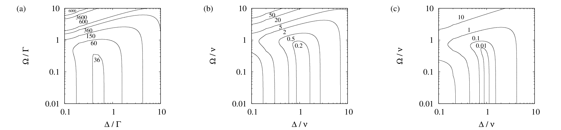
This result applies in zeroth order in without any approximations and is the main result of this paper. Fig. 2 shows as a function of the two laser parameters and for different experimental parameters. In the weak confinement regime one should choose . However, for and one should choose close to in order to minimise the final kinetic energy of the trapped particle.
Fig. 2 moreover shows that depends only weakly on the Rabi frequency which implies that effective laser cooling is not restricted to laser Rabi frequencies much smaller than as it is often implied in the literature [15, 21, 19, 14]. This is an interesting result, since larger ’s yield higher cooling rates , as we shall see below. Our numerical simulations show that can be as large as in the weak confinement and as large as in the strong confinement regime without noticeably increasing the final phonon number . However notice that for ’s larger than that, cooling changes quickly into heating, since increases relatively rapidly beyond certain critical points.
Let us now have a closer look at different parameter regimes to emphasize that our results are consistent with previous calculations. For example, for relatively small Rabi frequencies , Eq. (81) simplifies to
| (83) | |||||
This equation is in good agreement with the stationary state phonon number implied in Refs. [11, 21, 19, 14] for . This can be shown using Eqs. (2) and (46) in this paper and the expressions for in Eq. (7) in Ref. [19]. However, notice that the in this paper are slightly different from later definitions of the [14, 13].
V.1.1 Weak confinement

In the weak confinement regime, the stationary state phonon number in Eq. (83) simplifies to
| (84) |
Exactly the same stationary state phonon number is obtained when setting the left hand side of the five effective cooling equations in Eq. (44) equal to zero. This confirms the consistency of the calculations in this paper. As already pointed out above, for small , this expression assumes its minimum if
| (85) |
For this laser detuning and Rabi frequencies , the stationary state phonon number simplifies to
| (86) |
which is much larger than one.
V.1.2 Strong confinement
Using the effective cooling equation derived in Section III.4, we find that the stationary state phonon number in the strong confinement regimes equals
| (87) |
to a very good approximation. Exactly the same result is obtained when neglecting terms proportional to and in Eq. (81). This result suggests immediately that one should choose
| (88) |
in order to minimise the final phonon number . When substituting this detuning into Eq. (83), we find that the stationary state phonon number for laser sideband cooling is for relatively small Rabi frequencies to a very good approximation given by
| (89) |
which is much smaller than one [8].
V.2 Effective cooling rates
Proceeding as above but eliminating only the expectation values other than adiabatically from the time evolution of the trapped particle, we find that the effective cooling rate in Eq. (80) is in second order in given by
| (90) |
with and as in Eq. (82). Fig. 3 shows this cooling rate as a function of the laser parameters and . Indeed we find that increases in general as increases. This confirms that one should choose in general as large as possible without noticeably decreasing the stationary state phonon number .
For relatively small Rabi frequencies , i.e. for , the cooling rate in Eq. (90) simplifies to
| (91) |
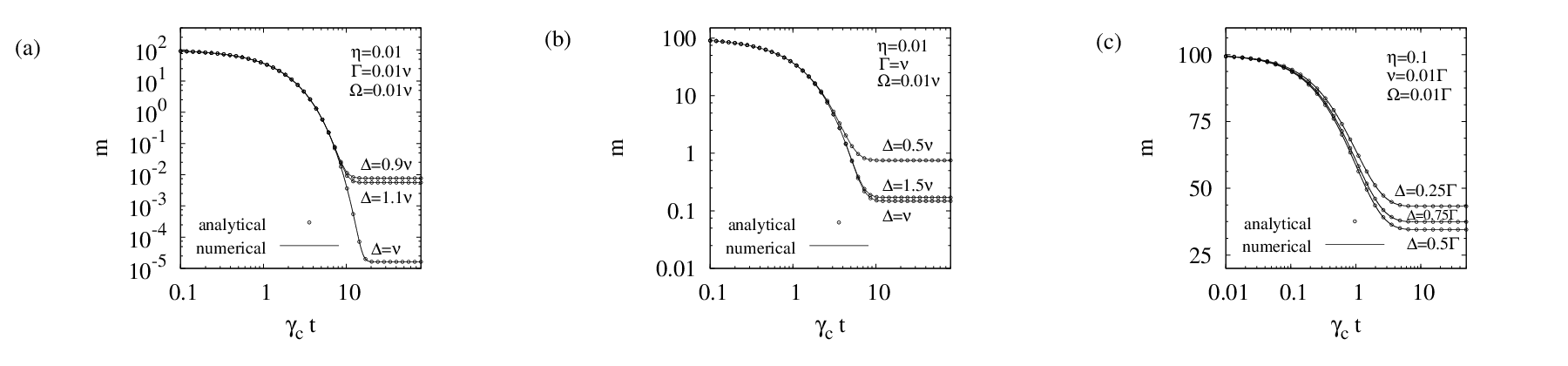
When comparing this result with the expression for in [11, 19], we find that our cooling rate is essentially the same as the cooling rate reported in these earlier references. Moreover, as Fig. 4 confirms, Eq. (90) is in very good agreement with numerical solutions.
V.2.1 Weak confinement
In the weak confinement regime, the laser detuning which minimises the stationary state phonon number is given by (cf. Eq. (85)). Taking this into account, the cooling rate in Eq. (90) simplifies to
| (92) |
in the limit of weak driving, ie. when neglecting terms proportional to . As Fig. 4(c) illustrates, this cooling rate is in good agreement with a numerical solution of the full set of 23 rate equations.
V.2.2 Strong confinement
In the strong confinement regime, terms which scale as or are in general negligible (cf. Eq. (59)). Taking this into account and simplifying Eq. (90) accordingly, we find that the cooling rate in this equation is exactly the same as in Eq. (61). The cooling process becomes indeed the most efficient, when the detuning is close to the phonon frequency (cf. Eq. (88)). The cooling rate is in this case given by
| (93) |
which is essentially the stationary state photon emission rate of a laser-driven atom multiplied by .
VI Conclusions
This paper analyses the cooling process of a single trapped particle with red-detuned laser light. In contrast to previous authors [11, 19, 21, 14, 13], our analysis avoids the adiabatic elimination of the excited atomic state when calculating the effective cooling rate and the stationary state phonon number . Our calculations hence apply to a wider range of laser Rabi frequencies . They show that can be chosen relatively large without affecting the final outcome of the cooling process. As illustrated in Fig. 2, in the weak confinement regime with , the Rabi frequency can be as large as and in the strong confinement regime with , the Rabi frequency can be as large as without reducing the stationary state phonon number noticeably. This is an interesting observation, since scales as and increases rapidly when increases.
The main novelty of our calculations is a transformation of the original Hamiltonian which replaces the atomic lowering operator and the phonon annihilation operator by two new operators and which commute with each other. The corresponding particles are neither atomic excitations nor phonons but provide a more natural description of the trapped particle. Our calculations are therefore more straightforward than previous calculations. Since the theory of laser cooling has already been studied in great detail in the literature [11, 12, 13, 14], the main purpose of this paper is to establish and test a framework for the modeling of laser cooling which can be extended relatively easily to more complex cooling scenarios like cavity-mediated laser cooling [24, 26] and possible quantum optical heating mechanisms in sonoluminescence experiments [25].
Acknowledgement. This work was supported by the UK Research Council EPSRC. N. S. S. acknowledges funding from The Ministry of Education in Saudi Arabia.
Appendix A Derivation of the reset state
Substituting the interaction Hamiltonian in Eq. (20) into the expression for in Eq. (23) and using first order perturbation theory we find that
| (94) | |||||
Using the concrete expression for in Eq. (20), the relation
| (95) |
and ignoring an overall level shift which can be absorbed into the free energy of the system, the reset operator becomes
| (96) | |||||
This expression can be evaluated relatively easily in the large volume limit, where
when using the same notation as in Section II.2. Performing the integration implied by this equation, using Eqs. (17) and (21), and writing the normalised dipole moment as
| (98) |
we finally find that is indeed given by Eq. (28). The spontaneous decay rate in this equation is the same as in Eq. (27). Notice that denotes the component of the normalised dipole moment in the direction of the cooling laser.
Appendix B Relevant expectation values
The calculations in the following two appendices require in addition to the expectation values defined in Section III.2 the operator expectation values
| (99) |
Moreover we employ the mixed operator expectation values
| (100) |
and
| (101) |
The time derivatives of these and other expectation values which we defined in Sec. III.2 can be found in App. C. Notice that this paper does not introduce expectation values and to . These names are reserved for variables which are used in other cooling scenarios.
Appendix C , , and in the weak confinement regime
Setting and substituting the operator expectation values , , and into Eq. (39), we find that they evolve according to
| (102) |
in zeroth order in . These equations form a closed set of differential equations. Eliminating all -operator expectation values adiabatically which change on the relatively fast time scale given by and adopting a notation where , with the superscript indicating the scaling of the respective term with respect to , we find for example that is in zeroth order in given by
| (103) |
The constant in this equation is given by
| (104) |
In addition to , we obtain solutions for and . These will be used in the next subsection to calculate the coherences and up to first order in .
Setting and using again Eq. (39), we find that the time evolution of the mixed operator coherences and and to is in zeroth order in given by
| (105) |
All six expectation values evolve on the relatively fast time scale given by the spontaneous decay rate . Taking this into account and eliminating them adiabatically in the weak coupling regime, i.e. for relatively small , we find that
| (106) |
to a very good approximation. The constant is given in Eq. (104) above. In addition to and we obtain expressions for and . These are used in the next subsection to calculate up to first order in .
Proceeding as above but taking terms up to first order in into account we find that the first order in contributions of the operator expectation values , , and in Eq. (43) evolve according to
| (107) |
These equations form a closed set of cooling equations, when the results for and which we obtained in App. C are taken into account. Eliminating , and adiabatically
| (108) |
in the weak confinement regime which we introduced in Section III.3. This means terms proportional to have been neglected.
In order to calculate and up to first order in , we need a closed set of cooling equations which holds correctly up to this order. Applying Eq. (39) again to and and to , we find that
| (109) | |||||
Substituting the definitions of the mixed-particle expectation values , and and to into Eq. (39) and setting , we find that
| (110) |
while
| (111) |
These final six differential equations hold in zeroth order in . Setting the right hand side of these and of the cooling equations in Eq. (109) equal to zero, we finally find that
| (112) |
in the weak confinement regime. This means, terms of order have again been neglected. Fig. 5 compares the above analytical results for , , and with the result of a numerical solution of the above cooling equations. Very good agreement between both solutions is found which suggests that the effective cooling equations in Eq. (48) apply after a very short transition time of the order .

Appendix D , and in the strong confinement regime
The calculation of in zeroth order in is the same as in App. C. However, in the strong confinement regime, the expression in Eq. (103) simplifies to
| (113) |
Setting and eliminating the operator coherences adiabatically from the system dynamics we immediately find that to all equal zero in zeroth order in ,
| (114) |
Taking this into account when eliminating the mixed operator expectation values whose time derivatives are given in Eq. (105), we moreover find that
| (115) |
To calculate the coherences and up to first order in , we have a look at the time derivatives of , , and to in first order in which can be found in Eq. (109). Combining Eqs. (111) and (114), we immediately see that
| (116) |
Taking this and the expressions for , , , and obtained in App. C into account, when setting the time derivatives of the relatively fast evolving variables in Eq. (109) equal to zero, we therefore find that
| (117) |
These coherences are different from the coherences in Eq. (112), since they apply only in the strong confinement regime. As Fig. 6 shows there is again very good agreement between the analytical and the numerical solutions for , , and . This means that the effective cooling equation for the strong confinement regime in Eq. (60) too applies after a relatively short transition time.

References
- [1] T. Hänsch and A. Schawlow, Opt. Comm. 13, 68 (1975).
- [2] D. Wineland and H. Dehmelt, Bull. Am. Phys. Soc. 20, 637 (1975).
- [3] S. Chu, Rev. Mod. Phys. 70, 685 (1998).
- [4] C. N. Cohen-Tannoudji, Rev. Mod. Phys. 70, 707 (1998).
- [5] W. D. Phillips, Rev. Mod. Phys. 70, 721 (1998).
- [6] C. Cohen-Tannoudji and W. Philips, Phys. Today 43, 33 (1990).
- [7] W. Ketterle and N. J. VanDruten, Adv. in Atom. and Mol. Phys. 37, 181 (1996).
- [8] D. J. Wineland and W. M. Itano, Phys. Rev. A 20, 1521 (1979).
- [9] F. Diedrich, J. C. Bergquist, W. M. Itano, and D. J. Wineland, Phys. Rev. Lett. 62, 403 (1989).
- [10] C. Monroe, D. M. Meekhof, B. E. King, S. R. Jefferts, W. M. Itano, D. J. Wineland, and P. Gould, Phys. Rev. Lett. 75, 4011 (1995).
- [11] S. Stenholm, Rev. Mod. Phys. 58, 699 (1986).
- [12] G. Z. K. Horvath, R. C. Thompson and P. L. Knight, Contemp. Phys. 38, 25 (1997).
- [13] D. Leibfried, R. Blatt, C. Monroe, and D. Wineland, Rev. Mod. Phys. 75, 281 (2003).
- [14] J. Eschner, G. Morigi, F. Schmidt-Kaler, and R. Blatt, J. Opt. Soc. Am. B 20, 1003 (2003).
- [15] M. Lindberg and S. Stenholm, J. Phys. B 17, 3375 (1984).
- [16] S. Stenholm, Appl. Phys. 15, 287 (1978).
- [17] M. Lindberg, J. Phys. B 17, 2129 (1984).
- [18] J. Javanainen, M. Lindberg, and S. Stenholm, J. Opt. Soc. Am. B 1, 111 (1984).
- [19] S. Stenholm, J. Opt. Soc. Am. B 2, 1743 (1985).
- [20] J. Dalibard and C. Cohen-Tannoudji, J. Phys. B 18, 1661 (1985).
- [21] J. I. Cirac, R. Blatt, P. Zoller, and W. D. Phillips, Phys. Rev. A 46, 2668 (1992).
- [22] W. Vogel and R. L. de Matos Filho, Phys. Rev. A 52, 4214 (1995).
- [23] C. Raab, J. Eschner, J. Bolle, H. Oberst, F. Schmidt-Kaler, and R. Blatt, Phys. Rev. Lett. 85, 538 (2000).
- [24] A. Beige, P. L. Knight, and G. Vitiello, New J. Phys. 7, 96 (2005).
- [25] A. Kurcz, A. Capolupo, and A. Beige, New J. Phys. 11, 053001 (2009).
- [26] T. Blake, A. Kurcz, and A. Beige, J. Mod. Opt. 58, 1317 (2011).
- [27] J. McKeever, J. R. Buck, A. D. Boozer, A. Kuzmich, H.-C. Nägerl, D. M. Stamper-Kurn, and H. J. Kimble , Phys. Rev. Lett. 90, 133602 (2003).
- [28] C. C. Gerry and P. L. Knight, Introductory Quantum Optics, Cambridge University Press (Cambridge, 2005).
- [29] G. C. Hegerfeldt, Phys. Rev. A 47, 449 (1993).