CMB Fluctuations and String Compactification Scales

Observation of cosmic microwave background (CMB) [1] provides a great opportunity for testing fundamental theories. It is generally believed that the fluctuations of CMB originate from quantum fluctuations generated at energy much higher than present accelerators can achieve.

It is hoped that string theory gives predictions for observational cosmology. But at the current stage of its development, string theory is defined only in limited classes of background spacetimes. The analysis of cosmology has been limited to those based on low energy effective field theory, and it has been difficult to make concrete predictions. (For attempts to formulate cosmology beyond the level of effective field theory, see e.g. [2] and [3].)

In this Letter we will focus on an aspect of fundamental theories, namely the presence of a large number of fields. These could be Kaluza-Klein (KK) modes from the compactification of extra dimensions or excited states of strings. Our analysis is mostly based on effective field theory, but we will also use a general property of perturbative string theory as an input.

It would be possible that the size of extra dimensions $L$ is large in unit of Hubble scale of inflation $H^{-1}$. We already know a hierarchy of scales between the Planck scale $m_{pl}$ and $H$: The fact that tensor perturbation (B-mode polarization of CMB) has not been observed implies $H$ is at least 4 orders of magnitude smaller than $m_{pl}$ [1]. The question is whether string scale $m_{s}$ is close to $m_{pl}$ or $H$. We will see below that with $m_{s}$ slightly smaller than $H\sim 10^{-4}m_{pl}$, $L$ can be as large as $L\sim 10^{8}H^{-1}$. In such a case, there will be many KK modes with $m\lesssim H$. We will show that the quantum effects of these fields lead to interesting observable effects.

For concreteness, we shall consider a collection of $N$ free fields $\phi_{A}$ ($A=1,\ldots,N$) with mass $m_{A}$, which are classically at the bottom of the potential $\phi_{A}=0$. We will not consider inflaton field, and take the background to be pure de Sitter, and find the temperature fluctuations generated during inflation. At the end of this Letter, we make comments on the effect of time dependence of Hubble, e.g. near the end of inflation.

In this Letter we point out that temperature fluctuations $\delta T/T$ can be generated by a mechanism different from the standard one based on slow-roll inflation. In the latter case, the classical value of a scalar field (inflaton) provides a preferred time slicing, and its fluctuation is interpreted as the difference of duration of inflation at different points in space, which results in the density (or temperature) anisotropy. In our case, the fields $\phi_{A}$ are classically at rest, and the above argument does not apply. It has been assumed that these fields do not contribute to $\delta T/T$. We will show that by keeping quadratic terms in $\phi_{A}$, the gravitational potential $\Phi$ is generated through quantum effects of these fields. Each field gives small contribution, but when $N\gg 1$, this effect becomes important. The large ratio between scalar and tensor contributions to $\delta T/T$ is usually assumed to be the consequence of the smallness of the slope of the inflaton potential. In our approach, it is the consequence of a large number of fields.

In the following, we first review quantization in de Sitter space, and recall that fields with $m<{3\over 2}H$ do not oscillate at super-horizon scales, because the “friction” due to the cosmic expansion overdumps the oscillation. These are the fields that we will focus on. We then study Einstein equations and solve for the gravitational potential $\Phi$ in terms of the matter fields. Using this, we find the contribution to CMB fluctuations from KK modes. We will make an argument based on string perturbation theory that if string scale $m_{s}$ is lower than $H$, the summation over the mass is effectively cut off at $m_{s}$. We then use the observed data on the amplitude of $\delta T/T$ and the tensor-to-scalar ratio $r_{t/s}$ to constrain the parameters, such as $m_{s}$ and $L$.

There have been inflationary models involving a large number of fields. In “N-flation” [4] (or “assisted inflation” [5]), many fields (such as axions) classically roll down the potential, collectively producing an effect similar to chaotic inflation. Our mechanism is different from this, since we are not assuming classical motion. Also note that our mechanism is different from the curvatons scenario [6]. We demonstrate that curvature fluctuations are generated during inflations without such a late time mechanism.

We consider background de Sitter space

and a collection of $N$ free massive scalar fields,

In the following we will often use the conformal time, $\tau=\int dt/a(t)=-e^{-Ht}$ ($-\infty\leq\tau\leq 0$), and the rescaled field $\chi_{A}=a\phi_{A}$ which has the standard kinetic term. We will suppress the label $A$ hereafter for brevity.

Fourier component of $\chi$ satisfies the equation of motion (prime denotes $\partial_{\tau}$),

Quantization is done by setting

where $u_{\vec{k}}(\tau)$ is the solution of (3) which approaches $u_{\vec{k}}(\tau)\to e^{-i|\vec{k}|\tau}$ at early time $\tau\to-\infty$. This condition ensures that the flat space result is recovered in the short distance limit. The solution is given by $u_{\vec{k}}(\tau)=\sqrt{\pi\over 2}e^{i{\pi\over 2}(\nu+{1\over 2})}\sqrt{-|\vec{k}|\tau}H_{\nu}^{(1)}(-|\vec{k}|\tau)$ with $\nu=\sqrt{{9\over 4}-m^{2}H^{-2}}$. Asymptotic behavior at the late times (in the super-horizon $|\vec{k}|/a\ll H$ limit) is $u_{\vec{k}}\sim(-|\vec{k}|\tau)^{-\nu+{1\over 2}}$. Time dependence factorizes from space dependence, as is clear from the fact that $|\vec{k}|$ dependence drops out from (3) in this limit. Fields with small mass, $mH^{-1}<{3\over 2}$, do not oscillate in time. We will take the $mH^{-1}\ll 1$ limit in the following formulas, since this is the case of importance for our applications, as explained below.

The equal time two-point function of $\phi$ at late times is

where we have taken the $m^{2}H^{-2}\ll 1$ limit, and defined

Quantum fluctuations of the fields $\phi$ induce gravitational potential. Let us look at the (0, $i$) and ($i$, $j$) components of the Einstein equation,

where $\mathcal{H}={a^{\prime}\over a}=-{1\over\tau}$. The l.h.s is the Einstein tensor expanded to the first order in metric fluctuations; $\Phi$ and $\Psi$ are the two gauge invariant combinations constructed from the scalar modes (See e.g. [8]). On the r.h.s. we have energy momentum tensor which is quadratic in $\phi$,

The sum is taken over the species of the fields. The superscript ${\rm(S)}$ denotes the scalar part (the part which can be written as derivatives of a scalar), e.g.,

We shall use the Einstein equation to express $\Phi$ and $\Psi$ in terms of the matter fields $\phi$. We first find the difference $\Phi-\Psi$ from the $(i\neq j)$ component of (8),

and substitute it into (7) to get

At late times, the r.h.s. goes like $(-\tau)^{\beta-1}$, which implies $\Phi\sim(-\tau)^{\beta}$. The part containing $s$ can be dropped when $\beta\ll 1$, since this gives smaller contribution in correlation functions than the second term¹¹ 1 In correlation functions, ${\partial\over\partial x^{i}}\langle\phi(x)\phi(x^{\prime})\rangle$ gives a factor of order $\beta$ (and further differentiation only gives order 1 factors like $-(\beta+1)$). Correlators involving the first term of (11) necessarily contain more of these factors than the ones involving only the second term of (11).. Using the fact that time dependence ($\phi\sim(-\tau)^{\beta/2}$) enters as a multiplicative factor, and $\partial_{i}(\phi\partial_{i}\phi)={1\over 2}{\bigtriangleup}\phi^{2}$, we find

at late times and $\beta\ll 1$. This satisfies all the components of Einstein equations. The connected part of two-point function becomes²² 2 The expectation value (one-point function) of $\Phi$ is UV divergent, but the two-point function is not. As long as we are studying the connected part of two-point functions, we do not need renormalization.

Next we consider tensor fluctuations. The transverse-traceless (TT) mode of gravitons ($\nabla^{i}h_{ij}$=$h^{i}_{i}$=0) is sourced by the TT part of energy-momentum tensor,

The general solution to this equation is the sum of the solution $h^{(0)}_{ij}$ for the homogeneous equation and a particular solution $h^{(1)}_{ij}$ which depends on $\delta T^{(T)}_{ij}$. This means that the tensor fluctuation consists of the usual gravitational wave $h^{(0)}_{ij}$ on top of the piece $h^{(1)}_{ij}$ which is determined by $\delta T^{(T)}_{ij}$. Since the homogeneous equation is equivalent to massless scalar equation, $h^{(0)}_{ij}$ scales logarithmically (in space and time), giving rise to the scale invariant spectrum with the amplitude $H/m_{pl}$. On the other hand, $h^{(1)}_{ij}$ decays in time ($h^{(1)}_{ij}\sim(-\tau)^{\beta+2}$, since $\delta T^{(T)}_{ij}\sim(-\tau)^{\beta}$), so the effect of $\delta T^{(T)}_{ij}$ is unimportant at late times.

Let us now assume that a part of the extra dimensions is compactified on a manifold with the size $L\gg H^{-1}$, and find temperature fluctuations produced by the KK modes. For simplicity, we assume $D$ dimensions are compactified on $T^{D}$ with the same periodicity $L$ in all directions, and the other dimensions are compactified on a space with the string scale size. KK modes from $T^{D}$ have mass $m^{2}=\sum_{a=1}^{D}(2\pi n_{a})^{2}/L^{2}$. Assuming the level is sufficiently dense, the number of states is given by $S_{D-1}|n|^{D-1}d|n|=S_{D-1}(L/2\pi)^{D}m^{D-1}dm$, where $S_{D-1}=2\pi^{D/2}/\Gamma(D/2)$ is the volume of the $D-1$ dimensional unit sphere.

In this Letter, we only consider scalar fields. There are also vector and tensor KK modes, but as long as we are considering quantum fluctuations around vanishing expectation values, they behave similarly to massive scalars, and just contribute extra multiplicities³³ 3 We do not have problems of anisotropy, since vectors and tensors have zero expectation values. Even if they aquire non-zero expectation values after inflation, the anisotropy will be suppressed as $1/\sqrt{N}$ when there are $N$ independent fields. See [7] for discussion in a closely related context..

The two point function of $\Phi$ (13) becomes

where $c_{D}=S_{D-1}/(4(2\pi)^{D+2})$. The upper limit $m_{c}$ of the integration should be $m_{c}\sim{3\over 2}H$ as long as we are working in Einstein gravity. However, if string scale is less than Hubble scale, $m_{s}<H$, string states should be taken into account. In this case, we expect that the sum over the mass is effectively cut off at $m_{c}\sim m_{s}$ for the following reason. Let us assume the two-point function of $\Phi$ comes from the one-loop diagram in string theory. String theory can be regarded as a field theory with infinitely many fields, except that one-loop amplitude effectively has UV cutoff due to modular invariance; Schwinger proper time is cut off at string scale. There is no physical meaning to time interval shorter than string scale, or oscillations much higher than string scale. This means the internal states in the loop which has mass much larger than string scale do not have physical effect⁴⁴ 4 This argument is based on string theory in flat background, and it is not clear whether this can be applied to an arbitrarily curved background, but we believe this is a reasonable estimate. In fact, the precise value of this cutoff does not affect our final conclusion: The preferred value of the string scale, being about one order lower than Hubble scale, is not modified even if we take the upper limit to be $(3/2)H$ instead of $m_{s}$..

Temperature fluctuation of CMB is related to $\Phi$ at recombination (at redshift $z\sim 1100$) by ${\delta T/T}=-\Phi/3$. The angle $\theta$ on the sky corresponds to the distance $d_{r}=2R_{r}\sin(\theta/2)$ where $R_{r}\sim H_{0}^{-1}$ is the radius of the surface of last scattering. We are interested in the modes outside the horizon at recombination, which correspond to $3^{o}\leq\theta$ ($l\leq 60$). For these modes, $\Phi$ will be frozen (remain constant at fixed comoving distance) after inflation. Thus we will look at the correlator at distance ${(a_{e}/a_{r})}d_{r}=2R\sin(\theta/2)=a_{e}|\vec{x}-\vec{x^{\prime}}|$ at the end of inflation, where $a_{e}$ and $a_{r}$ are the scale factors at the end of inflation and at recombination. The radius $R=(a_{e}/a_{r})R_{r}$ will depend on the scale of inflation. We will assume $RH\sim 10^{29}\sim e^{67}$ in the following.

The power spectrum $C_{l}$ is defined by $\langle{\delta T\over T}(\theta){\delta T\over T}(0)\rangle=\sum_{l=1}^{\infty}(2l+1)C_{l}P_{l}(\cos\theta)$. To find it, let us expand

and recall that $-2\log(\sin(\theta/2))$ is $1/(l(l+1))$ in harmonic space. The square amplitude $\delta^{2}_{T}\equiv l(l+1)C_{l}$ becomes

where we have taken the upper limit to be $m_{c}=m_{s}$. This is a good approximation even when $m_{s}>H$, since the contribution from the region $m\gtrsim H/10$ will be strongly suppressed due to the factor $(2RH)^{-{4\over 3}m^{2}H^{-2}}$ in any case. We have defined

To see the qualitative behavior of $\delta^{2}_{T}$, it would be helpful to note ${\cal M}_{D}(\zeta_{0})\sim\zeta_{0}^{-{D+2\over 2}}$ when $\zeta_{0}\gg 1$. In this limit, we have $\delta^{2}_{T}\sim({H\over m_{pl}})^{4}(LH)^{D}(\log(2RH))^{-{D+2\over 2}}$ up to constant factors. $\delta^{2}_{T}$ is enhanced when extra dimensions are large, $(LH)^{D}\gg 1$, since many fields contribute to it. $\delta^{2}_{T}$ becomes small if $\log(2RH)$ were larger, since massive fields weakly decay in time during inflation.

We will now use observational data [1],

to constrain the parameters in our model. This implies ${H\over m_{pl}}=\sqrt{\frac{9\pi}{2}\delta_{\text{T}}^{2}r_{\text{t/s}}}\lesssim 0.81\times 10^{-4}$. Let us first assume this inequality is saturated. Then the amplitude (16) provides the relation between the two parameters $m_{s}$ and $L$, or equivalently, between $m_{s}$ and the string coupling $g_{s}$, since $L$ is written as $(Lm_{s})^{D}=8\pi^{6}g_{s}^{2}(m_{pl}^{2}/m_{s}^{2})$.

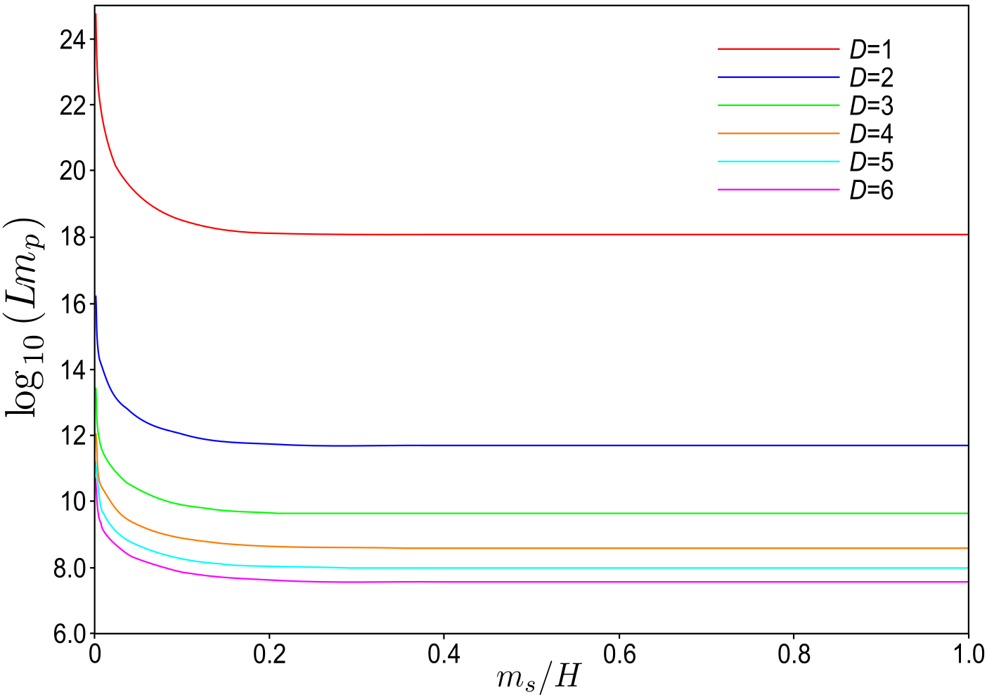
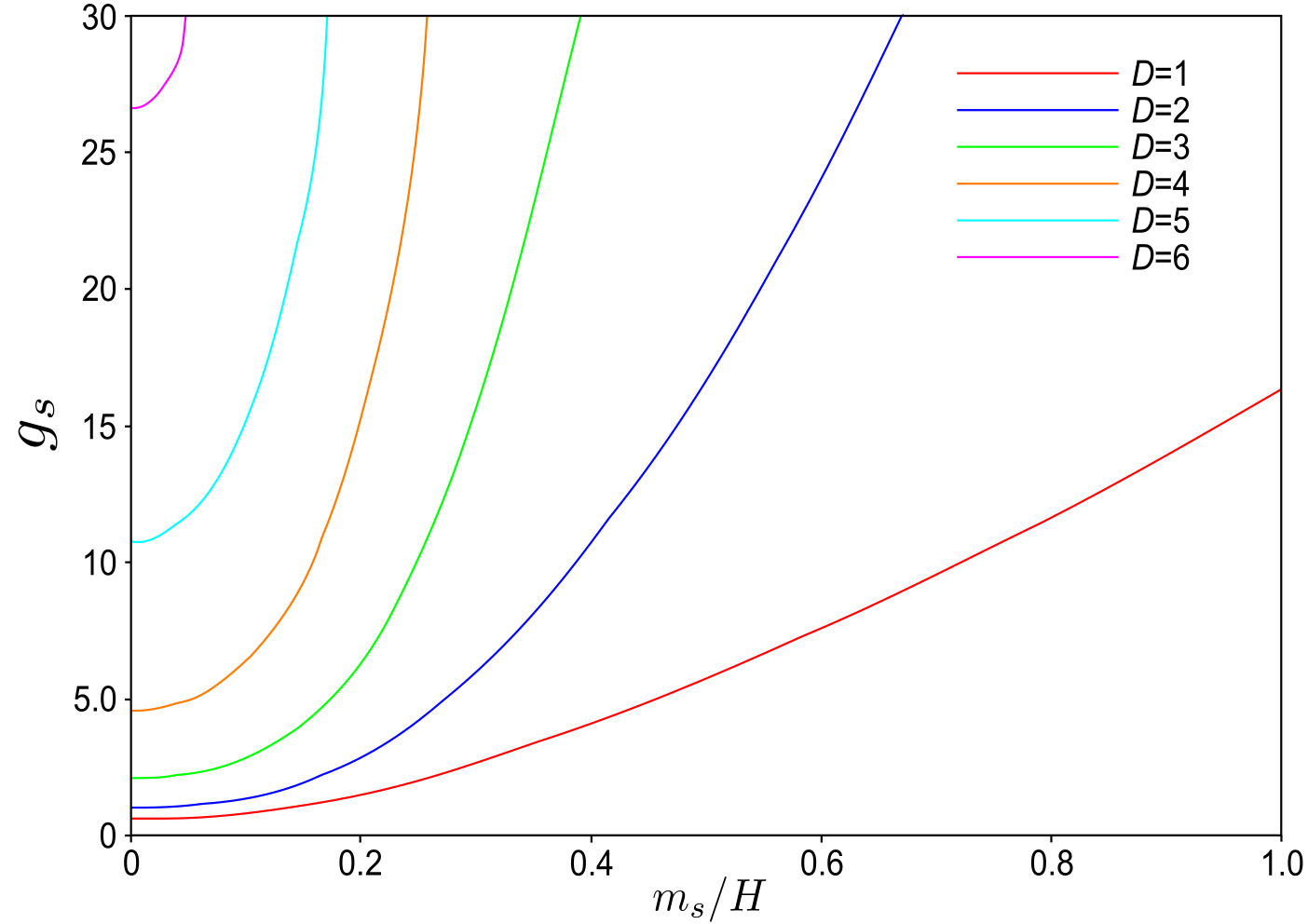
Figs. 1 and 2 show $(Lm_{pl})$ and $g_{s}$ as functions of $m_{s}/H$, respectively. It is easier to have weak coupling with small $D$, while it is easier to keep $L$ not too large with large $D$. Typical values that are consistent with (18) would be: $\{D=2,m_{s}/H=0.2,Lm_{pl}=10^{12},g_{s}=3\}$, $\{D=3,m_{s}/H=0.2,Lm_{pl}=10^{10},g_{s}=5\}$, $\{D=4,m_{s}/H=0.1,Lm_{pl}=10^{9},g_{s}=7\}$. The number of the fields that participate in $\delta T/T$ is roughly $N\sim(Lm_{s})^{D}$. For the above choice of parameters, $10^{14}\lesssim N\lesssim 10^{16}$. The fact that $m_{s}$ is close to $H$ (or slightly smaller) in our model can be understood as follows: If we include quantum expectation value of the scalar fields on the r.h.s. of Friedmann equation during inflation, we should have $H^{2}\gtrsim NH^{4}/m_{pl}^{2}$. Our values of $H$ and $N$ do not satisfy this. This implies corrections (characterized by $H/m_{s}$) are so large that Friedmann equation is not applicable.

Since $\delta T/T$ originates from the fluctuations of massive fields, the spectrum is slightly stronger in the UV, thus the spectral index $n_{s}$ is larger than 1 in our model,

This is in the range $1\lesssim n_{s}\lesssim 1.02$ when $D=2$, and $1\lesssim n_{s}\lesssim 1.05$ for $D\leq 6$.

The three-point function of $\Phi$ can readily be calculated. It is given by the triangle diagram with each pair of points connected by $\langle\phi\phi\rangle$,

The non-linearity parameter $f_{\rm NL}$ is defined by $\Phi\to\Phi_{g}+f_{\rm NL}\Phi_{g}^{2}$ [9] with a gaussian field $\Phi_{g}$. Our three-point function cannot be written this way with a local function $f_{\rm NL}$, but we can estimate $f_{\rm NL}$ by considering $\langle\Phi(x)\Phi(y)\Phi(z)\rangle$ at generic angular separation,

This is proportional to $r_{\rm t/s}$, and further suppressed. (Note $\left({m_{s}\over H}\right)^{2}{\cal M}_{D}({3\over 2}\zeta_{0})/{\cal M}_{D-2}(\zeta_{0})\sim(\log(2RH))^{-1}<1$ when ${m_{s}\over H}\gg 1$.) For $r_{\rm t/s}=0.22$, we have $f_{\rm NL}<10^{-4}.$

We have studied the contribution to the CMB fluctuations from quantum effects of many fields with $m<H$. If Hubble is large, there could be many such fields. The effect studied in this Letter is important when there are large extra dimensions.

The simple model studied here gives $n_{s}>1$, but $n_{s}$ can be made smaller if $H$ decreases with time. Time dependence of Hubble is also needed at the end of inflation. We can study the dynamics of time dependent Hubble effectively by considering an inflaton field $\varphi$. By treating the inflaton fluctuation $\delta\varphi$ to be of the same order as $\Phi$, $\Psi$, we obtain $\Phi$ in the super-horizon limit and in the slow-roll approximation,

where the star denotes the quantities evaluated at the horizon crossing, and $V$ is the inflaton potential. The first term is the part induced by the inflaton fluctuation $\delta\varphi$, and the second term is the effect of the matter $\phi_{A}$ that we have been studying. The relative importance of the two terms depends on the details of the model, such as the slope of the inflaton potential and the time between horizon crossing and the end of inflation. The effect of the large number of fields $\phi_{A}$ will be important unless the slope is fine tuned to a small value.

More detailed analysis will be presented in a forthcoming paper [10].

We thank Toshihiro Matsuo for useful comments. The work of H.K is supported by the MEXT Grant-in-Aid for the Global COE Program, “The Next Generation of Physics Spun from Universality and Emergence.” H.K and M.N are supported by the JSPS Grant-in-Aid for Scientific Research Nos. 18540264 and 21540290, respectively. Y.S is supported by the MEXT Grant-in-Aid for Young Scientists (B) No. 21740216.

References

- [1] E. Komatsu et al. Astrophys. J. Suppl. 192, 18 (2011).
- [2] M. Fukuma, H. Kawai and M. Ninomiya, Int. J. Mod. Phys. A 19, 4367 (2004); Y. Habara, H. Kawai and M. Ninomiya, Prog. Theor. Phys. Suppl. 164, 7 (2007).
- [3] B. Freivogel, Y. Sekino, L. Susskind and C. P. Yeh, Phys. Rev. D 74, 086003 (2006); Y. Sekino and L. Susskind, Phys. Rev. D 80, 083531 (2009).
- [4] S. Dimopoulos, S. Kachru, J. McGreevy and J. G. Wacker, JCAP 0808, 003 (2008).
- [5] A. R. Liddle, A. Mazumdar and F. E. Schunck, Phys. Rev. D 58, 061301 (1998).
- [6] D. H. Lyth and D. Wands, Phys. Lett. B 524, 5 (2002).
- [7] A. Golovnev, V. Mukhanov and V. Vanchurin, JCAP 0806, 009 (2008).
- [8] V. Mukhanov, “Physical Principles of Cosmology,” Cambridge University Press, 2005.
- [9] E. Komatsu and D. N. Spergel, Phys. Rev. D 63, 063002 (2001).
- [10] Y. Habara, H. Kawai, M. Ninomiya and Y. Sekino, [arXiv:1110.5392 [hep-th]].