跳到论文正文
W Papers独立论文阅读器 arXiv:1103.0258 论文正文 计算阅读时间 · 0%
引用这篇论文根据当前论文元数据生成,正式投稿前建议核对。


License: arXiv.org perpetual non-exclusive license
arXiv:1103.0258v2 [quant-ph] 08 Mar 2011

Tripartite Entanglements in Non-inertial Frames

M. Shamirzai Email: mshj@iaush.ac.ir Affiliation: Department of Physics, Faculty of Sciences, University of Isfahan , Isfahan 81744, Iran    B. Nasr Esfahani Email: ba˙nasre@sci.ui.ac.ir Affiliation: Department of Physics, Faculty of Sciences, University of Isfahan , Isfahan 81744, Iran    M. Soltani Email: msoltani@phys.ui.ac.ir Affiliation: Department of Physics, Faculty of Sciences, University of Isfahan , Isfahan 81744, Iran
Abstract

Entanglement degradation caused by the Unruh effect is discussed for the tripartite GHZ or W states constructed by modes of a non-interacting quantum field viewed by one inertial observer and two uniformly accelerated observers. For fermionic states, the Unruh effect even for infinite accelerations cannot completely remove the entanglement. However, for the bosonic states, the situation is different and the entanglement vanishes asymptotically. Also, the entanglement is studied for the bipartite subsystems. While for the GHZ states all the bipartite subsystems are identically disentangled, for the W states the bipartite subsystems are somewhat entangled, though, this entanglement can be removed for appropriately accelerated observers. Interestingly, logarithmic negativity as a measure for determining the entanglement of one part of the system relative to the other two parts, is not generally the same for different parts. This means that we encounter tripartite systems where each part is differently entangled to the other two parts.

I Introduction

The phenomenon of entanglement has a central importance in the quantum information science, and has emerged as a fundamental resource in quantum communication, quantum cryptography, quantum teleportation and quantum computation [1, 2]. Recently, much attention has been given to relativistic effects in the context of quantum information theory. Understanding entanglement in a relativistic setting is important both for providing a more complete framework for theoretical considerations and for practical situations such as the implementation of quantum computation tasks performed by observers in arbitrary relative motion. So, the relativistic quantum information theory may become a necessary theory in the near future. Relativistic quantum information in inertial frames has already been studied [3, 4, 5, 6, 7, 8]. Peres et al demonstrated that the spin of an electron is not covariant under Lorentz transformation [3]. Alsing and Milburn [4] studied the effect of Lorentz transformation on maximally spin-entangled Bell states in momentum eigenstates and Gingrich and Adami [5] derived a general transformation rule for the spin-momentum entanglement of two qubits. Now, it is well known that for different observers in uniform relative motion the total amount of entanglement is the same in all inertial frames, although they don’t agree on the amount of entanglement among various degree of freedom of the system.

Also, more recently, quantum entanglement has been studied in relativistic non-inertial frames [9, 10, 11, 13, 12, 14, 15, 16, 17]. Alsing and Milburn extended the argument to a situation where one observer is uniformly accelerated [9]. Fuentes-Schuler and Mann calculated the entanglement between two free modes of a bosonic field, as seen by an inertial observer detecting one mode and a uniformly accelerated observer detecting the other mode [10]. Alsing et al did this calculation for two free modes of Dirac field [11]. Pan and Jing discussed the degradation of entanglement for two non-maximally entangled free modes of scalar and Dirac fields [12]. Marti´\acute{\textrm{i}}n-Marti´\acute{\textrm{i}}nez and Leo´\acute{\textrm{o}}n discussed the behavior of quantum and classical correlations among all the different spatial-temporal regions of a spacetime with an event horizon for both fermionic and bosonic fields [14]. In another work they relaxed the the single-mode approximation and analyzed bipartite entanglement degradation due to Unruh effect by introducing an arbitrary number of accessible modes [15]. Also Bruschi et al addressed the validity of the single-mode approximation that is commonly invoked in the analysis of quantum entanglement in noninertial frames. They showed that the single-mode approximation is not valid for arbitrary states, finding corrections to previous studies beyond such approximations in the bosonic and fermionic cases [16].

In this paper, we attend to tripartite systems which are constructed with modes of a non-interacting fermionic or bosonic field. For our purpose, we constraint our argument to the single-mode approximation [9, 10, 11, 13, 12, 14]. It is shown that as a universality principle going beyond this approximation does not modify the way in which Unruh decoherence affects fermionic and bosonic entanglements. Unruh effect is independent of the number of field modes considered in the problem and statistics is the ruler of this process [16]. In tripartite discrete systems, two classes of genuine tripartite entanglement have been discovered, namely, the Greenberger-Horne-Zielinger (GHZ) class [22, 23] and the W class [24, 25]. These two different types of entanglement are not equivalent and cannot be converted to each other by local unitary operations combined with classical communication [19]. The entanglement in the W state is robust against the loss of one qubit, while the GHZ state is reduced to a product of two qubits. According to the geometric measure of entanglement, the W state has higher entanglement than the GHZ state does [26]. Methods are proposed for generation and observation of GHZ or W type entanglements [27, 28].

Here, we consider three observers, two non-inertial observers with different uniform accelerations and one inertial observer. They initially share a state built by modes of the fermionic or bosonic field, as viewed in the Minkowski coordinates. The state is chosen to be entangled as the GHZ state or the W state. Then switching to the Rindler coordinates for the accelerated observers, we investigate the change of entanglement caused by the Unruh effect [18]. We use the logarithmic negativity as a measure to evaluate the entanglement. This measure can be used to evaluate the entanglement of one part relative to the other parts of a system with arbitrary dimension [20]. In a similar work Hwang et al have discussed tripartite entanglement in a non-inertial frame [17]. However, in their problem only one of the three observers is accelerating and only bosonic entanglements are discussed.

This paper is organized as follows. In Sec. 2 we review the basic formalism in brief and introduce the Bogoliubov transformation both for fermionic and bosonic states. In Sec. 3 we discuss the Unruh effect for the fermionic GHZ or W entanglements. We use logarithmic negativity as a measure for the entanglements. The effect of Unruh temperature on residual entanglement of bipartite entanglements is also discussed. In Sec. 4 similar to Sec. 3 we address the entanglement degradation for Bosonic GHZ or W entanglements. We demonstrate our results by appropriate 2 or 3 dimensional graphs. Finally in Sec. 5 we present the conclusions.

II Basic Formalism

From an inertial perspective, Minkowski coordinates are the most suitable coordinates for discussing the problem. However, for a uniformly accelerated observer the Rindler coordinates are appropriate. Two different sets of Rindler coordinates are required for covering the Minkowski space. These two sets, define two causally disconnected regions. Therefore, the accelerated observer has access only to one of the regions and so he must trace over the states in the inaccessible region. This process leads to an information loss and is known as the Unruh effect. During the Unruh effect the pure state of one region evolves to a mixed state and so the entanglement decreases. This effect can be considered as a local non-unitarian transformation, since acceleration affect every mod locally. The Unruh effect implies that a vacuum state in an inertial frame is seen as a thermal state by an accelerated observer, where the corresponding temperature depends on the value of acceleration.

Consider a uniformly accelerated observer moving with a proper acceleration aa in Minkowski (t,z)(t,z) plane. Two different sets of Rindler coordinates (τ,ξ)(\tau,\xi) defined as

at=ea​ξsinhaτaz=ea​ξcoshaτregion I\displaystyle a\,t=e^{a\xi}\sinh{a\tau}\,\,\,\,\,\qquad a\,z=e^{a\xi}\cosh{a\tau}\,\qquad\text{region I} (1)
a​t=−ea​ξ​sinh⁡a​τa​z=−ea​ξ​cos⁡a​τregion II\displaystyle a\,t=-e^{a\xi}\sinh{a\tau}\qquad a\,z=-e^{a\xi}\cos{a\tau}\qquad\text{region II}

are necessary for covering Minkowski spacetime [21]. These coordinate transformations define two Rindler regions I and II that are causally disconnected. In Minkowski coordinates, let the operators (𝒜k,𝒜k†)(\mathcal{A}_{k},\mathcal{A}_{k}^{\dagger}) be annihilation and creation operators for the positive energy solutions and (ℬk,ℬk†)(\mathcal{B}_{k},\mathcal{B}_{k}^{\dagger}) be annihilation and creation operators for the negative energy solutions. Here, kk is a notational shorthand for the wave vector k, which labels the modes. Also, in region I, let us denote (𝒞kI,𝒞kI†)(\mathcal{C}^{\textrm{I}}_{k},\mathcal{C}_{k}^{\textrm{I}{\dagger}}) as the annihilation and creation operators for particles and (𝒟kI,𝒟kI†)(\mathcal{D}^{\textrm{I}}_{k},\mathcal{D}_{k}^{\textrm{I}{\dagger}}) as the annihilation and creation operators for antiparticles. The corresponding particle and antiparticle operators in region II are denoted as (𝒞kII,𝒞kII†)(\mathcal{C}^{\textrm{II}}_{k},\mathcal{C}_{k}^{\textrm{II}{\dagger}}) and (𝒟kII,𝒟kII†)(\mathcal{D}^{\textrm{II}}_{k},\mathcal{D}_{k}^{\textrm{II}{\dagger}}).

As we know the relationship between the Minkowski and Rindler creation and annihilation operators is given by the Bogoliubov transformation. Thus, the Bogoliubov transformation for a fermionic field is

[ℬk𝒜−k†]=[cos⁡usin⁡u−sin⁡ucos⁡u]​[𝒟kI𝒞II†−k],\left[\begin{array}[]{c}\mathcal{B}_{k}\\ \mathcal{A}_{-k}^{\dagger}\\ \end{array}\right]=\left[\begin{array}[]{cc}\cos u&\sin u\\ -\sin u&\cos u\\ \end{array}\right]\left[\begin{array}[]{c}\mathcal{D}^{\textrm{I}}_{k}\\ \mathcal{C}^{\textrm{II}\dagger}_{-k}\\ \end{array}\right], (2)

where tanu=e−πωc/a\tan u=e^{-\pi\omega c/a} with ω\omega as the particle frequency and cc as the speed of light. Also, for a bosonic field we have

[ℬk𝒜−k†]=[cosh⁡r−sinh⁡r−sinh⁡rcosh⁡r]​[𝒟kI𝒞II†−k],\left[\begin{array}[]{c}\mathcal{B}_{k}\\ \mathcal{A}_{-k}^{\dagger}\\ \end{array}\right]=\left[\begin{array}[]{cc}\cosh r&-\sinh r\\ -\sinh r&\cosh r\\ \end{array}\right]\,\left[\begin{array}[]{c}\mathcal{D}^{\textrm{I}}_{k}\\ \mathcal{C}^{\textrm{II}\dagger}_{-k}\\ \end{array}\right], (3)

where tanhr=e−πωc/a\tanh r=e^{-\pi\omega c/a}. Note that 0≤u<π/40\leq u<\pi/4 and 0≤r<∞0\leq r<\infty, as the proper acceleration aa takes its full range, i.e. 0≤a<∞0\leq a<\infty,

Using the above Bogoliubov transformations we can express the vacuum Minkowski state |0k⟩ℳ+|0_{k}\rangle^{+}_{\mathcal{M}} and the first excited state |1k⟩ℳ+|1_{k}\rangle^{+}_{\mathcal{M}} in terms of Rindler states. For the fermionic field we can write

|0k⟩ℳ+\displaystyle|0_{k}\rangle_{\mathcal{M}}^{+} =\displaystyle= cos⁡u​|0k⟩I+​|0−k⟩II−+sin⁡u​|1k⟩I+​|1−k⟩II−\displaystyle\cos{u}|0_{k}\rangle_{\textrm{I}}^{+}|0_{-k}\rangle_{\textrm{II}}^{-}+\sin{u}|1_{k}\rangle_{\textrm{I}}^{+}|1_{-k}\rangle_{\textrm{II}}^{-}
|1k⟩ℳ+\displaystyle|1_{k}\rangle_{\mathcal{M}}^{+} =\displaystyle= |1k⟩I+​|0−k⟩II−.\displaystyle|1_{k}\rangle_{\textrm{I}}^{+}|0_{-k}\rangle_{\textrm{II}}^{-}. (4)

Also, for the bosonic field we have

|0k⟩ℳ+\displaystyle|0_{k}\rangle^{+}_{\mathcal{M}} =\displaystyle= 1cosh⁡r​∑n=0∞tanhn⁡r​|nk⟩I+​|n−k⟩II−\displaystyle\frac{1}{\cosh{r}}\sum_{n=0}^{\infty}\tanh^{n}{r}|n_{k}\rangle^{+}_{\textrm{I}}|n_{-k}\rangle^{-}_{\textrm{II}}
|1k⟩ℳ+\displaystyle|1_{k}\rangle^{+}_{\mathcal{M}} =\displaystyle= 1cosh2⁡r​∑n=0∞tanhn⁡r​n+1​|(n+1)k⟩I+​|n−k⟩II−.\displaystyle\frac{1}{\cosh^{2}{r}}\sum_{n=0}^{\infty}\tanh^{n}{r}\sqrt{n+1}|(n+1)_{k}\rangle^{+}_{\textrm{I}}|n_{-k}\rangle^{-}_{\textrm{II}}. (5)

In these transformations |nk⟩I+|n_{k}\rangle^{+}_{\textrm{I}} and |n−k⟩II−|n_{-k}\rangle^{-}_{\textrm{II}} indicate the Rindler-region-I particle state and Rindler-region-II antiparticle state, respectively.

III Fermionic entanglements

III.1 The GHZ state

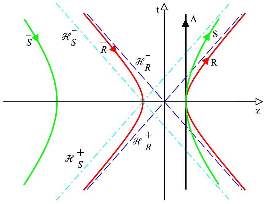
Consider three observers, Alice, Rob and Steven, such that Alice is at rest in an inertial frame, but Rob and Steven are moving with uniform accelerations with respect to Alice. We assign accelerations a1a_{1} and a2a_{2} to Steven and Rob, respectively. Fig. 1 shows the corresponding spacetime diagram. We see that at some points Alice’s signals will no longer reach to Rob and Steven, however, Rob’s and Steven’s signals will always reach to Alice. Each observer carries a detector sensitive only to a single mode of a fermionic field, kAk_{\textrm{A}} for Alice, kRk_{\textrm{R}} for Rob and kSk_{\textrm{S}} for Steven. We suppose a GHZ entanglement for this tripartite system, as viewed in an inertial frame. Therefore, we use the Minkowski modes to construct a GHZ state for the system as

|GHZ⟩ARSℳ=12​(|0kA⟩+​|0kR⟩+​|0kS⟩++|1kA⟩+​|1kR⟩+​|1kS⟩+).|\textrm{GHZ}\rangle^{\mathcal{M}}_{\textrm{ARS}}=\frac{1}{\sqrt{2}}\left(|0_{k_{\textrm{A}}}\rangle^{+}|0_{k_{\textrm{R}}}\rangle^{+}|0_{k_{\textrm{S}}}\rangle^{+}+|1_{k_{\textrm{A}}}\rangle^{+}|1_{k_{\textrm{R}}}\rangle^{+}|1_{k_{\textrm{S}}}\rangle^{+}\right). (6)

where we have used this fact that in a fermionic field there are only two allowed states for each Minkowski mode.
Refer to caption
Figure 1: Rindler spacetime diagram for an inertial observer Alice and two accelerated observers Rob and Steven. The thick black line shows the word line of Alice (A). A uniformly accelerated observer Rob (R) with acceleration a1a_{1} travels on a hyperbolic world line constrained to region I, and a fictitious observer anti-Rob (R¯)(\bar{\textrm{R}}) travels on the corresponding hyperbola in region II given by the negative of Rob’s coordinates (two thick red hyperbola). The horizons of R (R¯)(\bar{\textrm{R}}) are lines of τ=±∞\tau=\pm\infty which Alice (A) will cross them at finite Minkowski times corresponding to ℋR±\mathcal{H}^{\pm}_{R} (two dashed blue lines). Another uniformly accelerated observer Steven (S) travels on another hyperbola with an acceleration a2a_{2} constrained to region I′\textrm{I}^{\prime}, and a fictitious observer anti-Steven (S¯)(\bar{\textrm{S}}) travels on the corresponding hyperbola in region II′\textrm{II}^{\prime} given by the negative of Steven’s coordinates (two thick green hyperbola). The horizons of S (S¯)(\bar{\textrm{S}}), are lines of τ′=±∞\tau^{\prime}=\pm\infty which Alice (A) will cross them at finite Minkowski times, are ℋS±\mathcal{H}^{\pm}_{S} (two dashed cyan lines).

Now, we need to express the states |nkR⟩+|n_{k_{\textrm{R}}}\rangle^{+} and |nkS⟩+|n_{k_{\textrm{S}}}\rangle^{+}, in terms of Rindler states corresponding to Rob and Steven. Then using (4), we obtain

|GHZ⟩ARS\displaystyle|\textrm{GHZ}\rangle_{\textrm{ARS}} =\displaystyle= 12[|0kA⟩+(cosu1|0kR⟩I+|0−kR⟩II−+sinu1|1kR⟩I+|1−kR⟩II−)(cosu2|0kS⟩I′+|0−kS⟩II′−\displaystyle\frac{1}{\sqrt{2}}\left[|0_{k_{\textrm{A}}}\rangle^{+}(\cos u_{1}|0_{k_{\textrm{R}}}\rangle^{+}_{\textrm{I}}|0_{-k_{\textrm{R}}}\rangle^{-}_{\textrm{II}}+\sin u_{1}|1_{k_{\textrm{R}}}\rangle^{+}_{\textrm{I}}|1_{-k_{\textrm{R}}}\rangle^{-}_{\textrm{II}})(\cos u_{2}|0_{k_{\textrm{S}}}\rangle^{+}_{\textrm{I}^{\prime}}|0_{-k_{S}}\rangle^{-}_{\textrm{II}^{\prime}}\right. (7)
+sinu2|1kS⟩I′+|1−kS⟩II′−)+|1kA⟩+(|1kS⟩I+|0−kS⟩II−)(|1kS⟩I′+|0−kS⟩II′−)],\displaystyle\left.+\sin u_{2}|1_{k_{\textrm{S}}}\rangle^{+}_{I^{\prime}}|1_{-k_{\textrm{S}}}\rangle^{-}_{\textrm{II}^{\prime}})+|1_{k_{\textrm{A}}}\rangle^{+}(|1_{k_{\textrm{S}}}\rangle^{+}_{\textrm{I}}|0_{-k_{\textrm{S}}}\rangle^{-}_{\textrm{II}})(|1_{k_{\textrm{S}}}\rangle^{+}_{\textrm{I}^{\prime}}|0_{-k_{\textrm{S}}}\rangle^{-}_{\textrm{II}^{\prime}})\right],

where |nkR⟩I+|n_{k_{\textrm{R}}}\rangle^{+}_{\textrm{I}} (or |nkS⟩I′+|n_{k_{\textrm{S}}}\rangle^{+}_{\textrm{I}^{\prime}}) is the Rindler-region-I-particle mode for Rob (or Steven), |n−kR⟩II−|n_{-k_{\textrm{R}}}\rangle^{-}_{\textrm{II}} (or |n−kS⟩II′−|n_{-k_{\textrm{S}}}\rangle^{-}_{\textrm{II}^{\prime}}) is Rindler-region-II-antiparticle mode for Rob (or Steven), and tanui=exp(−πωc/ai)\tan u_{i}=\exp(-\pi\omega c/a_{i}) with i∈{1,2}i\in\{1,2\}.

Using the basis {|nkA⟩+​|nkR⟩+​|nkS⟩+}\{|n_{k_{\textrm{A}}}\rangle^{+}|n_{k_{\textrm{R}}}\rangle^{+}|n_{k_{\textrm{S}}}\rangle^{+}\} that is {|000⟩,|001⟩,|010⟩,|100⟩,|011⟩,|101⟩,|110⟩,|111⟩}\{|000\rangle,|001\rangle,|010\rangle,|100\rangle,|011\rangle,|101\rangle,|110\rangle,|111\rangle\}, we can obtain the density matrix for the GHZ state (6) as

ρARSℳ\displaystyle\rho^{\mathcal{M}}_{\textrm{ARS}} =\displaystyle= 18​(Σ1⊗Σ1⊗Σ1−Σ1⊗Σ2⊗Σ2−Σ2⊗Σ1⊗Σ2−Σ2⊗Σ2⊗Σ1CLOSE\displaystyle\frac{1}{8}\left(\Sigma_{1}\otimes\Sigma_{1}\otimes\Sigma_{1}-\Sigma_{1}\otimes\Sigma_{2}\otimes\Sigma_{2}-\Sigma_{2}\otimes\Sigma_{1}\otimes\Sigma_{2}-\Sigma_{2}\otimes\Sigma_{2}\otimes\Sigma_{1}\right. (8)
+Σ3⊗Σ3⊗I+Σ3⊗I⊗Σ3+I⊗Σ3⊗Σ3+I⊗I⊗I)\displaystyle\left.+\Sigma_{3}\otimes\Sigma_{3}\otimes I+\Sigma_{3}\otimes I\otimes\Sigma_{3}+I\otimes\Sigma_{3}\otimes\Sigma_{3}+I\otimes I\otimes I\right)

where II is the unit 2×22\times 2 matrix and {Σ1,Σ2,Σ3}\{\Sigma_{1},\Sigma_{2},\Sigma_{3}\} are the Pauli matrices. Notice that here and in the following, the matrices in each tensor product term are placed according to Alice-Rob-Steven order. The pure state (8) describes a tripartite system. On the other hand, the density matrix for the state (9) is obtained as ρA,I,I′,II,II′=|GHZ⟩ARS​⟨GHZ|\rho_{\textrm{A},\textrm{I},\textrm{I}^{\prime},\textrm{II},\textrm{II}^{\prime}}=|\textrm{GHZ}\rangle_{\textrm{ARS}}\langle\textrm{GHZ}|, which is pure and describes a five-partite system. However, as Fig. 1 represents, whole of spacetime is accessible only for the inertial observer Alice, and the accelerating observer Rob (or Steven) has only access to one region say I (or I′\textrm{I}^{\prime}). So, we must trace over the states belong to regions II and II′\textrm{II}^{\prime}. Doing so, we get the following tripartite density matrix

ρA,I,I′\displaystyle\rho_{\textrm{A},\textrm{I},\textrm{I}^{\prime}} =\displaystyle= 18[cosu1cosu2(Σ1⊗Σ1⊗Σ1−Σ1⊗Σ2⊗Σ2−Σ2⊗Σ1⊗Σ2\displaystyle\frac{1}{8}\left[\cos{u_{1}}\cos{u_{2}}(\Sigma_{1}\otimes\Sigma_{1}\otimes\Sigma_{1}-\Sigma_{1}\otimes\Sigma_{2}\otimes\Sigma_{2}-\Sigma_{2}\otimes\Sigma_{1}\otimes\Sigma_{2}\right. (9)
−Σ2⊗Σ2⊗Σ1)+12(cos2u1cos2u2−1)(Σ3⊗Σ3⊗Σ3)+cos2u1(Σ3⊗Σ3⊗I)\displaystyle\left.-\Sigma_{2}\otimes\Sigma_{2}\otimes\Sigma_{1})+\frac{1}{2}(\cos{2u_{1}}\cos{2u_{2}}-1)(\Sigma_{3}\otimes\Sigma_{3}\otimes\Sigma_{3})+\cos^{2}{u_{1}}(\Sigma_{3}\otimes\Sigma_{3}\otimes I)\right.
+cos2⁡u2​(Σ3⊗I⊗Σ3)+12​(cos⁡2​u1​cos⁡2​u2+1)​(I⊗Σ3⊗Σ3)−sin2⁡u1​(I⊗Σ3⊗I)\displaystyle\left.+\cos^{2}u_{2}(\Sigma_{3}\otimes I\otimes\Sigma_{3})+\frac{1}{2}(\cos{2u_{1}}\cos{2u_{2}}+1)(I\otimes\Sigma_{3}\otimes\Sigma_{3})-\sin^{2}u_{1}(I\otimes\Sigma_{3}\otimes I)\right.
−sin2u2(I⊗I⊗Σ3)+I⊗I⊗I]\displaystyle\left.-\sin^{2}u_{2}(I\otimes I\otimes\Sigma_{3})+I\otimes I\otimes I\right]

where we have employed the basis {|nkA⟩+​|nkR⟩I+​|nkS⟩I′+}\{|n_{k_{\textrm{A}}}\rangle^{+}|n_{k_{\textrm{R}}}\rangle^{+}_{\textrm{I}}|n_{k_{\textrm{S}}}\rangle^{+}_{\textrm{I}^{\prime}}\}. While the state (8) is pure and maximally entangled, the state (9) is not pure and, as we will verify, its entanglement is degraded. This entanglement degradation is essentially justified by the Unruh effect.

III.1.1 A-RS, R-AS, S-AR entanglements

To quantify the entanglement in a tripartite system, different measures have been introduced. Here, regarding the dimension of the density matrix (9) and that the state is not pure, we consider the logarithmic negativity which describes the entanglement of one part of the system relative to the other parts. For instance, the logarithmic negativity of Alice part relative to the other two parts is defined as 𝒩A−RS=∑ilog2⁡|λi|\mathcal{N}_{\textrm{A}-\textrm{RS}}=\sum_{i}\log_{2}|\lambda_{i}| where λi\lambda_{i} denotes the eigenvalues of ρA~,I,I′\rho_{\widetilde{\textrm{A}},\textrm{I},\textrm{I}^{\prime}} which is the partial transposition of ρA,I,I′\rho_{\textrm{A},\textrm{I},\textrm{I}^{\prime}} with respect to Alice. Similarly, we can calculate 𝒩R−AS\mathcal{N}_{\textrm{R}-\textrm{AS}} and 𝒩S−AR\mathcal{N}_{\textrm{S}-\textrm{AR}} by finding the eigenvalues of ρA,I~,I′\rho_{\textrm{A},\widetilde{\textrm{I}},\textrm{I}^{\prime}} (partially transposed density matrix with respect to Rob) and ρA,I,I′~\rho_{\textrm{A},\textrm{I},\widetilde{\textrm{I}^{\prime}}} (partially transposed density matrix with respect to Steven). Logarithmic Negativity vanishes unless some negative eigenvalues are present. Let NN denote the negative eigenvalue, then we can write the logarithmic negativity also as

𝒩=log2⁡(1−2​N)\mathcal{N}=\log_{2}(1-2N) (10)

We can readily obtain the required partially transposed matrices from (9) by noting that after a transposition, Σ1\Sigma_{1} and Σ3\Sigma_{3} do not change but Σ2⟶−Σ2\Sigma_{2}\longrightarrow-\Sigma_{2}. We have

ρA~,I,I′=ϱ−18cosu1cosu2(Σ1⊗Σ2⊗Σ2−Σ2⊗Σ1⊗Σ2−Σ2⊗Σ2⊗Σ1),\rho_{\widetilde{\textrm{A}},\textrm{I},\textrm{I}^{\prime}}=\varrho-\frac{1}{8}\cos{u_{1}}\cos{u_{2}}(\Sigma_{1}\otimes\Sigma_{2}\otimes\Sigma_{2}-\Sigma_{2}\otimes\Sigma_{1}\otimes\Sigma_{2}-\Sigma_{2}\otimes\Sigma_{2}\otimes\Sigma_{1}), (11)
ρA,I~,I′=ϱ−18cosu1cosu2(−Σ1⊗Σ2⊗Σ2+Σ2⊗Σ1⊗Σ2−Σ2⊗Σ2⊗Σ1),\rho_{\textrm{A},\widetilde{\textrm{I}},\textrm{I}^{\prime}}=\varrho-\frac{1}{8}\cos{u_{1}}\cos{u_{2}}(-\Sigma_{1}\otimes\Sigma_{2}\otimes\Sigma_{2}+\Sigma_{2}\otimes\Sigma_{1}\otimes\Sigma_{2}-\Sigma_{2}\otimes\Sigma_{2}\otimes\Sigma_{1}), (12)

and

ρA,I,I′~=ϱ−18cosu1cosu2(−Σ1⊗Σ2⊗Σ2−Σ2⊗Σ1⊗Σ2+Σ2⊗Σ2⊗Σ1),\rho_{\textrm{A},\textrm{I},\widetilde{\textrm{I}^{\prime}}}=\varrho-\frac{1}{8}\cos{u_{1}}\cos{u_{2}}(-\Sigma_{1}\otimes\Sigma_{2}\otimes\Sigma_{2}-\Sigma_{2}\otimes\Sigma_{1}\otimes\Sigma_{2}+\Sigma_{2}\otimes\Sigma_{2}\otimes\Sigma_{1}), (13)

where

ϱ\displaystyle\varrho =\displaystyle= 18[cosu1cosu2(Σ1⊗Σ1⊗Σ1)+12(cos2u1cos2u2−1)(Σ3⊗Σ3⊗Σ3)\displaystyle\frac{1}{8}\left[\cos{u_{1}}\cos{u_{2}}(\Sigma_{1}\otimes\Sigma_{1}\otimes\Sigma_{1})+\frac{1}{2}(\cos{2u_{1}}\cos{2u_{2}}-1)(\Sigma_{3}\otimes\Sigma_{3}\otimes\Sigma_{3})\right. (14)
+cos2⁡u1​(Σ3⊗Σ3⊗I)+cos2⁡u2​(Σ3⊗I⊗Σ3)+12​(cos⁡2​u1​cos⁡2​u2+1)​(I⊗Σ3⊗Σ3)\displaystyle\left.+\cos^{2}{u_{1}}(\Sigma_{3}\otimes\Sigma_{3}\otimes I)+\cos^{2}u_{2}(\Sigma_{3}\otimes I\otimes\Sigma_{3})+\frac{1}{2}(\cos{2u_{1}}\cos{2u_{2}}+1)(I\otimes\Sigma_{3}\otimes\Sigma_{3})\right.
−sin2u1(I⊗Σ3⊗I)−sin2u2(I⊗I⊗Σ3)+I⊗I⊗I].\displaystyle\left.-\sin^{2}u_{1}(I\otimes\Sigma_{3}\otimes I)-\sin^{2}u_{2}(I\otimes I\otimes\Sigma_{3})+I\otimes I\otimes I\right].

The eigenvalues of each of these partially transposed matrices can be obtained explicitly, however, we need only negative eigenvalues. It turns out that the negative eigenvalues for (11), (12) and (13) are

NA-RS=14​sin2⁡u1​sin2⁡u2−14​sin4⁡u1​sin4⁡u2+4​cos2⁡u1​cos2⁡u2,N_{\textrm{A-RS}}=\frac{1}{4}\sin^{2}u_{1}\sin^{2}u_{2}-\frac{1}{4}\,\sqrt{\sin^{4}u_{1}\sin^{4}u_{2}+4\cos^{2}u_{1}\cos^{2}u_{2}}, (15)
NR-AS=14​sin2⁡u1​cos2⁡u2−14​sin4⁡u1​cos4⁡u2+4​cos2⁡u1​cos2⁡u2,N_{\textrm{R-AS}}=\frac{1}{4}\sin^{2}u_{1}\cos^{2}u_{2}-\frac{1}{4}\,\sqrt{\sin^{4}u_{1}\cos^{4}u_{2}+4\cos^{2}u_{1}\cos^{2}u_{2}}, (16)

and

NS-AR=14​sin2⁡u2​cos2⁡u1−14​sin4⁡u2​cos4⁡u1+4​cos2⁡u2​cos2⁡u1,N_{\textrm{S-AR}}=\frac{1}{4}\sin^{2}u_{2}\cos^{2}u_{1}-\frac{1}{4}\,\sqrt{\sin^{4}u_{2}\cos^{4}u_{1}+4\cos^{2}u_{2}\cos^{2}u_{1}}, (17)

respectively. For investigating the entanglement, we substitute these eigenvalues in (10) to obtain the corresponding logarithmic negativity as functions of u1u_{1} and u2u_{2}. Recall that in the present case 0≤ui<π40\leq u_{i}<\frac{\pi}{4} corresponding to 0≤ai<∞0\leq a_{i}<\infty where aia_{i} indicates the proper acceleration of Rob or Steven. We have plotted all three surfaces 𝒩R−AS\mathcal{N}_{\textrm{R}-\textrm{AS}}, 𝒩S−AR\mathcal{N}_{\textrm{S}-\textrm{AR}} and 𝒩A−RS\mathcal{N}_{\textrm{A}-\textrm{RS}} in Fig. 2(a). Each surface shows a uniform decreasing of logarithmic negativity as accelerations increase. It must be noted that even for infinite accelerations, that is, u1,u2→π4u_{1},u_{2}\rightarrow\frac{\pi}{4}, each logarithmic negativity does not vanish. In other words, like bipartite entanglement, the Unruh effect doesn’t completely destroy the entanglement. We see that the surface of 𝒩A−RS\mathcal{N}_{\textrm{A}-\textrm{RS}} covers the other two surfaces. To illustrate the situation a section of Fig. 2(a) for a given u2=3​π/16u_{2}=3\pi/16 is plotted in Fig. 2. It is remarkable that these entanglements are not generally equal. This means that in the considered tripartite system each part is differently entangled to the other two parts; the inertial Alice part is mostly entangled. Of course, the surfaces of 𝒩R−AS\mathcal{N}_{\textrm{R}-\textrm{AS}} and 𝒩S−AR\mathcal{N}_{\textrm{S}-\textrm{AR}} intersect at u1=u2u_{1}=u_{2}, i.e., when Rob and Steven have the same acceleration, have the same entanglement, expectedly.

Refer to caption
(a)
Refer to caption
Figure 2: Logarithmic negativity for the fermionic GHZ state versus accelerations u1u_{1} and u2u_{2}. (a) The two lower surfaces that intersect at u1=u2u_{1}=u_{2}, represent 𝒩R−AS\mathcal{N}_{\textrm{R}-\textrm{AS}} and 𝒩S−AR\mathcal{N}_{\textrm{S}-\textrm{AR}}. The upper surface corresponds to 𝒩A−RS\mathcal{N}_{\textrm{A}-\textrm{RS}}. (b) A section of figure (a) for a given u2=3​π/16u_{2}=3\pi/16. Even for infinite accelerations or u1,u2→π4u_{1},u_{2}\rightarrow\frac{\pi}{4}, each logarithmic negativity does not vanish, i.e., the Unruh effect does not completely destroy the entanglement in this case.

III.1.2 Entanglement of bipartite subsystems

In this subsection, we attend to the entanglement of bipartite subsystems AR, AS and RS. To do this, we must trace out one of the parts of the tripartite system ARS described by the density matrix (9). We can readily trace over Alice, Rob or Steven states by noting that the Pauli matrices are traceless. For instance, upon tracing over the Alice states, only the tensor product terms remain where the first matrix is the unity matrix II. Then, we obtain the following reduced density matrix for RS subsystem

ρI,I′=14​[12​(cos⁡2​u1​cos⁡2​u2+1)​(Σ3⊗Σ3)−sin2⁡u1​(Σ3⊗I)−sin2⁡u2​(I⊗Σ3)+I⊗I],\rho_{\textrm{I},\textrm{I}^{\prime}}=\frac{1}{4}\left[\frac{1}{2}(\cos{2u_{1}}\cos{2u_{2}}+1)(\Sigma_{3}\otimes\Sigma_{3})-\sin^{2}u_{1}(\Sigma_{3}\otimes I)-\sin^{2}u_{2}(I\otimes\Sigma_{3})+I\otimes I\right], (18)

which is diagonal. In the same manner we see that the reduced density matrices for AR and AS subsystems are also diagonal. Thus, each of these bipartite subsystems is disentangled. This means that the GHZ character of the state is preserved under the Unruh effect, that is, tracing over any part of a GHZ state, leads to a disentangled bipartite subsystem [19].

III.2 The W state

In this subsection we assume a W entanglement for the tripartite system ARS as viewed in an inertial frame. Therefor, we use the Minkowski modes to construct a W state as

|W⟩ARSℳ=13​(|1kA⟩+​|0kR⟩+​|0kS⟩++|0kA⟩+​|1kR⟩+​|0kS⟩++|0kA⟩+​|0kR⟩+​|1kS⟩+).|\textrm{W}\rangle^{\mathcal{M}}_{\textrm{ARS}}=\frac{1}{\sqrt{3}}\left(|1_{k_{\textrm{A}}}\rangle^{+}|0_{k_{\textrm{R}}}\rangle^{+}|0_{k_{\textrm{S}}}\rangle^{+}+|0_{k_{\textrm{A}}}\rangle^{+}|1_{k_{\textrm{R}}}\rangle^{+}|0_{k_{\textrm{S}}}\rangle^{+}+|0_{k_{\textrm{A}}}\rangle^{+}|0_{k_{\textrm{R}}}\rangle^{+}|1_{k_{\textrm{S}}}\rangle^{+}\right). (19)

The corresponding density matrix for this state is obtained as

ρARSℳ\displaystyle\rho^{\mathcal{M}}_{\textrm{ARS}} =\displaystyle= 124[2(Σ1⊗Σ1⊗Σ3+Σ2⊗Σ2⊗Σ3+Σ1⊗Σ3⊗Σ1+Σ2⊗Σ3⊗Σ2\displaystyle\frac{1}{24}\left[2(\Sigma_{1}\otimes\Sigma_{1}\otimes\Sigma_{3}+\Sigma_{2}\otimes\Sigma_{2}\otimes\Sigma_{3}+\Sigma_{1}\otimes\Sigma_{3}\otimes\Sigma_{1}+\Sigma_{2}\otimes\Sigma_{3}\otimes\Sigma_{2}\right. (20)
+Σ3⊗Σ1⊗Σ1+Σ3⊗Σ2⊗Σ2+Σ1⊗I⊗Σ1+Σ1⊗Σ1⊗I+Σ2⊗Σ2⊗I\displaystyle\left.+\Sigma_{3}\otimes\Sigma_{1}\otimes\Sigma_{1}+\Sigma_{3}\otimes\Sigma_{2}\otimes\Sigma_{2}+\Sigma_{1}\otimes I\otimes\Sigma_{1}+\Sigma_{1}\otimes\Sigma_{1}\otimes I+\Sigma_{2}\otimes\Sigma_{2}\otimes I\right.
+Σ2⊗I⊗Σ2+I⊗Σ1⊗Σ1+I⊗Σ2⊗Σ2)−3(Σ3⊗Σ3⊗Σ3)−Σ3⊗I⊗Σ3\displaystyle\left.+\Sigma_{2}\otimes I\otimes\Sigma_{2}+I\otimes\Sigma_{1}\otimes\Sigma_{1}+I\otimes\Sigma_{2}\otimes\Sigma_{2})-3(\Sigma_{3}\otimes\Sigma_{3}\otimes\Sigma_{3})-\Sigma_{3}\otimes I\otimes\Sigma_{3}\right.
−I⊗Σ3⊗Σ3−Σ3⊗Σ3⊗I+Σ3⊗I⊗I+I⊗Σ3⊗I+I⊗I⊗Σ3+3(I⊗I⊗I)].\displaystyle\left.-I\otimes\Sigma_{3}\otimes\Sigma_{3}-\Sigma_{3}\otimes\Sigma_{3}\otimes I+\Sigma_{3}\otimes I\otimes I+I\otimes\Sigma_{3}\otimes I+I\otimes I\otimes\Sigma_{3}+3(I\otimes I\otimes I)\right].

Then we apply the Bogoliubov transformation (4) for the accelerating observers Rob and Steven and rewrite the state (19) in Rindler coordinates which leads to a density matrix describing a five-partite system. After tracing over the causally disconnected regions II and II′\textrm{II}^{\prime}, we reach to

ρA,I,I′\displaystyle\rho_{\textrm{A},\textrm{I},\textrm{I}^{\prime}} =\displaystyle= 124[2cosu1cos2u2(Σ1⊗Σ1⊗Σ3+Σ2⊗Σ2⊗Σ3)+2cosu2(Σ1⊗I⊗Σ1+Σ2⊗I⊗Σ2)\displaystyle\frac{1}{24}\left[2\cos{u_{1}}\cos{2u_{2}}(\Sigma_{1}\otimes\Sigma_{1}\otimes\Sigma_{3}+\Sigma_{2}\otimes\Sigma_{2}\otimes\Sigma_{3})+2\cos{u_{2}}(\Sigma_{1}\otimes I\otimes\Sigma_{1}+\Sigma_{2}\otimes I\otimes\Sigma_{2})\right. (21)
+2cosu1(Σ1⊗Σ1⊗I+Σ2⊗Σ2⊗I)+2cos2u1cosu2(Σ1⊗Σ3⊗Σ1+Σ2⊗Σ3⊗Σ2)\displaystyle\left.+2\cos{u_{1}}(\Sigma_{1}\otimes\Sigma_{1}\otimes I+\Sigma_{2}\otimes\Sigma_{2}\otimes I)+2\cos{2u_{1}}\cos{u_{2}}(\Sigma_{1}\otimes\Sigma_{3}\otimes\Sigma_{1}+\Sigma_{2}\otimes\Sigma_{3}\otimes\Sigma_{2})\right.
+2cosu1cosu2(Σ3⊗Σ1⊗Σ1+Σ3⊗Σ2⊗Σ2+I⊗Σ1⊗Σ1+I⊗Σ2⊗Σ2)\displaystyle\left.+2\cos{u_{1}}\cos{u_{2}}(\Sigma_{3}\otimes\Sigma_{1}\otimes\Sigma_{1}+\Sigma_{3}\otimes\Sigma_{2}\otimes\Sigma_{2}+I\otimes\Sigma_{1}\otimes\Sigma_{1}+I\otimes\Sigma_{2}\otimes\Sigma_{2})\right.
−(cos⁡2​u1​cos⁡2​u2+cos⁡2​u1+cos⁡2​u2)​(Σ3⊗Σ3⊗Σ3)−Σ3⊗Σ3⊗I−Σ3⊗I⊗Σ3+Σ3⊗I⊗I\displaystyle\left.-(\cos 2u_{1}\cos 2u_{2}+\cos 2{u_{1}}+\cos 2{u_{2}})(\Sigma_{3}\otimes\Sigma_{3}\otimes\Sigma_{3})-\Sigma_{3}\otimes\Sigma_{3}\otimes I-\Sigma_{3}\otimes I\otimes\Sigma_{3}+\Sigma_{3}\otimes I\otimes I\right.
+(cos⁡2​u1​cos⁡2​u2−cos⁡2​u1−cos⁡2​u2)​(I⊗Σ3⊗Σ3)+(2​cos⁡2​u1−1)​(I⊗Σ3⊗I)\displaystyle\left.+(\cos 2u_{1}\cos 2u_{2}-\cos 2u_{1}-\cos 2u_{2})(I\otimes\Sigma_{3}\otimes\Sigma_{3})+(2\cos 2{u_{1}}-1)(I\otimes\Sigma_{3}\otimes I)\right.
+(2cos2u2−1)(I⊗I⊗Σ3)+3(I⊗I⊗I)]\displaystyle\left.+(2\cos 2{u_{2}}-1)(I\otimes I\otimes\Sigma_{3})+3(I\otimes I\otimes I)\right]

III.2.1 A-RS, R-AS and S-AR entanglements

Again we want to use the logarithmic negativity given by (10) for evaluating the entanglement of the state (21). To do this we first obtain the partially transposed matrices ρA~,I,I′\rho_{\widetilde{\textrm{A}},\textrm{I},\textrm{I}^{\prime}},ρA,I~,I′\rho_{\textrm{A},\widetilde{\textrm{I}},\textrm{I}^{\prime}} and ρA,I,I′~\rho_{\textrm{A},\textrm{I},\widetilde{\textrm{I}^{\prime}}}. Then we must calculate the negative eigenvalues for them and substitute in (10). However, these calculations are lengthy and here we only present the results by plotting the obtained logarithmic negativity in Fig. 3. These surfaces show the logarithmic negativity in term of accelerations u1u_{1} and u2u_{2}. We see that the surface of 𝒩A−RS\mathcal{N}_{\textrm{A}-\textrm{RS}} lies below of the surfaces of 𝒩R−AS\mathcal{N}_{\textrm{R}-\textrm{AS}} and 𝒩S−AR\mathcal{N}_{\textrm{S}-\textrm{AR}}, and is covered by them when u1u_{1} and u2u_{2} take their full range. Fig. (3) represent the situation more clearly. As is seen, again in the considered system each part is entangled differently. Expectedly, the surfaces 𝒩R−AS\mathcal{N}_{\textrm{R}-\textrm{AS}} and 𝒩S−AR\mathcal{N}_{\textrm{S}-\textrm{AR}} intersect at u1=u2u_{1}=u_{2}. However, it is interesting to note that the surface 𝒩A−RS\mathcal{N}_{\textrm{A}-\textrm{RS}} intersects the 𝒩R−AS\mathcal{N}_{\textrm{R}-\textrm{AS}} and 𝒩S−AR\mathcal{N}_{\textrm{S}-\textrm{AR}} at definite values of u1u_{1} and u2u_{2}, i.e., in the considered W state, for definite accelerations the entanglement of part R or S can be equal to the entanglement of inertial part A. Note that similar to the GHZ case discussed in the previous subsection, some degree of W entanglement is preserved as a1a_{1} and a2a_{2} go to infinity. This result is obtained also for fermionic bipartite entanglement and has been proven to be universal for fermionic fields [15].

Refer to caption
Refer to caption
Refer to caption
Figure 3: Logarithmic negativity for the fermionic W state versus accelerations u1u_{1} and u2u_{2}. (a) The surface 𝒩A−RS\mathcal{N}_{\textrm{A}-\textrm{RS}} in terms of u1u_{1} and u2u_{2}. (b) 𝒩A−RS\mathcal{N}_{\textrm{A}-\textrm{RS}}, 𝒩R−AS\mathcal{N}_{\textrm{R}-\textrm{AS}} and 𝒩S−AR\mathcal{N}_{\textrm{S}-\textrm{AR}} surfaces all together. Again 𝒩R−AS\mathcal{N}_{\textrm{R}-\textrm{AS}} and 𝒩S−AR\mathcal{N}_{\textrm{S}-\textrm{AR}} surfaces intersect along u1=u2u_{1}=u_{2}. The surface of 𝒩A−RS\mathcal{N}_{\textrm{A}-\textrm{RS}} is not seen here , because, this lies below the other two surfaces. (c) A section of the figure (b) for a given u2=π/8u_{2}=\pi/8. The surface 𝒩A−RS\mathcal{N}_{\textrm{A}-\textrm{RS}} intersects 𝒩R−AS\mathcal{N}_{\textrm{R}-\textrm{AS}} or 𝒩S−AR\mathcal{N}_{\textrm{S}-\textrm{AR}} at determined values of u1u_{1} and u2u_{2}. Like the GHZ case, even for infinite values of a1a_{1} and a2a_{2}, the logarithmic negativity generally is nonzero.

III.2.2 Entanglement of bipartite subsystems

Let us study the entanglement of bipartite subsystems AR, AS and RS, by tracing over the states of one of the parts of the tripartite system described by (21). We denote the resulting density matrices as ρI,I′\rho_{\textrm{I},\textrm{I}^{\prime}}, ρA,I\rho_{\textrm{A},\textrm{I}} and ρA,I′\rho_{\textrm{A},\textrm{I}^{\prime}}, when we trace over Alice, Steven and Rob, respectively. We readily obtain from (21)

ρI,I′\displaystyle\rho_{\textrm{I},\textrm{I}^{\prime}} =\displaystyle= 112[2cosu1cosu2(Σ1⊗Σ1+Σ2⊗Σ2)+(cos2u1cos2u2−cos2u1−cos2u2)(Σ3⊗Σ3)\displaystyle\frac{1}{12}\left[2\cos{u_{1}}\cos{u_{2}}(\Sigma_{1}\otimes\Sigma_{1}+\Sigma_{2}\otimes\Sigma_{2})+(\cos 2u_{1}\cos 2u_{2}-\cos 2u_{1}-\cos 2u_{2})(\Sigma_{3}\otimes\Sigma_{3})\right. (22)
+(2cos2u1−1)(Σ3⊗I)+(2cos2u2−1)(I⊗Σ3)+3(I⊗I)],\displaystyle\left.+(2\cos 2u_{1}-1)(\Sigma_{3}\otimes I)+(2\cos 2u_{2}-1)(I\otimes\Sigma_{3})+3(I\otimes I)\right],
ρA,I\displaystyle\rho_{\textrm{A},\textrm{I}} =\displaystyle= 112[2cosu1(Σ1⊗Σ1+Σ2⊗Σ2)−Σ3⊗Σ3+Σ3⊗I\displaystyle\frac{1}{12}\left[2\cos{u_{1}}(\Sigma_{1}\otimes\Sigma_{1}+\Sigma_{2}\otimes\Sigma_{2})-\Sigma_{3}\otimes\Sigma_{3}+\Sigma_{3}\otimes I\right. (23)
+(2cos2u1−1)(I⊗Σ3)+3(I⊗I)],\displaystyle+\left.(2\cos 2u_{1}-1)(I\otimes\Sigma_{3})+3(I\otimes I)\right],

and

ρA,I′\displaystyle\rho_{\textrm{A},\textrm{I}^{\prime}} =\displaystyle= 112[2cosu2(Σ1⊗Σ1+Σ2⊗Σ2)−Σ3⊗Σ3+Σ3⊗I\displaystyle\frac{1}{12}\left[2\cos{u_{2}}(\Sigma_{1}\otimes\Sigma_{1}+\Sigma_{2}\otimes\Sigma_{2})-\Sigma_{3}\otimes\Sigma_{3}+\Sigma_{3}\otimes I\right. (24)
+(2cos2u2−1)(I⊗Σ3)+3(I⊗I)],\displaystyle+\left.(2\cos 2u_{2}-1)(I\otimes\Sigma_{3})+3(I\otimes I)\right],

In contrast to the GHZ case, these bipartite subsystems are not disentangled. We can still use the logarithmic negativity (10) for calculating these bipartite entanglements. To do this we must first find the negative eigenvalues for partially transposed matrices ρI~,I′\rho_{\widetilde{\textrm{I}},\textrm{I}^{\prime}}, ρA~,I\rho_{\widetilde{\textrm{A}},\textrm{I}} and ρA~,I\rho_{\widetilde{\textrm{A}},\textrm{I}} corresponding to the above matrices. We obtain

NRS\displaystyle N_{\textrm{R}\textrm{S}} =\displaystyle= 12−13(cos2u1+cos2u2)+13(cosu1cosu2)2\displaystyle\frac{1}{2}-\frac{1}{3}(\cos^{2}u_{1}+\cos^{2}u_{2})+\frac{1}{3}(\cos u_{1}\cos u_{2})^{2} (25)
−16​9−12(cos2u1+cos2u2)+12(cosu1cosu2)2+4(cos4u1+cos4u2),\displaystyle-\frac{1}{6}\sqrt{9-12(\cos^{2}u_{1}+\cos^{2}u_{2})+12(\cos u_{1}\cos u_{2})^{2}+4(\cos^{4}u_{1}+\cos^{4}u_{2})},
NAR=16−16​1+4​cos4⁡u2,N_{\textrm{A}\textrm{R}}=\frac{1}{6}-\frac{1}{6}\,\sqrt{1+4\,\cos^{4}u_{2}}, (26)
NAS=16−16​1+4​cos4⁡u1,N_{\textrm{A}\textrm{S}}=\frac{1}{6}-\frac{1}{6}\,\sqrt{1+4\,\cos^{4}u_{1}}, (27)

which as substituted in (10), give the corresponding logarithmic negativity. It is remarkable that the negativity NRSN_{\textrm{R}\textrm{S}} in (25) and consequently the logarithmic negativity 𝒩RS\mathcal{N}_{\textrm{R}\textrm{S}} vanish if u1u_{1} and u2u_{2} satisfy the equation

cos⁡u2=2sinu12−cos2⁡u1.\cos u_{2}=\frac{\sqrt{2}\sin u_{1}}{\sqrt{2-\cos^{2}u_{1}}}. (28)

Fig. 4(a) shows the behavior of 𝒩RS\mathcal{N}_{\textrm{R}\textrm{S}} in terms of u1u_{1} and u2u_{2}. We see that if the accelerations of Rob and Steven satisfy (28), the entanglement between them will be removed, completely. This is a remarkable result and it seems that this contradicts the general behavior of fermionic entanglements under the Unruh effect. However, 𝒩RS\mathcal{N}_{\textrm{R}\textrm{S}} represents the residual entanglement of Rob and Steven parties after tracing over the Alice states. Thus, the entanglement level for this system is lower than the entanglement of the whole tripartite system, as Fig. 4(a) shows. Moreover, both Rob and Steven are accelerated observers and so the rate of entanglement degradation is such that the entanglement descends to zero for finite accelerations.

In Fig. (4) we have plotted 𝒩AR\mathcal{N}_{\textrm{A}\textrm{R}} (𝒩AS\mathcal{N}_{\textrm{A}\textrm{S}}) which depends only on u1u_{1} (u2u_{2}). Since the entanglement is destroyed upon tracing over Steven (Rob), the curve starts with 0.50.5 at u1=0u_{1}=0 (u2=0u_{2}=0), as for RS subsystem. But, here only one of the observers accelerates and the entanglement degradation is not enough for vanishing the entanglement at a finite or even infinite acceleration.

It must be noted that after tracing out any part of the tripartite state (21) we obtain a bipartite subsystem having some residual entanglement, in an apparent contrast to the GHZ case. One may say that the Unruh effect does not change the class of the W state (19). Notice that a W state remains entangled after tracing out one of its parts. However, it is remarkable that for RS subsystem the residual entanglement can completely be removed for appropriate accelerations of Rob and Steven.

Refer to caption
(a)
Refer to caption
Figure 4: The logarithmic negativity versus u1u_{1} and u2u_{2} for bipartite subsystems when the tripartite system is in the fermionic W state. (a) 𝒩RS\mathcal{N}_{\textrm{R}\textrm{S}} surface which represents the entanglement of Rob and Steven states in their first regions I and I′\textrm{I}^{\prime}. As is seen, 𝒩RS\mathcal{N}_{\textrm{R}\textrm{S}} equals 0.50.5 at u1=u2=0u_{1}=u_{2}=0, then reaches to zero at a curve defined by (28). (b) 𝒩AR\mathcal{N}_{\textrm{A}\textrm{R}} (𝒩AS\mathcal{N}_{\textrm{A}\textrm{S}}) depends only on u1u_{1} (u2u_{2}). The curve starts with 0.50.5 at u1=0u_{1}=0 (u2=0u_{2}=0), then descends to a non-zero asymptotic value.

IV Bosonic entanglements

In this section we are going to discuss the effect of Unruh temperature on the bosonic tripartite GHZ and W entanglements. Because of the nature of bosonic states and hence the form of corresponding Bogoliubov transformation (5), our calculations will be more complicated than the calculations for the GHZ case discussed in the before section. We begin with the bosonic GHZ state.

IV.1 The GHZ state

Again we consider the GHZ state (6) which is written in terms of Minkowski modes. In the present argument we expand Minkowski states |0kR⟩+|0_{k_{\textrm{R}}}\rangle^{+} and |0kS⟩+|0_{k_{\textrm{S}}}\rangle^{+} in terms of Rindler bosonic states for Rob and Steven, using the Bogoliubov transformation (5). Then we can write

|GHZ⟩ARS\displaystyle|\textrm{GHZ}\rangle_{\textrm{ARS}} =\displaystyle= 12[|0⟩(1cosh⁡r1∑n∞tanhnr1|n⟩I|n⟩II)(1cosh⁡r2∑m∞tanhmr2|m⟩I′|n⟩II′)\displaystyle\frac{1}{\sqrt{2}}\left[|0\rangle\left(\frac{1}{\cosh{r_{1}}}\sum_{n}^{\infty}\tanh^{n}{r_{1}}|n\rangle_{\textrm{I}}|n\rangle_{\textrm{II}}\right)\left(\frac{1}{\cosh{r_{2}}}\sum_{m}^{\infty}\tanh^{m}{r_{2}}|m\rangle_{\textrm{I}^{\prime}}|n\rangle_{\textrm{II}^{\prime}}\right)\right. (30)
+|1⟩​(1cosh2⁡r1​∑n=0∞tanhn⁡r1​n+1​|n+1⟩I​|n⟩II)\displaystyle\left.+|1\rangle\left(\frac{1}{\cosh^{2}{r_{1}}}\sum_{n=0}^{\infty}\tanh^{n}{r_{1}}\sqrt{n+1}|n+1\rangle_{\textrm{I}}|n\rangle_{\textrm{II}}\right)\right.
×(1cosh2⁡r2∑m=0∞tanhmr2m+1|m+1⟩I′|m⟩II′)].\displaystyle\left.\times\left(\frac{1}{\cosh^{2}{r_{2}}}\sum_{m=0}^{\infty}\tanh^{m}{r_{2}}\sqrt{m+1}|m+1\rangle_{\textrm{I}^{\prime}}|m\rangle_{\textrm{II}^{\prime}}\right)\right].

The corresponding density operator ρ=|GHZ⟩ARS​⟨GHZ|\rho=|\textrm{GHZ}\rangle_{\textrm{ARS}}\langle\textrm{GHZ}| contains five partitions, however, as before we must trace out the causally disconnected regions II and II′\textrm{II}^{\prime}. Then we reach to an infinite dimensional density matrix

ρA,I,I′=12​cosh2⁡r1​cosh2⁡r2​∑n,mtanh2​n⁡r1​tanh2​m⁡r2​ρn​m,\rho_{\textrm{A,I,I}^{\prime}}=\frac{1}{2\cosh^{2}r_{1}\cosh^{2}r_{2}}\sum_{n,m}\tanh^{2n}r_{1}\tanh^{2m}r_{2}\,\rho_{nm}, (31)

where

ρn​m\displaystyle\rho_{nm} =\displaystyle= |0,n,m⟩⟨0,n,m|+n+1cosh2⁡r1m+1cosh2⁡r2|0,n,m⟩⟨1,n+1,m+1|+n+1cosh2⁡r1m+1cosh2⁡r2\displaystyle|0,n,m\rangle\langle 0,n,m|+\frac{\sqrt{n+1}}{\cosh^{2}{r_{1}}}\frac{\sqrt{m+1}}{\cosh^{2}r_{2}}|0,n,m\rangle\langle 1,n+1,m+1|+\frac{\sqrt{n+1}}{\cosh^{2}r_{1}}\frac{\sqrt{m+1}}{\cosh^{2}r_{2}}
×|1,n+1,m+1⟩⟨0,n,m|+n+1cosh2⁡r1m+1cosh2⁡r2|1,n+1,m+1⟩|1,n+1,m+1⟩.\displaystyle\times|1,n+1,m+1\rangle\langle 0,n,m|+\frac{{n+1}}{\cosh^{2}r_{1}}\frac{{m+1}}{\cosh^{2}r_{2}}|1,n+1,m+1\rangle|1,n+1,m+1\rangle.

IV.1.1 A-RS, R-AS, S-AR entanglements

In order to quantify the entanglement of the ARS system described by (31), we invoke the logarithmic negativity introduced in (10). First we must calculate the partially transposed density matrices ρA~,I,I′\rho_{\widetilde{\textrm{A}},\textrm{I},\textrm{I}^{\prime}}, ρA,I~,I′\rho_{\textrm{A},\widetilde{\textrm{I}},\textrm{I}^{\prime}} and ρA,I,I′~\rho_{\textrm{A},\textrm{I},\widetilde{\textrm{I}^{\prime}}}. These matrices have infinite dimensions, however they are block diagonal matrices. So, we encounter only square matrices located at each block. For instance, the (n,m)(n,m) block of the Alice partially transposed density matrix, is obtained as

(ρA~,I,I′)n​m=(tanh2⁡r1​tanh2⁡r2n+1cosh⁡r1​m+1cosh⁡r2n+1cosh⁡r1​m+1cosh⁡r2nsinh2⁡r1​msinh2⁡r2).\left(\rho_{\widetilde{\textrm{A}},\textrm{I},\textrm{I}^{\prime}}\right)_{nm}=\left(\begin{array}[]{cc}\tanh^{2}r_{1}\tanh^{2}r_{2}&\frac{\sqrt{n+1}}{\cosh{r_{1}}}\frac{\sqrt{m+1}}{\cosh r_{2}}\\ \frac{\sqrt{n+1}}{\cosh r_{1}}\frac{\sqrt{m+1}}{\cosh r_{2}}&\frac{n}{\sinh^{2}r_{1}}\frac{m}{\sinh^{2}r_{2}}\end{array}\right). (32)

There are similar expressions for partially transposed density matrices for Rob and Steven. Let Nn​mN_{nm} be the negative eigenvalue of each block, then, the negative eigenvalue for the whole matrix is N=∑n,m=0∞Nn​mN=\sum_{n,m=0}^{\infty}N_{nm} which can be used in (10) to get the logarithmic negativity. We obtain the negative eigenvalue for the block (32) as

Nn​mA−RS\displaystyle N^{\textrm{A}-\textrm{RS}}_{nm} =\displaystyle= tanh2​n⁡r1​tanh2​m⁡r24​cosh2⁡r1​cosh2⁡r2​(tanh2⁡r1​tanh2⁡r2+n​msinh2⁡r1​sinh2⁡r2CLOSE\displaystyle\frac{\tanh^{2n}r_{1}\tanh^{2m}r_{2}}{4\cosh^{2}r_{{1}}\cosh^{2}r_{2}}\left(\tanh^{2}r_{1}\tanh^{2}r_{2}+{\frac{nm}{\sinh^{2}r_{1}\sinh^{2}r_{2}}}\right. (33)
OPEN−(tanh2⁡r1​tanh2⁡r2+n​msinh2⁡r1​sinh2⁡r2)2+4​(n+m+1)cosh2⁡r1​cosh2⁡r2).\displaystyle\left.-\sqrt{\left(\tanh^{2}r_{1}\tanh^{2}r_{2}+{\frac{nm}{\sinh^{2}r_{1}\sinh^{2}r_{2}}}\right)^{2}+\,{\frac{4(n+m+1)}{\cosh^{2}r_{1}\cosh^{2}r_{2}}}}\right).

Also, for the S-AR system, the negative eigenvalue for the (n,m)(n,m) block is obtained as:

Nn​mS−AR\displaystyle N^{\textrm{S}-\textrm{AR}}_{nm} =\displaystyle= tanh2​n⁡r1​tanh2​m⁡r24​cosh2⁡r1​cosh2⁡r2​(tanh2⁡r2+(n+1)​msinh2⁡r1​sinh2⁡r2CLOSE\displaystyle\frac{\tanh^{2n}r_{{1}}\tanh^{2m}r_{2}}{4\cosh^{2}r_{1}\cosh^{2}r_{2}}\left(\tanh^{2}r_{2}+{\frac{(n+1)m}{\sinh^{2}r_{1}\sinh^{2}r_{2}}}\right. (34)
OPEN−(tanh2⁡r2+(n+1)​msinh2⁡r1​sinh2⁡r2)2+4​(n+1)cosh2⁡r1​cosh2⁡r2).\displaystyle\left.-\sqrt{\left(\tanh^{2}r_{2}+\frac{(n+1)m}{\sinh^{2}r_{1}\sinh^{2}r_{2}}\right)^{2}+\,{\frac{4(n+1)}{\cosh^{2}r_{1}\cosh^{2}r_{2}}}}\right).

It turns out that the negative eigenvalue for the (n,m)(n,m) block of the R-AS system, can be obtained by interchanging r2r_{2} and r1r_{1} in Eq.(34).

Now, the logarithmic negativity 𝒩A−RS\mathcal{N}_{\textrm{A}-\textrm{RS}} becomes

𝒩A−RS=log2⁡(1−2​∑n,m=0∞Nn​mA−RS),\mathcal{N}_{\textrm{A}-\textrm{RS}}=\log_{2}{\left(1-2\sum_{n,m=0}^{\infty}\mathrm{N}^{\textrm{A}-\textrm{RS}}_{nm}\right)}, (35)

with similar expressions for 𝒩S−AR\mathcal{N}_{\textrm{S}-\textrm{AR}} and 𝒩R−AS\mathcal{N}_{\textrm{R}-\textrm{AS}}. These functions are plotted versus r1r_{1} and r2r_{2} in Fig. 5. As the figure shows, the surfaces 𝒩R−AS\mathcal{N}_{\textrm{R}-\textrm{AS}} and 𝒩S−AR\mathcal{N}_{\textrm{S}-\textrm{AR}} have an intersection at r1=r2r_{1}=r_{2} and the surface 𝒩A−RS\mathcal{N}_{\textrm{A}-\textrm{RS}} covers them, as for the fermionic GHZ case. A section of these surfaces for a given r2=1r_{2}=1 is plotted in Fig. 5. The distinction between the curves again implies that in the considered tripartite system each part is differently entangled to the other parts. In contrast to the fermionic GHZ case, the logarithmic negativity in the present case asymptotically vanishes.

Refer to caption
Refer to caption
Figure 5: (a) 𝒩A−RS\mathcal{N}_{\textrm{A}-\textrm{RS}}, 𝒩R−AS\mathcal{N}_{\textrm{R}-\textrm{AS}} and 𝒩S−AR\mathcal{N}_{\textrm{S}-\textrm{AR}} for the bosonic GHZ state. The surfaces 𝒩R−AS\mathcal{N}_{\textrm{R}-\textrm{AS}} and 𝒩S−AR\mathcal{N}_{\textrm{S}-\textrm{AR}} have an intersection at r1=r2r_{1}=r_{2} and the surface 𝒩A−RS\mathcal{N}_{\textrm{A}-\textrm{RS}} covers them. Here the entanglement asymptotically vanishes. (b) A section of figure (a) for a given r2=1r_{2}=1.

IV.1.2 Entanglement of bipartite subsystems

Entanglement of bipartite subsystems AR, AS and RS can be obtained for each case by taking trace over the states in the otherwise subsystem. After doing some manipulations it turns out that all the resulting bipartite density matrices are diagonal and so, we conclude that there is no entangled bipartite subsystem. This resembles the fermionic GHZ state.

IV.2 THE W state

Now, let us apply the Bogoliubov transformation (5) in the W state (19) written in terms of Minkowski modes. Then we reach to the following state,

|W⟩ARS=13[|1⟩M(1cosh⁡r1∑n∞tanhnr1|n⟩I|n⟩II)(1cosh⁡r2∑m∞tanhmr2|m⟩I′|m⟩II′)\displaystyle|\textrm{W}\rangle_{\textrm{ARS}}=\frac{1}{\sqrt{3}}\left[|1\rangle_{M}\left(\frac{1}{\cosh{r_{1}}}\sum_{n}^{\infty}\tanh^{n}{r_{1}}|n\rangle_{\textrm{I}}|n\rangle_{\textrm{II}}\right)\left(\frac{1}{\cosh{r_{2}}}\sum_{m}^{\infty}\tanh^{m}{r_{2}}|m\rangle_{\textrm{I}^{\prime}}|m\rangle_{\textrm{II}^{\prime}}\right)\right.
+|0⟩M​(1cosh2⁡r1​∑n=0∞tanhn⁡r1​n+1​|n+1⟩I​|n⟩II)​(1cosh⁡r2​∑m∞tanhm⁡r2​|m⟩I′​|m⟩II′)\displaystyle\left.+|0\rangle_{M}\left(\frac{1}{\cosh^{2}{r_{1}}}\sum_{n=0}^{\infty}\tanh^{n}{r_{1}}\sqrt{n+1}|n+1\rangle_{\textrm{I}}|n\rangle_{\textrm{II}}\right)\left(\frac{1}{\cosh{r_{2}}}\sum_{m}^{\infty}\tanh^{m}{r_{2}}|m\rangle_{\textrm{I}^{\prime}}|m\rangle_{\textrm{II}^{\prime}}\right)\right. (36)
+|0⟩M(1cosh⁡r1∑n=0∞tanhnr1|n⟩I|n⟩II)(1cosh2⁡r2∑m=0∞tanhmr2m+1|m+1⟩I′|m⟩II′)].\displaystyle\left.+|0\rangle_{M}\left(\frac{1}{\cosh{r_{1}}}\sum_{n=0}^{\infty}\tanh^{n}{r_{1}}|n\rangle_{\textrm{I}}|n\rangle_{\textrm{II}}\right)\left(\frac{1}{\cosh^{2}{r_{2}}}\sum_{m=0}^{\infty}\tanh^{m}{r_{2}}\sqrt{m+1}|m+1\rangle_{\textrm{I}^{\prime}}|m\rangle_{\textrm{II}^{\prime}}\right)\right].

Again tracing out the causally disconnected regions II and II′\textrm{II}^{\prime}, we reach to the following density matrix

ρA,I,I′=13​cosh2⁡r1​cosh2⁡r2​∑n,m=0∞tanh2​n⁡r1​tanh2​m⁡r2​ρn​m\rho_{\textrm{A,I,I}^{\prime}}=\frac{1}{{3}\cosh^{2}{r_{1}}\cosh^{2}{r_{2}}}\sum_{n,m=0}^{\infty}\tanh^{2n}{r_{1}}\tanh^{2m}{r_{2}}\,\rho_{nm} (37)

where

ρn​m\displaystyle\rho_{nm} =\displaystyle= |1nm⟩⟨1nm|+(n+1cosh⁡r1|1nm⟩⟨0,n+1,m|+H.C.)\displaystyle|1nm\rangle\langle 1nm|+\left(\frac{\sqrt{n+1}}{\cosh{r_{1}}}|1nm\rangle\langle 0,n+1,m|+H.C.\right) (38)
+(m+1cosh⁡r2|1nm⟩⟨0,n,m+1|+H.C.)+n+1cosh2⁡r1|0,n+1,m⟩⟨0,n+1,m|\displaystyle+\left(\frac{\sqrt{m+1}}{\cosh{r_{2}}}|1nm\rangle\langle 0,n,m+1|+H.C.\right)+\frac{n+1}{\cosh^{2}{r_{1}}}|0,n+1,m\rangle\langle 0,n+1,m|
+(n+1​m+1coshr1coshr2|0,n+1,m⟩⟨0,n,m+1|+H.C.)+m+1cosh2⁡r2|0,n,m+1⟩⟨0,n,m+1|.\displaystyle+\left(\frac{\sqrt{n+1}\sqrt{m+1}}{\cosh{r_{1}}\cosh{r_{2}}}|0,n+1,m\rangle\langle 0,n,m+1|+H.C.\right)+\frac{m+1}{\cosh^{2}{r_{2}}}|0,n,m+1\rangle\ \langle 0,n,m+1|.

By inspection, we realize that the required partially transposed density matrices deduced from (37), are not block diagonal. So the calculation of logarithmic negativity for these density matrices by the trick of the previous subsection is impossible and we encounter a complicated problem that can be tackled by a numerical procedure. However, we do not follow this here and content ourselves with an approximation valid only for small r1r_{1} and r2r_{2}. Thus, we can consider the summation (37) up to m=n=1m=n=1, which leads to an 18×1818\times 18 matrix. Then, we see that the behavior of the entanglements in the present case for small accelerations, is similar to what is shown in Fig. 5 for the GHZ state.

IV.2.1 Entanglement of bipartite subsystems

Let us trace out the Alice part of the state (37). Then, we reach to the following density matrix for the RS subsystem

ρI,I′=13​cosh2⁡r1​cosh2⁡r2​∑n,m=0∞tanh2​n⁡r1​tanh2​m⁡r2​ρn​m\rho_{\textrm{I},\textrm{I}^{\prime}}=\frac{1}{3\cosh^{2}{r_{1}}\cosh^{2}{r_{2}}}\sum_{n,m=0}^{\infty}\tanh^{2n}{r_{1}}\tanh^{2m}{r_{2}}\,\rho_{nm} (39)

where

ρn​m\displaystyle\rho_{nm} =\displaystyle= |nm⟩⟨nm|+n+1cosh2⁡r1|n+1,m⟩⟨n+1,m|+n+1​m+1coshr1coshr2|1,n+1⟩⟨1,m+1|\displaystyle|nm\rangle\langle nm|+\frac{n+1}{\cosh^{2}{r_{1}}}|n+1,m\rangle\langle n+1,m|+\frac{\sqrt{n+1}\sqrt{m+1}}{\cosh{r_{1}}\cosh{r_{2}}}|1,n+1\rangle\langle 1,m+1| (40)
+m+1cosh2⁡r2|n,m+1⟩⟨n,m+1|.\displaystyle+\frac{m+1}{\cosh^{2}{r_{2}}}|n,m+1\rangle\langle n,m+1|.

After taking the partial transpose on Rob states we reach to a block diagonal matrix with the following negative eigenvalue for the (m,n)(m,n) block

Nn​mRS=tanh2​n⁡r1​tanh2​m⁡r26​cosh2⁡r1​cosh2⁡r2​(a+b−(a+b)2−4​a​b+4​(n+1)​(m+1)cosh2⁡r1​cosh2⁡r2)N^{\textrm{R}\textrm{S}}_{nm}=\frac{\tanh^{2n}{r_{1}}\tanh^{2m}{r_{2}}}{6\cosh^{2}{r_{1}}\cosh^{2}{r_{2}}}\left(a+b-\sqrt{\left(a+b\right)^{2}-4\,ab+4\,\frac{\left(n+1\right)\left(m+1\right)}{\cosh^{2}{r_{1}}\cosh^{2}{r_{2}}}}\right) (41)

where

a\displaystyle a =\displaystyle= 1+ntanh2r1coshr1+mtanh2r2coshr2,\displaystyle 1+\frac{n}{\tanh^{2}{r_{1}}\cosh{r_{1}}}+\frac{m}{\tanh^{2}{r_{2}}\cosh{r_{2}}},
b\displaystyle b =\displaystyle= 2​tanh2⁡r1​tanh2⁡r2+(n+1)​tanh2⁡r2cosh2⁡r1+(m+1)​tanh2⁡r1cosh2⁡r2.\displaystyle 2\ \tanh^{2}{r_{1}}\tanh^{2}{r_{2}}+\frac{\left(n+1\right)\tanh^{2}{r_{2}}}{\cosh^{2}{r_{1}}}+\frac{\left(m+1\right)\tanh^{2}{r_{1}}}{\cosh^{2}{r_{2}}}.

The corresponding logarithmic negativity 𝒩RS\mathcal{N}_{\textrm{R}\textrm{S}} is plotted in Fig. 6. As the figure shows, RS subsystem becomes disentangled at certain finite values of r1r_{1} and r2r_{2}. To determine these values one should find the root of (41).

Refer to caption
Refer to caption
Figure 6: The logarithmic negativity versus r1r_{1} and r2r_{2} for bipartite subsystems when the tripartite system is in the bosonic W state.(a) The logarithmic negativity 𝒩RS\mathcal{N}_{\textrm{R}\textrm{S}} vanishes for certain values of r1r_{1} and r2r_{2} determined by the root of (41). (b) The logarithmic Negativity 𝒩AR\mathcal{N}_{\textrm{A}\textrm{R}} (𝒩AS\mathcal{N}_{\textrm{A}\textrm{S}}) vanishes at r1​(r2)=ln⁡(1+2)r_{1}(r_{2})=\ln(1+\sqrt{2}) corresponding to a certain value of Rob (Steven) acceleration.

Now, tracing over the Steven states, we reach to the following reduced density matrix for the AR subsystem

ρA,I=13​cosh2⁡r1​∑n=0∞tanh2​n⁡r1​ρn\rho_{\textrm{A,I}}=\frac{1}{3\cosh^{2}{r_{1}}}\sum_{n=0}^{\infty}{\tanh^{2n}{r_{1}}\rho_{n}} (42)

where

ρn\displaystyle\rho_{n} =\displaystyle= |1,n⟩⟨1,n|+(n+1cosh⁡r1|1n⟩⟨0,n+1|+H.C.)\displaystyle|1,n\rangle\langle 1,n|+\left(\frac{\sqrt{n+1}}{\cosh{r_{1}}}|1n\rangle\langle 0,n+1|+H.C.\right) (43)
+n+1cosh2⁡r1|0,n+1⟩⟨0,n+1|+|0,n⟩⟨0,n|.\displaystyle+\frac{n+1}{\cosh^{2}{r_{1}}}|0,n+1\rangle\langle 0,n+1|+|0,n\rangle\langle 0,n|.

After taking the partial transpose on the Alice states, we reach to a block diagonal matrix that its nnth block has the negativity

NnAR\displaystyle N^{\textrm{A}\textrm{R}}_{n} =\displaystyle= tanh2​n⁡r16​cosh2⁡r1​(1+nsinh2⁡r1+tanh2⁡r1CLOSE\displaystyle\frac{\tanh^{2n}r_{1}}{6\cosh^{2}r_{1}}\left(1+\frac{n}{\sinh^{2}r_{1}}+\tanh^{2}r_{1}\right. (44)
OPEN−(1+nsinh2⁡r1+tanh2⁡r1)2−4​tanh2⁡r1+4cosh2⁡r1),\displaystyle\left.-\sqrt{\left(1+\frac{n}{\sinh^{2}r_{1}}+\tanh^{2}r_{1}\right)^{2}-4\,\tanh^{2}r_{1}+\frac{4}{\cosh^{2}r_{1}}}\right),

which depends only on r1r_{1}. Then, the logarithmic negativity is obtained by 𝒩AR=log2⁡(1−2​∑n=1∞NnAR)\mathcal{N}_{\textrm{A}\textrm{R}}=\log_{2}{\left(1-2\sum_{n=1}^{\infty}\mathrm{N}^{\textrm{A}\textrm{R}}_{n}\right)}. It must be noted that (44) has a zero at r1=ln⁡(1+2)r_{1}=\ln(1+\sqrt{2}), independent of nn. Then we have negativity only for 0≤r1<ln⁡(1+2)0\leq r_{1}<\ln(1+\sqrt{2}). The logarithmic negativity 𝒩AR\mathcal{N}_{\textrm{A}\textrm{R}} is plotted in Fig. 6. As the figure shows, the entanglement vanishes at a finite acceleration corresponding to r1=ln⁡(1+2)r_{1}=\ln(1+\sqrt{2}). It can be shown that, the reduced density matrix for the AS subsystem has the same form of (42), but r1r_{1} is replaced by r2r_{2}. So, the results indicated in Fig. 6 can also be considered for the AS subsystem.

Again note that the entanglement level for each bipartite subsystem is lower than that of whole system and here the Unruh effect can completely remove the residual entanglements at finite accelerations. Thus, for the bosonic W entanglement, all the bipartite subsystems become disentangled at finite accelerations, in contrast to the fermionic W states that its AR and AS subsystems never become disentangled (see Fig. 4).

V conclusions

Previously, in Ref. [15], the bosonic bipartite entanglement, and in Ref.[16], the fermionic bipartite entanglement, was discussed. However, in these works two observers were considered, one inertial observer and one accelerated observer. However, our setting is more general and so we obtain some new results that are special to tripartite systems and distinguish this work from the previous works.

In this work we considered the degradation of entanglement in tripartite entangled states caused by the Unruh effect. In particular, we considered two significant classes of tripartite systems namely GHZ and W states. These entangled states were built by three free modes of bosonic or fermionic quantum fields. One of these modes was observed by an inertial observer Alice and the other two modes were observed by uniformly accelerated observers Rob and Steven. This leads to the detection of thermal radiation by accelerating observers, which generally degrades the entanglement in the system. We showed that the Unruh effect, even for infinite accelerations, cannot completely remove the entanglement in the fermionic GHZ and W states. On the other hand for the bosonic states, we showed that the entanglement rapidly drops and is erased for large values of accelerations.

We used the logarithmic negativity as a measure for these tripartite entanglements, and interestingly, the logarithmic negativity was not generally the same for different parts of the system. This means that we encounter tripartite systems where each part is differently entangled to the other two parts. For instance in the fermionic or bosonic GHZ state, the Alice part is mostly entangled to the Rob and Steven parts, for all accelerations. But for W states this depends on the accelerations. Of course, for determined accelerations it is possible that the entanglement be the same for two parts of the system.

We also discussed the degradation of entanglement for bipartite subsystems. Both for fermionic and bosonic GHZ states, tracing over each part of the system leaves a disentangled bipartite subsystem. However, tracing out any part of the fermionic or bosonic W state leads to a bipartite system having some accelerated-dependent entanglement. It was deduced that for the fermionic W state, if the Alice part is traced out, the remaining entanglement can vanish for certain finite accelerations. But, if Rob or Steven part is traced out, the remaining entanglement will decrease to nonzero values, asymptotically. For the bosonic W state, we showed that all the bipartite entanglements can vanish for determined finite accelerations.

References

  • [1] D. Bouwmeester, A. Ekert, A. Zeilinger. The Physics of Quantum Information, Springer-Verlag (2000).
  • [2] M. A. Nielsen and I. L. Chuang, Quantum computation and Quantum Information, CUP, Cambrige, England (2000).
  • [3] A. Peres, P.F. Scudo and D. R. Terno, Phy. Rev. Lett. 88, 230402 (2002); D. R. Terno, and A. Peres, Rev. Mod. Phys. 76, 93 (2004).
  • [4] P.M. Alsing and G.J. Milburn, Quant. Inf. Comp. 2,487 (2002).
  • [5] R.M. Gingrich and C. Adami, Phys. Rev. Lett. 89, 270402 (2002).
  • [6] R.M. Gingrich, A.J. Bergou, C. Adami, Phys. Rev. A68:042102 (2003).
  • [7] H. Li, J. Du, Phys. Rev. A68, 022108 (2003).
  • [8] S. D. Bartlett, D. R. Terno, Phys. Rev. A71, 012302, (2005).
  • [9] P.M. Alsing and G.J. Milburn, Phys. Rev. Lett. 91, 180404 (2003); P.M. Alsing, D. McMahon and G.J. Milburn, J. Opt. B: Quantum Semiclass Opt. 6, S834 (2004).
  • [10] I. Fuentes-Schuller and R.B. Mann, Phys.Rev.Lett. 95 (2005) 120404.
  • [11] P. M. Alsing, I. Fuentes-Schuller, R. B. Mann and T. E. Tessier, Phys. Rev. A74, 032326 (2006).
  • [12] Q. Pan, J. Jing, Phys. Rev. A74, 024302 (2006).
  • [13] P.M. Alsing, D. McMahon and G.J. Milburn, quant-phy/0311096.
  • [14] E. Marti´\acute{\textrm{i}}n-Marti´\acute{\textrm{i}}nez and J. Leo´\acute{\textrm{o}}n, Phys. Rev. A 81, 032320 (2010).
  • [15] E. Marti´\acute{\textrm{i}}n-Marti´\acute{\textrm{i}}nez and J. Leo´\acute{\textrm{o}}n, Phys. Rev. A 80, 042318 (2009).
  • [16] D.E. Bruschi, Jorma Louko, E. Marti´\acute{\textrm{i}}n-Marti´\acute{\textrm{i}}nez, Andrzej Dragan, and Ivette Fuentes, Phys. Rev. A 82, 042332 (2010).
  • [17] M. Hwang, D. Park, E. Jung, Phys. Rev. A 83, 012111 (2011).
  • [18] P.C.W. Davies, J. of Phys. A8, 609 (1975); W.G. Unruh, Phys. Rev. D14, 870 (1976);
  • [19] A. Acín, D. Bruß, M. Lewenstein and A. Sanpera, Phys. Rev. Letts. 87, 040401 (2001); L. Borsten, D. Dahanayake, M. J. Duff, W. Rubens and H. Ebrahim, Phy. Rev. A80, 032326 (2009).
  • [20] G. Vidal and R. F. Werner Phys. Rev.A (65):032314, 2002; M. Plenio quant-ph/0505071, (2005).
  • [21] N.D. Birrel and P.C.W. Davies, Quantum fields in curved space, Cambridge Univ. Press, N.Y. (1982); W. Greiner, B. Müller and J. Rafelski, Quantum Electrodynamics of Strong Fields, Springer Verlag, N,Y., p563-571, (1985); M. Soffel, B. Müller and W. Greiner, Phys. Rev. D 22, 1935 (1980).
  • [22] D. M. Greenberger, M. A. Horne, and A. Zeilinger, Bell’s Theorem, Quantum Theory, and Conceptions of the Universe, Kluwer, Dordrecht (1989).
  • [23] D. M. Greenberger, M. A. Horne, A. Shimony, and A.Zeilinger, Am. J. Phys58, 1131 (1990).
  • [24] P. Agarwal, A. K. Pati, Phys. Rev. A74, 1131 (1990).
  • [25] W. Du¨\ddot{\textrm{u}}r, G. Vidal, J. I. Cirac, Phys. Rev. A62, 062314 (2000).
  • [26] T. C. Wei, P. M. Goldbart, Phys. Rev. A68, 042307 (2003).
  • [27] S. S. Sharma, Phys. Lett. A311, 111 (2003).
  • [28] L. Jin, Z. Song, Phys. Rev. A79, 042341 (2009).