The Effect of Infecting Curves on Knot ConcordanceThanks: ^†Partially supported by Nettie S. Autry Fellowship

Bridget D. Franklin^† Address: Department of Mathematics
Rice University
P.O. Box 1892
Houston, TX 77251 Email address: bridget.franklin@rice.edu URL: http://math.rice.edu/˜bf2

Date: August 24, 2026

Abstract.

Various obstructions to knot concordance have been found using Casson-Gordon invariants, higher-order Alexander polynomials, as well as von-Neumann $\rho$ -invariants. Examples have been produced using (iterated) doubling operations $K\equiv\mathfrak{R}(\eta,J)$ , and considering these as parametrized by invariants of the base knot $J$ and doubling operator $\mathfrak{R}$ . In this paper, we introduce a new mew method to obstruct concordance. We show that infinitely many distinct concordance classes may be constructed by varying the infecting curve $\eta$ in $S^{3}-\mathfrak{R}$ . Distinct concordance classes are found even while fixing the base knot, the doubling operator, and the order of $\eta$ in the Alexander module.

2000 Mathematics Subject Classification

57M25

1. Introduction

A knot is a (smooth) embedding of $S^{1}$ into $S^{3}$ . Two knots, $K_{0}\subset S^{3}\times\{0\}$ and $K_{1}\subset S^{3}\times\{1\}$ are said to be concordant if there exists a (smooth) embedding of an annulus into $S^{3}\times[0,1]$ , $h:S^{1}\times[0,1]\hookrightarrow S^{3}\times[0,1]$ , such that $h(S_{1}\times\{i\})=K_{i}\subset S^{3}\times\{i\}$ for $i=0,1$ . The set of knots modulo concordance is known to form an abelian group under connected sum with identity element the trivial knot. This group is the (smooth) concordance group of knots, denoted $\mathcal{C}$ . If any knot is concordant to the trivial knot, this means it must bound a (smoothly) embedded disk in $S^{3}\times[0,1]$ , or, equivalently, in $B^{4}$ , the four-dimensional ball bounded by $S^{3}$ . Knots of this form are slice knots. The complete structure of $\mathcal{C}$ is still not well understood. In 1969, Levine defined an epimorphism from $\mathcal{C}$ onto a group of cobordism classes of Seifert matrices isomorphic to $\mathbb{Z}^{\infty}\oplus\mathbb{Z}_{2}^{\infty}\oplus\mathbb{Z}_{4}^{\infty}$ , called the algebraic concordance group of knots [10]. Elements of the kernel of this map are algebraically slice knots.

In order to better understand the structure of the (smooth) concordance group, Cochran, Orr, and Teichner defined a filtration of $\mathcal{C}$ by subgroups indexed by half integers

\dots\mathfrak{F}_{n+1}\subset\mathfrak{F}_{n.5}\subset\mathfrak{F}_{n}\subset\dots\subset\mathfrak{F}_{0.5}\subset\mathfrak{F}_{0}\subset\mathcal{C}.

This is the $(n)$ -solvable filtration, or Cochran-Orr-Teichner (COT) filtration, of the knot concordance group [8]. Expanding on previous research by Levine [10], Milnor, and Casson-Gordon [1, 2], Cochran-Harvey-Leidy show in [5, 6, 7] that for each $n\in\mathbb{Z}$

\mathbb{Z}^{\infty}\oplus\mathbb{Z}_{2}^{\infty}\subset\mathfrak{F}_{n}/\mathfrak{F}_{n.5}.

Cochran-Harvey-Leidy create these families of linearly independent knots using iterated infections, $K_{i+1}=\mathfrak{R}_{i}(\eta_{i},K_{i})$ . Here, each $\mathfrak{R}_{i}$ is a ribbon knot, and $\eta_{i}$ is some embedded oriented circle in $S^{3}-\mathfrak{R}_{i}$ which is unknotted in $S^{3}$ and has zero linking with $\mathfrak{R}$ (call such circles infecting curves). An example is shown n the left hand side of Figure 1. We obtain $K_{i+1}$ by cutting the strands of $\mathfrak{R}_{i}$ which intersect the disk bounded by $\eta_{i}$ and “tying them into the knot $K_{i}$ ” as in Figure 1. This procedure will be explicitly defined in Section 2.

Refer to caption — Figure 1. Infection: $K_{i+1}\equiv\mathfrak{R}_{i}(\eta_{i},K_{i})$

Beginning with $K_{0}\in\mathfrak{F}_{0}$ , this produces $K_{i}\in\mathfrak{F}_{i}$ for each $i$ [5, Proposition 2.7]. At the $n$ -th stage of the iteration, by varying the Levine-Tristram signatures of the inital knot $K_{0}$ , Cochran-Harvey-Leidy produce an infinite rank subgroup $\mathbb{Z}^{\infty}\subset\mathfrak{F}_{n}/\mathfrak{F}_{n.5}$ . Next, they vary the ribbon knots $\mathfrak{R}_{i}$ , and more specifically their Alexander polynomials $p_{i}(t)$ , to produce $n$ additional parameters for linear independence in each $\mathfrak{F}_{n}/\mathfrak{F}_{n.5}$ .

Thus, many results regarding the structure of the $n$ -solvable filtration have relied upon the classical signatures of the base knot $K_{0}$ and the Alexander polynomials of the ribbon knots $\mathfrak{R}_{i}$ . Here, we take a different approach by varying the infecting curves while fixing the base knot $K_{0}$ and ribbon knots $\mathfrak{R}_{i}$ . In particular, fixing $\mathfrak{R}$ , we give conditions such that infection upon two distinct infecting curves, $\eta_{1}$ and $\eta_{2}\subset S^{3}-\mathfrak{R}$ , by a knot $J$ yields distinct concordance classes. If $\eta_{1}$ and $\eta_{2}$ have different orders in the Alexander module $\mathcal{A}^{\mathbb{Z}}(\mathfrak{R})$ , the situation is easier – a situation we treat in Section 6. Our main results, however, apply even when $\eta_{1}$ and $\eta_{2}$ generate the same submodule of the Alexander module. Furthermore, all the knots we produce are algebraically slice with vanishing Casson-Gordon invariants. Obstructions are ultimately found using the Blanchfield linking form, a sesquilinear form on the Alexander module of $\mathfrak{R}$ .

\mathcal{B}\ell_{\mathfrak{R}}:\mathcal{A}^{\mathbb{Z}}(\mathfrak{R})\times\mathcal{A}^{\mathbb{Z}}(\mathfrak{R})\rightarrow{\mathbb{Q}(t)}\text{ mod }{\mathbb{Z}[t,t^{-1}]}.

In particular, we consider the “Blanchfield self-linking” of the infecting curve, $\mathcal{B}\ell(\eta,\eta)$ . Remark that we will often blur the distinction between infecting curves $\eta\subset S^{3}-\mathfrak{R}$ and the corresponding elements $[\eta]\in\mathcal{A}^{\mathbb{Z}}(\mathfrak{R})$ (and ultimately any localized Alexander module), allowing $\eta$ to represent both. Corollary 3.3, stated for simplicity, follows immediately from our main theorem (Theorem 3.1).

Corollary 3.3.

Suppose $\mathfrak{R}$ is any knot with $\Delta_{\mathfrak{R}}\neq 1$ . Then there exists a (countably infinite) set of infecting curves $\{\eta_{i}\}$ and also a knot $J$ such that each $K_{i}\equiv\mathfrak{R}(\eta_{i},J)$ represents a distinct concordance classes in $\mathcal{C}$ .

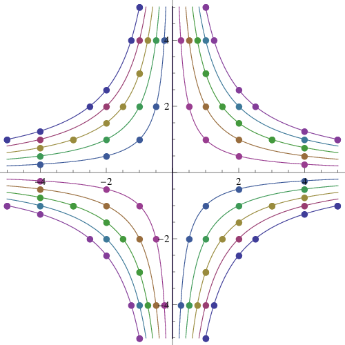
Figure 2 plots the value of the Blanchfield self-linking of elements in the rational Alexander module for the specific ribbon knot $\mathfrak{R}=9_{46}$ . Note that the Alexander module of $\mathfrak{R}$ is $\Delta_{\mathfrak{R}}(t)=2t^{2}-5t+2$ and its rational Alexander module is cyclic, generated by $\eta$ . Curves on the graph are given by $xy=c$ for $c\in\{\pm 1,\pm 2,\pm 3,\pm 4,\pm 5\}\subset\mathbb{Z}[1/2]$ . Each shaded point on the curve $xy=c$ is represented by an element of $\mathcal{A}^{\mathbb{Z}}(\mathfrak{R})$ whose Blanchfield self-linking, as an element of the rational Alexander module, is

c\cdot\mathcal{B}\ell(\eta,\eta)\in\frac{\mathbb{Q}(t)}{\mathbb{Q}[t,t^{-1}]}.

Furthermore, each of these elements in $\mathcal{A}^{\mathbb{Z}}(\mathfrak{R})$ is realized by an infecting curve, $\eta_{c}$ , in $S^{3}-\mathfrak{R}$ . By the proof of Corollary 3.3, there exists a knot $J$ such that the infection $\mathfrak{R}(\eta_{c},J)$ yields a distinct concordance class for each for each distinct $c\in\mathbb{Z}[1/2]$ . The verification of this graph will be given in Section 5

Proposition 3.5.

Let $\mathfrak{R}$ be a ribbon knot with Alexander polynomial $\Delta_{\mathfrak{R}}\neq 1$ . There exists a knot $J$ such that for any fixed infecting curve $\eta\subset S^{3}-\mathfrak{R}$ ,

\{[\gamma]|\mathfrak{R}(\gamma,J)\text{ is concordant to }\mathfrak{R}(\eta,J)\text{ for some }\gamma\in[\gamma]\}

is the subset of a quadric hypersurface in $\mathbb{Q}^{2g}$ .

Note that some restrictions on the infecting knot $J$ are necessary in the hypotheses of the reults presented. In particular, if $J$ is slice, $\mathfrak{R}(\eta,J)$ will always be concordant to $\mathfrak{R}$ .

Before beginning the technical details, we motivate our study with a few examples. Certainly, it seems that infection upon distinct infecting curves should describe distinct satellite operations and therefore produce nonconcordant knots. This is not always the case, however.

Example 1.1.

Take $\mathfrak{R}_{1}=9_{46}$ and let $\alpha,\beta$ be the infecting curves shown in Figure 3. Take $J$ to be any knot, and set $K_{1}\equiv\mathfrak{R}_{1}(\alpha,J)$ , $K_{2}\equiv\mathfrak{R}_{1}(\beta,J)$ . Notice that $\alpha$ and $\beta$ , as elements in $\mathcal{A}^{\mathbb{Z}}(\mathfrak{R}_{1})$ , have different orders and generate different submodules. However, both $\alpha$ and $\beta$ encircle ribbon bands of $\mathfrak{R}$ . If we cut along the band encircled by $\alpha$ in $K_{1}$ we obtain a two-component trivial link, shown in Figure 4, proving that $K_{1}$ is ribbon. Similary, $K_{2}$ is also ribbon and $K_{1}$ and $K_{2}$ are concordant in $\mathcal{C}$ .

In Example 1.1, $\alpha$ and $\beta$ generate different submodules and have different orders as elements of $\mathcal{A}^{\mathbb{Z}}(\mathfrak{R}_{1})$ . However, both submodules are isotropic with respect to the Blanchfield form, that is $\mathcal{B}\ell(\alpha,\alpha)=\mathcal{B}\ell(\beta,\beta)=0$ . This motivates our inquiry into how restrictions on the Blanchfield form could obstruct concordance between knots obtained by infecting $\mathfrak{R}$ using distinct infecting curves. These restrictions prove lucrative even if the infecting curves generate the same submodule and have the same order in the Alexander module, $\mathcal{A}(\mathfrak{R})$ . The following example illustrates that the question of which $\eta$ lead to distinct concordance classes is complicated even when $\mathcal{B}\ell(\eta,\eta)\neq 0$ .

Example 1.2.

Let $\mathfrak{R}_{2}=R_{1}\#R_{2}$ be the ribbon knot of Figure 5 formed by taking the connected sum of ribbon knots $R_{1},R_{2}$ . Here, the $1$ and $2$ inside the boxes indicate $1$ and $2$ negative full twists. Let $\eta_{1}$ and $\eta_{2}$ be the infecting curves shown in Figures 5a, 5b respectively. Again, take $J$ to be any knot, and set $K_{1}\equiv\mathfrak{R}_{2}(\eta_{1},J)$ , $K_{2}\equiv\mathfrak{R}_{2}(\eta_{2},J)$ . The Alexander module of $\mathfrak{R}_{2}$ is given by

\mathcal{A}^{\mathbb{Z}}(\mathfrak{R}_{2})=\mathcal{A}^{\mathbb{Z}}(R_{1})\oplus\mathcal{A}^{\mathbb{Z}}(R_{2})=\frac{\mathbb{Q}[t,t^{-1}]}{(1-2t)(2-1t)}\oplus\frac{\mathbb{Q}[t,t^{-1}]}{(2-3t)(3-2t)}

Notice that $\eta_{1}$ and $\eta_{2}$ generate different submodules of $\mathcal{A}^{\mathbb{Z}}(\mathfrak{R}_{2})$ , neither of which is isotropic. The orders of $[\eta_{1}],[\eta_{2}]$ are $(2-3t)(3-2t)$ and $(2-3t)(3-2t)(2-t)$ respectively. However, the Blanchfield form yields

\mathcal{B}\ell(\eta_{1},\eta_{1})=\frac{5(-1+t)^{2}}{6-13t+6t^{2}}=\mathcal{B}\ell(\eta_{2},\eta_{2}).

In fact, $K_{1}$ and $K_{2}$ are concordant! This is because the “extra band” encircled by $\eta_{2}$ is a ribbon band of $R_{1}$ . By cutting this band, we see that $\mathfrak{R}_{2}$ is concordant to $R_{2}$ , shown in Figure 6. Thus, in a similar process to that depicted in Figure 4, both $K_{1}$ and $K_{2}$ are concordant to $R_{2}(\eta,J)$ .

In Section 2, we provide the necessary terminology and preliminaries before formally introducing our main theorem in Section 3. Also in Section 3, we will also give a brief outline of its proof leaving some gaps. In 4 we go through the technical details to fill in these gaps, giving obstructions created by the Blanchfield form. Then, in Section 5, we give a complete study of distinct concordance classes, $K_{i}\equiv\mathfrak{R}(\eta_{i},J)$ , which may be produced by fixing the knot $J$ and setting $\mathfrak{R}\equiv 9_{46}$ as denoted in the Rolfsen knot tables [11]. This gives the necessary validation of Figure 2 as well as a detailed application of Corollary 3.3. Finally, in Section 6, we discuss an easier situation in which infecting curves have different orders in the Alexander module. In particular, this allows us to slightly ease the hypotheses on the infecting knot $J$ .

2. Background

2.1. The $n$ -solvable filtration of Cochran-Orr-Teichner

In order to establish our results, culminating in Corollary refcor:intense and Proposition 3.5, we rely on methods based on the $n$ -solvable filtration of the knot concordance group. Our methods ultimately prove a stronger result than knots $K_{1}\equiv\mathfrak{R}(\eta_{1},J)$ and $K_{2}\equiv\mathfrak{R}(\eta_{2},J)$ being nonconcordant, rather we show that ${K_{1}\#-K_{2}}$ is $2$ - but not $2.5$ -solvable according to this filtration. For any knot $K$ , we denote by $M_{K}$ the closed $3$ -manifold obtained by zero-surgery on $K$ in $S^{3}$ .

Definition 2.1.

[5, Definition 2.3] A knot $K$ is $n$ -solvable if there exists a spin $4$ -manifold $V$ with boundary $\partial V=M_{K}$ such that

(1)

Inclusion induces an isomorphism $H_{1}(M_{K};\mathbb{Z})\overset{\cong}{\longrightarrow}H_{1}(V;\mathbb{Z})$ .
(2)

There is a basis for $H_{2}(V;\mathbb{Z})$ , $\{L_{i},D_{j}|i,j=1,\dots,r\}$ , consisting of compact, connected, embedded surfaces with trivial normal bundles which are pairwise disjoint, except that for each $i$ , $L_{i}$ intersects $D_{i}$ transversely once with positive sign.
(3)

Inclusion induces $\pi_{1}(L_{i})\rightarrow\pi_{1}(V)^{(n)}$ , $\pi_{1}(D_{i})\rightarrow\pi_{1}(V)^{(n)}$ (where $G^{(n)}$ denotes the $n^{\text{th}}$ term of the derived series).

A knot is $n.5$ -solvable if, in addition,

(4)

$\pi_{1}(L_{i})\rightarrow\pi_{1}(V)^{(n+1)}$ .

$V$ is called the $n$ -solution (respectively the $n.5$ -solution) for $K$ . The subset of $\mathcal{C}$ consisting of all $n$ -solvable knots is denoted $\mathfrak{F}_{n}$ .

In addition, if we employ some arbitrary commutator series $*$ on $\pi_{1}(V)$ and property 3 (and 4) holds for $\pi_{1}(V)^{(n)}_{*}$ , we say that $K$ is $(n,*)$ -solvable (respectively $(n.5,*)$ -solvable). The set of $(n,*)$ -solvable knots is denoted by $\mathfrak{F}_{n}^{*}$ . These definitions induce a filtration on the concordance group of knots indexed by half integers, where $\mathfrak{F}_{n}\subset\mathfrak{F}_{n}^{*}$ for each $n\in\frac{1}{2}\mathbb{Z}$ [5, Proposition 2.5].

0\subset\bigcap\mathfrak{F}^{*}_{n}\subset\dots\subset\mathfrak{F}^{*}_{n.5}\subset\mathfrak{F}^{*}_{n}\subset\dots\subset\mathfrak{F}^{*}_{1}\subset\mathfrak{F}^{*}_{0.5}\subset\mathfrak{F}^{*}_{0}\subset\mathcal{C}

There has been much work using such filtrations (see [8, 5, 7, 6]). Knots which are $0$ -solvable are precisely those which have Arf-invariant zero, $1$ -solvable knots are algebraically slice, and any topologically slice knot is in $\mathfrak{F}_{n}$ for every $n\in\mathbb{Z}$ . Our results are based upon methods used in [5, 7, 6].

We suppose $\mathfrak{R}$ is a knot and $\eta_{1}$ , and $\eta_{2}$ are infecting curves in $S^{3}-\mathfrak{R}$ . Let $J$ and $L$ be two knots which may or may not be distinct. Then via infection, we form $K_{1}$ by removing a tubular neighborhood, $\nu(\eta_{1})$ , of $\eta_{1}$ in $M_{\mathfrak{R}}$ and replace it with a copy of $S^{3}-J$ along an identification of their common toric boundary. This process is done such that the longitude of $J$ is identified with the meridian of $\nu(\eta_{1})$ and the meridian of $J$ is identified with the reverse of the longitude of $\nu(\eta_{1})$ . We denote this operation by $K_{1}\equiv\mathfrak{R}(\eta_{1},J)$ . Form $K_{2}$ similarly by infecting $\mathfrak{R}$ along $\eta_{2}$ with $L$ . Note that infection is really just a specified satellite operation.

Theorem 2.2.

[5, Proposition 2.7] Suppose $J\in\mathfrak{F}^{*}_{n}$ , $\mathfrak{R}$ is ribbon, and $\eta\subset S^{3}-\mathfrak{R}$ is an infecting curve. If $[\eta]\in\pi_{1}(M_{\mathfrak{R}})_{*}^{(k)}$ , then $\mathfrak{R}(\eta,J)$ is $(n+k,*)$ -solvable.

Under certain conditions for the $\eta_{i}$ , $J$ , and $L$ , we show that $K_{1}$ and $K_{2}$ are not concordant. This is done by showing ${K_{1}\#-K_{2}}$ is not smoothly slice, as considered in the $(n,*)$ -solvable filtration. Both $J$ and $L$ will be $1$ -solvable, and by Theorem 2.2, both $K_{i}$ will lie in $\mathfrak{F}_{2}$ . We show that ${K_{1}\#-K_{2}}$ is not slice by showing that it is not $(2.5,\mathcal{S})$ -solvable where $\mathcal{S}$ is a commutator series defined in Definition 3.6.

2.2. Cheeger-Gromov constants, and the von Neumann $\rho$ -invariant

In the definition of an $n$ -solvable knot, we rely heavily on properties of the $n$ -solution $V$ . Therefore, we must look to invariants associated to this $4$ -manifold in order to obstruct $n.5$ -solvability.

Given a compact, orientable $4$ -manifold $X$ with boundary $\partial X=M_{K}$ , let $\Phi:\pi_{1}(X)\rightarrow\Lambda$ be a homomorphism where $\Lambda$ is a poly-torsion free abelian (PTFA) group [4, Definition 2.5],. If $\partial(X,\Phi)=(M_{K},\phi)$ , Cheeger and Gromov study the $\rho$ -invariant, denoted $\rho(M_{K},\phi)$ , associated to this coefficient system and show that it is equal to the “von Neumann signature defect” [3].

\rho(M_{K},\phi)=\sigma_{\Lambda}^{(2)}(X,\Phi)-\sigma(X)

In this equation, $\sigma_{\Lambda}^{(2)}(X,\Phi)$ is the $L^{(2)}$ signature of the equivariant intersection form defined on $H_{2}(X;\mathbb{Z}\Lambda)$ twisted by $\Phi$ and $\sigma(X)$ is the ordinary signature (See [8, Section 5]).

Proposition 2.3.

[7, Proposition 4.1]

(1)

If $\phi$ factors through $\phi^{\prime}:\pi_{1}(M_{K})\rightarrow\Lambda^{\prime}$ where $\Lambda^{\prime}$ is a subgroup of $\Lambda$ , then $\rho(M_{K},\phi^{\prime})=\rho(M_{K},\phi)$ .
(2)

If $\Phi$ is trivial on the restriction to $M_{K}\subset\partial X$ , then $\rho(M_{K},\phi)=0$ .
(3)

If $\phi:\pi_{1}(M_{K})\rightarrow\mathbb{Z}$ is the abelianization homomorphism, then $\rho(M_{K},\phi)$ is denoted by $\rho_{0}(K)$ and is equal to the integral of the Levine-Tristram signature function of $K$ .
(4)

The von Neumann signature defect satisfies Novikov additivity, i.e. if $X_{1}$ and $X_{2}$ intersect along a common boundary component and $\Phi_{i}$ is the restriction of $\Phi:X_{1}\cup X_{2}\rightarrow\Lambda$ to $X_{i}$ , then $\sigma_{\Lambda}^{(2)}(X_{1}\cup X_{2},\Phi)=\sigma_{\Lambda}^{(2)}(X_{1},\Phi_{1})+\sigma_{\Lambda}^{(2)}(X_{2},\Phi_{2})$ .
(5)

There is a positive real number $C_{K}$ called the Cheeger-Gromov constant of $M_{K}$ such that, for any $\phi:\pi_{1}(M_{K})\rightarrow\Lambda$ , $|\rho(M,\phi)|<C_{K}$ .
(6)

Let $*$ be an arbitrary commutator series and $K\in\mathfrak{F}_{n.5}^{*}$ via $X$ with $G=\pi_{1}(X)$ . If $\Phi:\pi_{1}(M)\rightarrow G/G_{*}^{(n+1)}=\Lambda$ , then

$\sigma_{\Lambda}^{(2)}(X,\Phi)-\sigma(X)=0=\rho(M,\Phi)$

Property 6 is integral to providing obstructions to solvability. If we assume $V$ is a $(2.5)$ -solution for ${K_{1}\#-K_{2}}$ , and $\Phi:\pi_{1}(V)\rightarrow\Lambda$ is trivial on $\pi_{1}(V)^{(3)}$ , then $\rho(M_{{K_{1}\#-K_{2}}},\phi)$ is trivial.

Using properties of the $\rho$ -invariants, we make the choice of $J$ explicit. First, let $J_{0}$ be an Arf-invariant zero knot. Take $R$ to be a ribbon knot with Alexander polynomial, $\Delta_{R}(t)\neq 1$ , and an infecting curve, $\beta$ in $S^{3}-R$ , which generates the rational Alexander module of $R$ . An example of such a choice is shown in Figure 7, where the $k$ in the box denotes $k$ negative full twists, and $\Delta_{R}(t)=\left(kt-(k+1)\right)\left((k+1)t-k)\right)$ . We will require that $J_{0}$ have $|\rho_{0}(J_{0})|>C_{R}+2C_{\mathfrak{R}}$ where $C_{R}$ and $C_{\mathfrak{R}}$ are the Cheeger-Gromov constants of $R$ and $\mathfrak{R}$ respectively (properties 3 and 5 of Proposition 2.3). By Theorem 2.2, $J\in\mathfrak{F}_{1}$ .

2.3. The Alexander Module and Blanchfield Form

For any knot $K$ with Alexander polynomial $\Delta_{K}(t)\neq 1$ , let $d$ be the leading coefficient of $\Delta_{K}(t)$ and $\mathcal{Q}=\mathbb{Z}[1/d]$ . The Alexander module of $K$ with $\mathcal{Q}$ -coefficients is defined by

\mathcal{A}^{\mathcal{Q}}(K)\equiv H_{1}(M_{K};\mathcal{Q}[t,t^{-1}])\cong\mathcal{A}^{\mathbb{Z}}(K)\otimes_{\mathbb{Z}}\mathcal{Q}.

As a $\mathcal{Q}$ -module, the Alexander module with $\mathcal{Q}$ coefficients is finitely generated and free, i.e. $\mathcal{A}^{\mathcal{Q}}(K)\cong\mathcal{Q}^{2g}$ where $g$ is the $3$ -genus of $K$ . Thus, any element $\gamma\in\mathcal{A}^{\mathcal{Q}}(K)$ may be described as a vector $(\gamma_{1},\dots,\gamma_{2g})\in\mathcal{Q}^{2g}$ .

Classically the Blanchfield form, $\mathcal{B}\ell^{\mathbb{Z}}_{K}(\cdot,\cdot)$ , is a sesquilinear form on the integral Alexander module of $K$ . This form has a generalization to the Alexander module with $\mathcal{Q}$ -coefficients.

Theorem 2.4.

[8, Theorem 2.13] If $\mathcal{Q}$ is any ring such that $\mathbb{Z}\subseteq\mathcal{Q}\subseteq\mathbb{Q}$ , then there is a nonsingular symmetric linking form

\mathcal{B}\ell^{\mathcal{Q}}_{K}:\mathcal{A}^{\mathcal{Q}}(K)\times\mathcal{Q}^{\mathcal{R}}(K)\rightarrow\mathbb{Q}(t)\mod\mathcal{Q}[t,t^{-1}].

We will employ the Blanchfield form with $\mathcal{Q}$ -coefficients for arbitrary $\mathbb{Z}\subseteq\mathcal{Q}\subseteq\mathbb{Q}$ and frequently alternate between coefficient systems. As we are primarily concerned with instances such that $\mathcal{B}\ell^{\mathcal{Q}}(x,x)\neq\mathcal{B}\ell^{\mathcal{Q}}(y,y)$ , the distinction is actually unnecessary for our purposes. Suppose $K$ is a knot with Alexander polynomial $\Delta_{K}(t)$ and $x$ and $y$ are infecting curves in $S^{3}-K$ . Also, let $x$ and $y$ denote the corresponding elements in $\mathcal{A}^{\mathbb{Z}}(K)$ . Then $x\otimes 1,y\otimes 1$ are the images of $x,y$ under the map

(1)

\mathcal{A}^{\mathbb{Z}}(K)\rightarrow\mathcal{A}^{\mathcal{Q}}(K)\cong\mathcal{A}^{\mathbb{Z}}(K)\otimes_{\mathbb{Z}}\mathcal{Q}

given by $z\mapsto z\otimes 1$ . Since $\mathcal{A}^{\mathbb{Z}}(K)$ has no $\mathbb{Z}$ -torsion, this map is injective. The following proposition, though easy to show, was not found in the literature. We prove it here for clarity.

Proposition 2.5.

For any ring $\mathcal{Q}$ such that $\mathbb{Z}\subseteq\mathcal{Q}\subseteq\mathbb{Q}$ ,

\mathcal{B}\ell^{\mathbb{Z}}(x,x)=\mathcal{B}\ell^{\mathbb{Z}}(y,y)\qquad\iff\qquad\mathcal{B}\ell^{\mathcal{Q}}(x\otimes 1,x\otimes 1)=\mathcal{B}\ell^{\mathcal{Q}}(y\otimes 1,y\otimes 1)

Proof.

The $\implies$ direction is obvious. We prove the $\Longleftarrow$ direction by contrapositive. Suppose $\mathcal{B}\ell^{\mathbb{Z}}(x,x)\neq\mathcal{B}\ell^{\mathbb{Z}}(y,y)$ . Then

\mathcal{B}\ell^{\mathbb{Z}}(x,x)-\mathcal{B}\ell^{\mathbb{Z}}(y,y)=\frac{p(t)}{\delta_{K}(t)}\in\mathbb{Q}(t)\mod\mathbb{Z}[t,t^{-1}]

where $(p(t),\delta_{K}(t))=1$ and $\delta_{K}(t)$ divides $\Delta_{K}(t)$ . Notice that the field of fractions of both $\mathbb{Z}[t,t^{-1}]$ and $\mathcal{Q}[t,t^{-1}]$ is $\mathbb{Q}(t)$ and the ring monomorphism $\mathbb{Z}\hookrightarrow\mathcal{Q}$ induces the following $\mathbb{Z}[t,t^{-1}]$ -module homomorphisms.

\begin{array}[]{rl}h:&\mathbb{Q}(t)\hookrightarrow\mathbb{Q}(t)\\ \overline{h}:&\mathbb{Q}(t)/\mathbb{Z}[t,t^{-1}]\rightarrow\mathbb{Q}(t)/\mathcal{Q}[t,t^{-1}]\\ h_{\ast}:&\mathcal{A}^{\mathbb{Z}}(K)\rightarrow\mathcal{A}^{\mathcal{Q}}(K)\cong\mathcal{A}^{\mathbb{Z}}(K)\otimes_{\mathbb{Z}}\mathcal{Q}\end{array}

The first map is the identity and the third is equivalent to the map of Equation 1. However, given any element $z\in\mathcal{A}^{\mathbb{Z}}(K)$ , we have

\mathcal{B}\ell^{\mathcal{Q}}(z\otimes 1,z\otimes 1)=\overline{h}(\mathcal{B}\ell^{\mathbb{Z}}(z,z))

[9, Theorem 4.7]. If $\mathcal{B}\ell^{\mathcal{Q}}(x\otimes 1,x\otimes 1)-\mathcal{B}\ell^{\mathcal{Q}}(y\otimes 1,y\otimes 1)=0$ , this implies

\overline{h}\left(\frac{p(t)}{\delta_{K}(t)}\right)=0.

The map $\overline{h}$ is given by modding out by the subring $\mathcal{Q}[t,t^{-1}]/\mathbb{Z}[t,t^{-1}]\subset\mathbb{Q}(t)/\mathbb{Z}[t,t^{-1}]$ . This means $\frac{p(t)}{\delta_{K}(t)}$ reduces to a polynomial $F(t)\in\mathcal{Q}[t,t^{-1}]$ . After multiplying through by some constant $q\in\mathbb{Z}$ which is a unit in $\mathcal{Q}$ , we obtain the following equation in $\mathbb{Z}[t,t^{-1}]$ :

q\cdot p(t)=f(t)\delta_{K}(t),

where $q\cdot F(t)=f(t)\in\mathbb{Z}[t,t^{-1}]$ . Since $\delta_{K}(1)=\pm 1$ , regarding $q$ as a constant polynomial in $\mathbb{Z}[t,t^{-1}]$ , $(q,\delta_{K}(t))=1$ , so $q$ divides $f(t)$ . This means

\frac{p(t)}{\delta_{K}(t)}=\frac{f(t)}{q}\in\mathbb{Z}[t,t^{-1}],

and so $\mathcal{B}\ell^{\mathbb{Z}}(x,x)-\mathcal{B}\ell^{\mathbb{Z}}(y,y)=0$ in $\mathbb{Q}(t)/\mathbb{Z}[t,t^{-1}]$ , a contradiction. ∎

Because of Proposition 2.5, we are free to suppress the distinction between the integral and rational Blanchfield forms in comparing the Blanchfield self-linking of two infecting curves. We will frequently pass between the two and, by an abuse of notation, allow $\mathcal{B}\ell(x,x)$ to identify both $\mathcal{B}\ell^{\mathbb{Z}}(x,x)$ and $\mathcal{B}\ell^{\mathcal{Q}}(x\otimes 1,x\otimes 1)$ where understood.

Recall that $\eta_{1}$ and $\eta_{2}$ are infecting curves for $\mathfrak{R}$ , and $J$ is a $1$ -solvable knot defined by $J=R(\beta,J_{0})$ where $|\rho_{0}(J_{0})|>C_{R}+2C_{\mathfrak{R}}$ . Then, require $L$ to be any $1$ -solvable knot with Alexander polynomial $\Delta_{L}(t)$ satisfying one of the two following conditions:

(1)

$\Delta_{R}$ and $\Delta_{L}$ are strongly coprime, i.e. $\Delta_{R}(t^{n}),\Delta_{L}(t^{m})$ are relatively prime for every $n,m\in\mathbb{Z}$ .
(2)

$\Delta_{R}(t^{m})$ and $\Delta_{L}(t^{n})$ have no common roots unless $n=\pm m$ .

Certainly (1) implies (2). If (1) holds, $K_{1}\equiv\mathfrak{R}(\eta_{1},J)$ and $K_{2}\equiv\mathfrak{R}(\eta_{2},L)$ are distinct (and even linearly independent) in $\mathcal{C}$ by a generalization of Cochran-Harvey-Leidy [5]. If 2, a secondary restriction will be given by the Blanchfield self-linking of the infecting curves $\eta_{1},\eta_{2}$ . In particular, we need only require that $\mathcal{B}\ell(\eta_{1},\eta_{1})\neq\mathcal{B}\ell(\eta_{2},\eta_{2})$ .

3. The Main Theorems

Theorem 3.1.

If $R$ and $\mathfrak{R}$ are ribbon knots, let $J_{0}$ be an Arf-invariant zero knot such that $|\rho_{0}(J_{0})|>C_{R}+2C_{\mathfrak{R}}$ . Suppose $J\equiv R(\beta,J_{0})$ where $\beta$ generates the rational Alexander module of $R$ . Then form $K_{1}\equiv\mathfrak{R}(\eta_{1},J)$ where $\mathcal{B}\ell(\eta_{1},\eta_{1})\neq 0$ and $K_{2}\equiv\mathfrak{R}(\eta_{2},L)$ . If $L$ is any $1$ -solvable knot such that

(1)

$\Delta_{L}(t)$ and $\Delta_{R}(t)$ are strongly coprime, or
(2)

$\Delta_{L}(t^{m})$ and $\Delta_{R}(t^{n})$ share a common root only when $n=\pm m$ and $\mathcal{B}\ell(\eta_{1},\eta_{1})\neq\mathcal{B}\ell(\eta_{2},\eta_{2})$ ,

Then $K_{1}$ and $K_{2}$ are distinct in $\mathcal{C}$ .

Before describing an outline of this proof, we introduce the following corollaries which illustrate the impact of Theorem 3.1.

Corollary 3.2.

Suppose $J\equiv R(\beta,J_{0})$ where $J_{0}$ is an Arf-invariant zero knot, $R$ is the ribbon knot from Figure 7 with $\beta$ as shown. Let $K_{1}\equiv\mathfrak{R}(\eta_{1},J)$ and $K_{2}\equiv\mathfrak{R}(\eta_{2},J)$ . If $|\rho_{0}(J_{0})|>C_{R}+2C_{\mathfrak{R}}$ and $\mathcal{B}\ell_{\mathfrak{R}}(\eta_{1},\eta_{1})\neq\mathcal{B}\ell_{\mathfrak{R}}(\eta_{2},\eta_{2})$ then $K_{1}$ and $K_{2}$ are not concordant.

Proof that Theorem 3.1 implies Corollary 3.2.

We assume without loss of generality $\mathcal{B}\ell(\eta_{1},\eta_{1})\neq 0$ . Since $\Delta_{R}(t)=\Delta_{J}(t)=(kt-(k+1))((k+1)t-k)$ has roots $\{\frac{k}{k+1},\frac{k+1}{k}\}$ , $\Delta_{R}(t^{m})$ and $\Delta_{R}(t^{n})$ share no common roots unless $n=\pm m$ . The result follows from Theorem 3.1. ∎

The above stress the distinction between any two infecting curves. We next generalize these results to produce infinitely many distinct concordance classes.

Corollary 3.3.

Suppose $\mathfrak{R}$ is any knot with $\Delta_{\mathfrak{R}}\neq 1$ . Then there exists a (countably infinite) set of curves $\{\eta_{i}\}$ in $S^{3}-\mathfrak{R}$ which are unknotted in $S^{3}$ and have linking number $0$ with $\mathfrak{R}$ , and also a knot $J$ such that each $K_{i}\equiv\mathfrak{R}(\eta_{i},J)$ generates a distinct concordance class in $\mathcal{C}$ .

Proof.

In order to employ Corollary 3.2, we must ensure the existence of an infinite family of curves $\eta_{i}$ which have distinct Blanchfield self-linking, i.e. $\mathcal{B}\ell(\eta_{i},\eta_{i})=\mathcal{B}\ell(\eta_{j},\eta_{j})$ only when $i=j$ . Since $\mathfrak{R}$ has nontrivial Alexander polynomial and the Blanchfield form on $\mathcal{A}^{\mathbb{Z}}(\mathfrak{R})$ is nonsingular, there must exist some curve $\eta\subset S^{3}-J$ such that $\mathcal{B}\ell(\eta,\eta)\neq 0$ . We use the following proposition.

Proposition 3.4.

Suppose $\eta\subset S^{3}-\mathfrak{R}$ is an unknotted curve in $S^{3}$ with $lk(\eta,\mathfrak{R})=0$ and $\mathcal{B}\ell(\eta,\eta)\neq 0$ . For each $i\in\mathbb{Z}_{\geq 0}$ , set $\eta_{i}=i\eta\in\mathcal{A}^{\mathbb{Z}}(\mathfrak{R})$ . Then $\mathcal{B}\ell(\eta_{i},\eta_{i})=\mathcal{B}\ell(\eta_{j},\eta_{j})$ only when $i=j$ , and each $\eta_{i}$ is represented by an unknotted curve in $S^{3}-\mathfrak{R}$ .

Proof.

Suppose $\mathcal{B}\ell(\eta,\eta)=\frac{p(t)}{\delta_{\mathfrak{R}}(t)}\notin\mathbb{Z}[t,t^{-1}]$ such that $(p(t),\delta_{\mathfrak{R}}(t))=1$ and $\delta_{\mathfrak{R}}(t)$ divides $\Delta_{\mathfrak{R}}(t)$ . Then we have

\mathcal{B}\ell(\eta_{i},\eta_{i})=\mathcal{B}\ell(i\eta,i\eta)=i^{2}\mathcal{B}\ell(\eta,\eta)=i^{2}\frac{p(t)}{\delta_{\mathfrak{R}}(t)}

If $\mathcal{B}\ell(\eta_{i},\eta_{i})=\mathcal{B}\ell(\eta_{j},\eta_{j})$ , this implies $(i^{2}-j^{2})\mathcal{B}\ell(\eta,\eta)=f(t)\in\mathbb{Z}[t,t^{-1}]$ . We have the following equation

(i^{2}-j^{2})p(t)=f(t)\delta_{\mathfrak{R}}(t)

where, since $\frac{p(t)}{\delta_{\mathfrak{R}}(t)}\neq 0$ , we can assume that $i^{2}-j^{2}$ does not divide $f(t)$ over $\mathbb{Z}[t,t^{-1}]$ . Since $\delta_{\mathfrak{R}}(q)=\pm 1$ , $i^{2}-j^{2}\in\{0,\pm 1\}$ . If $i^{2}-j^{2}=\pm 1$ , this contradicts $\mathcal{B}\ell(\eta,\eta)\neq 0$ . As $i,j\geq 0$ , $i^{2}-j^{2}$ is zero only when $i=j$ . We must next show that each $\eta_{i}$ is unknotted in $S^{3}$ . But notice that the element $i\eta\in\mathcal{A}^{\mathbb{Z}}(\mathfrak{R})$ is realized by the $(i,1)$ -cable of $\eta$ . This completes the proof. ∎

By taking $J$ to be the knot given in the statement of Corollary 3.2, we obtain a family of pairwise distinct concordance classes $\{K_{i}\equiv\mathfrak{R}(\eta_{i},J)\}$ for $i\geq 0$ . ∎

The following corollary illustrates how uncommon it is for two infecting curves, $\eta$ and $\gamma$ in $S^{3}-\mathfrak{R}$ to yield concordant knots. By viewing them as elements of $\mathcal{A}^{\mathbb{Q}}(K)\cong\mathbb{Q}^{2g}$ , we get an approximate answer to this question by seeing that the set of infecting curves $\gamma$ which yield knots concordant to $K=\mathfrak{R}(\eta,J)$ must lie on a quadratic hypersurface in $\mathbb{Q}^{2g}$ .

Proposition 3.5.

Let $\mathfrak{R}$ be a ribbon knot with Alexander polynomial $\Delta_{\mathfrak{R}}\neq 1$ and $J\equiv R(\beta,J_{0})$ as above. Fix some infecting curve $\eta\subset S^{3}-\mathfrak{R}$ and let $K\equiv\mathfrak{R}(\eta,J)$ . Then,

\{[\gamma]|\mathcal{B}\ell(\gamma,\gamma)=\mathcal{B}\ell(\eta,\eta)\}

is the subset of a quadric hypersurface in $\mathbb{Q}^{2g}$ , and thus $\{[\gamma]|K^{\prime}=\mathfrak{R}(\gamma,J_{0})\text{ is not concordant to }K\}$ is dense as a subset of $\mathbb{Q}^{2g}$ .

Proof.

Following work of Trotter [15, 14], let $z=(1-t)^{-1}$ and note that $\mathbb{Q}(t)=\mathbb{Q}(z)$ . Furthermore, since $z$ gives an automorphism of $\mathcal{A}^{\mathbb{Z}}(K)$ , enlarging coefficients from $\mathbb{Z}[t,t^{-1}]$ to $\mathbb{Z}[t,t^{-1},z]$ has no effect on the module structure. Consider the map

\frac{\mathbb{Q}(t)}{\mathbb{Z}[t,t^{-1}]}\xrightarrow{j}\frac{\mathbb{Q}(t)}{\mathbb{Z}[t,t^{-1},z]}

given by inclusion. The form given by $\widehat{\mathcal{B}\ell}(x,y)=j(\mathcal{B}\ell(x,y))$ is a nonsingular sesquilinear form and $j$ maps the image of $\mathcal{B}\ell(\cdot,\cdot)$ one-to-one onto the image of $\widehat{\mathcal{B}\ell}(\cdot,\cdot)$ [15].

Using a partial fraction decomposition, any element in $\mathbb{Q}(t)$ may be written uniquely as the sum of a polynomial and proper fractions where the numerator has lower degree than the denominator. Thus, $\mathbb{Q}(t)$ splits over $\mathbb{Q}$ as the direct sum of $\mathbb{Q}[t.t^{-1},z]$ and a subspace $P$ where $P$ consists of $0$ and proper fractions with denominator coprime to $t$ and $1-t$ . Then we have a $\mathbb{Q}$ -linear map $\chi:\mathbb{Q}(t)\rightarrow\mathbb{Q}$ defined by

\chi(f)=\left\{\begin{array}[]{ll}f^{\prime}(1)&f\in P\\ 0&f\in\mathbb{Q}[t,t^{-1},z]\end{array}\right.

Since $\chi$ is $0$ on $\mathbb{Q}[t,t^{-1},z]$ , it is well defined on $\mathbb{Q}(z)\mod\mathbb{Q}[t,t^{-1},z]$ and thus on the image of $\widehat{\mathcal{B}\ell}$ . Note that the value of $\widehat{\mathcal{B}\ell}(x,y)$ is uniquely determined by the value of $\chi(\lambda\widehat{\mathcal{B}\ell}(x,y))$ for all $\lambda\in\mathbb{Z}[t,t^{-1},z]$ , and furthermore, $\chi$ satisfies

\chi(\overline{f})=\chi(f)\qquad\chi((t-1)f)=f(1)

for any $f\in P$ [14, Section 2]. Since $\mathcal{B}\ell(x,y)=\overline{\mathcal{B}\ell(y,x)}$ for any $x,y\in\mathcal{A}^{\mathbb{Z}}(K)$ , $\chi(\widehat{\mathcal{B}\ell}(\gamma,\gamma))=0$ for all $\gamma$ . This is also seen by noting that, by definition, $\mathcal{B}\ell$ is given by

\mathcal{B}\ell(x,y)=\overline{y}(1-t)\left(tV-V^{\intercal}\right)^{-1}x.

Since $\mathcal{B}\ell$ is nonsingular, there must exist some $\lambda_{0}\in\mathbb{Z}[t,t^{-1},z]$ such that $\chi(\lambda_{0}\mathcal{B}\ell(x,x))$ is nonzero for some $x\in\mathcal{A}^{Z}(K)$ . For $\gamma\in S^{3}-K$ , define $\widehat{\chi}:\mathcal{A}^{\mathbb{Q}}(K)\cong\mathbb{Q}^{2g}\rightarrow\mathbb{Q}$ by

\displaystyle\widehat{\chi}(\gamma)

\displaystyle\equiv\chi((\lambda_{0}\widehat{\mathcal{B}\ell}(\gamma,\gamma)).

Suppose $\widehat{\chi}(\eta)=c\in\mathbb{Q}$ . Then $\widehat{\chi}(x_{1},\dots,x_{2g})=c$ is a rational equation in $2g$ variables and the left-hand side is a homogeneous polynomial of degree $2$ . That is,

	$\displaystyle\widehat{\chi}(x_{1},\dots,x_{2g})=$	$\displaystyle\sum_{i,j}\chi\left(\lambda_{0}\mathcal{B}\ell(x_{i},x_{j})\right)$
	$\displaystyle=$	$\displaystyle\sum_{i,j}x_{i},x_{j}\chi\left(\lambda_{0}\mathcal{B}\ell(e_{i},e_{j})\right)$
	$\displaystyle=$	$\displaystyle\sum_{i,j}a_{i,j}x_{i}x_{j}=c$

where $a_{i,j}=\chi\left(\lambda_{0}\mathcal{B}\ell(e_{i},e_{j})\right)$ and $\{e_{i}\}$ is a basis for $\mathcal{A}^{\mathbb{Q}}(K)\cong\mathbb{Q}^{2g}$ . Since $\mathcal{B}\ell$ is nonsingular, not all $a_{i,j}=0$ . By Theorem 3.1, the set of infecting curves $\gamma\subset S^{3}-\mathfrak{R}$ such that $K^{\prime}=\mathfrak{R}(\gamma,J)$ is concordant to $K=\mathfrak{R}(\eta,J)$ must be ones such that $\mathcal{B}\ell(\gamma,\gamma)=\mathcal{B}\ell(\eta,\eta)$ . Therefore $\gamma=(\gamma_{1},\dots,\gamma_{2g})$ must be a solution to $\widehat{\chi}(x_{1},\dots,x_{2g})=c$ .

Consider the polynomial $F(x_{1},\dots,x_{2g})=\widehat{\chi}(x_{1},\dots,x_{2g})-c=0$ . If $c\neq 0$ , this polynomial is clearly nonconstant. Otherwise, given the choice of $\lambda_{0}$ and that $\mathcal{B}\ell$ is nonsingular there must exist some element $\gamma\in\mathcal{A}^{\mathbb{Z}}$ such that $\widehat{\chi}(\gamma)\neq 0$ and hence $F(\gamma)\neq 0$ and $F$ is a nonconstant polynomial. The zero locus of $\widehat{\chi}(x_{1},\dots,x_{2g})-c$ is a quadric hypersurface in $\mathbb{Q}^{2g}$ whose compliment is dense. ∎

In the proof Proposition 3.5, we distinguish infecting curves by evaluating Trotter’s trace function $\chi$ on $\lambda_{0}\widehat{\mathcal{B}\ell}(\gamma,\gamma)$ for one particular value $\lambda_{0}\in\mathbb{Q}[t,t^{-1},z]$ . Since $\widehat{\mathcal{B}\ell}(\gamma,\gamma)$ is uniquely determined by the value of $\chi(\lambda\widehat{\mathcal{B}\ell}(\gamma,\gamma))$ for all $\lambda\in\mathbb{Q}[t,t^{-1},z]$ , one could attempt to distinguish the infecting curves $\gamma$ and $\eta$ by using multiple values of $\lambda$ when $\chi(\lambda_{0}\widehat{\mathcal{B}}\ell(\gamma,\gamma))=\chi(\lambda_{0}\widehat{\mathcal{B}}\ell(\eta,\eta))$ .

We now proceed to the proof of Theorem 3.1.

Proof of Theorem 3.1.

We will show the stronger fact that ${K_{1}\#-K_{2}}$ is not $2.5$ -solvable. The proof is by contradiction. ${K_{1}\#-K_{2}}$ is $2$ -solvable by [5, Proposition 2.7], and suppose it is $2.5$ -solvable via $V$ . We construct a tower of cobordisms for $M_{{K_{1}\#-K_{2}}}$ . Note that from the infection operation arises a natural cobordism between zero surgeries on the knots involved. Given that $K_{1}\equiv\mathfrak{R}(\eta_{1},J)$ , denote by $F_{1}$ the cobordism obtained by first taking the disjoint union of $M_{\mathfrak{R}}\times[0,1]$ and $M_{J}\times[0,1]$ . Then identify a neighborhood of $\eta_{1}\times\{1\}$ , denoted by $\nu(\eta_{1})$ , in $M_{\mathfrak{R}}\times\{1\}$ with $\nu(J)$ , a neighborhood of $J\times\{1\}$ in $M_{J}\times\{1\}$ given by $\left(M_{J}\setminus(S^{3}-J)\right)\times\{1\}$ as shown in Figure 8. This identification is done such that the longitude of $\nu(J)$ is identified with the meridian of $\nu(\eta_{1})$ and the meridian of $\nu(J)$ is identified with the reverse of the longitude of $\nu(\eta_{1})$ . That is,

F_{1}\equiv\frac{(M_{\mathfrak{R}}\times[0,1])\cup(M_{J}\times[0,1])}{\nu(\eta_{1})\sim\nu(J)}

The boundary of $F_{1}$ is then given by $\partial F_{1}=M_{\mathfrak{R}}\sqcup M_{J}\sqcup\overline{M_{K_{1}}}$ , where by $\overline{X}$ , we mean the manifold $X$ with opposite orientation. Similarly, we let $F_{2}$ denote a cobordism given by the infections $K_{2}=\mathfrak{R}(\eta_{2},L)$ . The infection $J\equiv R(\beta,J_{0})$ will yield a cobordism denoted $G$ . Since connected sum ${K_{1}\#-K_{2}}$ may also be viewed as the infection of $K_{1}$ by $-K_{2}$ along a meridian, form a cobordism $E$ between zero surgeries on $K_{1}$ , $-K_{2}$ , and ${K_{1}\#-K_{2}}$ in a similar manner. Define $W^{\prime}$ to be the union of $V$ and $E$ along their common boundary. Similarly, $W$ is the union $W^{\prime}\cup F_{1}\cup\overline{F_{2}}$ . Then, let $Z$ be the manifold obtained by joining the cobordisms $G$ to $W$ along $M_{J}$ . The boundary of $Z$ is given by $\partial Z=M_{\mathfrak{R}}\sqcup M_{R}\sqcup M_{J_{0}}\sqcup\overline{M_{\mathfrak{R}}}\sqcup\overline{M_{L}}$ . In overview,

	$\displaystyle\partial V$	$\displaystyle=M_{{K_{1}\#-K_{2}}}$
	$\displaystyle\partial E$	$\displaystyle=M_{K_{1}}\sqcup M_{K_{2}}\sqcup\overline{M_{{K_{1}\#-K_{2}}}}$
	$\displaystyle\partial F_{1}$	$\displaystyle=M_{J}\sqcup M_{\mathfrak{R}}\sqcup\overline{M_{K_{1}}}$
	$\displaystyle\partial F_{2}$	$\displaystyle=M_{L}\sqcup M_{\mathfrak{R}}\sqcup\overline{M_{K_{2}}}$
	$\displaystyle\partial G$	$\displaystyle=M_{J_{0}}\sqcup M_{R}\sqcup\overline{M_{J}}$

	$\displaystyle W^{\prime}$	$\displaystyle=V\cup_{M_{{K_{1}\#-K_{2}}}}E$
	$\displaystyle W$	$\displaystyle=W^{\prime}\cup_{M_{K_{1}}}F_{1}\cup_{\overline{M_{K_{2}}}}\overline{F_{2}}$
	$\displaystyle Z$	$\displaystyle=W\cup_{M_{J}}G.$

Unfortunately, the derived series itself will not be useful in finding an obstruction to the $2.5$ -solvablity of ${K_{1}\#-K_{2}}$ . Instead, we define a partial commutator series, $\mathcal{S}$ , which will be slightly larger than the rational derived series so that

\pi_{1}(Z)^{(3)}\subset\pi_{1}(Z)_{\mathcal{S}}^{(3)}.

Notice in Definition 3.6, $\mathcal{S}$ will be equivalent to the rational derived series on its first two terms.

Definition 3.6.

Let $G$ be a group with $G/G^{(1)}=\langle\mu\rangle\cong\mathbb{Z}$ , then the derived series localized at $\mathcal{S}$ is defined recursively by

\begin{split}G^{(0)}_{\mathcal{S}}&\equiv G\\ G^{(1)}_{\mathcal{S}}=G_{r}^{(1)}&\equiv\ker\left(G\rightarrow\frac{G}{[G,G]}\otimes_{\mathbb{Z}}\mathbb{Q}\right)\\ G^{(2)}_{\mathcal{S}}=G_{r}^{(2)}&\equiv\ker\left(G_{\mathcal{S}}^{(1)}\rightarrow\frac{G_{\mathcal{S}}^{(1)}}{[G_{\mathcal{S}}^{(1)},G_{\mathcal{S}}^{(1)}]}\otimes_{\mathbb{Z}[G/G_{\mathcal{S}}^{(1)}]}\mathbb{Q}[G/G_{\mathcal{S}}^{(1)}]\right)\\ G_{\mathcal{S}}^{(3)}&\equiv\ker\left(G_{\mathcal{S}}^{(2)}\rightarrow\frac{G_{\mathcal{S}}^{(2)}}{[G_{\mathcal{S}}^{(2)},G_{\mathcal{S}}^{(2)}]}\otimes_{\mathbb{Z}[G/G_{\mathcal{S}}^{(2)}]}\mathbb{Q}[G/G_{\mathcal{S}}^{(2)}]S^{-1}\right).\end{split}

The right divisor set $S~\subset~\mathbb{Q}[G_{\mathcal{S}}^{(1)}/G^{(2)}_{\mathcal{S}}]\subset\mathbb{Q}[G/G^{(2)}_{\mathcal{S}}]$ is the multiplicative set generated by $\{\Delta_{L}(\mu^{i}\eta_{2}^{\prime}\mu^{-i})|i\in\mathbb{Z}\}$ . Here, ${\eta_{2}}^{\prime}$ denotes the image of $\eta_{2}$ in $M_{-\mathfrak{R}}\subset M_{{\mathfrak{R}\#-\mathfrak{R}}}$ and is considered as an element of $\pi_{1}(W)$ by inclusion. $S$ is by definition a multiplicatively closed set with unity, and $0$ is not an element of $\mathcal{S}$ . Since $\mathbb{Q}[G^{(1)}/G_{\mathcal{S}}^{(2)}]$ is abelian, this verifies $S$ is a right divisor set. Furthermore, let $\gamma\in G/G_{\mathcal{S}}^{(2)}$ . If $q(a)\in S$ , then $\gamma q(a)\gamma^{-1}=q(\gamma a\gamma^{-1})\in S$ . Therefore, $\mu^{i}\eta_{2}^{\prime}\mu^{-i}$ is invariant under conjugation by $G/G_{\mathcal{S}}^{(2)}$ , and we see that $S$ is invariant under conjugation by $\mathbb{Q}[G/G_{\mathcal{S}}^{(2)}]$ .

Consider the coefficient system on $W$ given by the projection

\Phi:\pi_{1}(Z)\rightarrow\pi_{1}(Z)/\pi_{1}(Z)^{(3)}\rightarrow\pi_{1}(Z)/\pi_{1}(Z)^{(3)}_{\mathcal{S}}\equiv\Lambda

Because of property (4) of Proposition 2.3 (and after suppressing notation by $\sigma_{\Lambda}^{(2)}\equiv\sigma^{(2)}\text{ and }\Phi|_{X}\equiv\Phi$ where understood), we have

(2)

\begin{split}\sigma^{(2)}(Z,\Phi)-\sigma(Z)=&\left(\sigma^{(2)}(V,\Phi)-\sigma(V)\right)+\left(\sigma^{(2)}(E,\Phi)-\sigma(E)\right)+\left(\sigma^{(2)}(F_{1},\Phi)-\sigma(F_{1})\right)\\ &+\left(\sigma^{(2)}(\overline{F_{2}},\Phi)-\sigma(\overline{F_{2}})\right)+\left(\sigma^{(2)}(G,\Phi)-\sigma(G)\right)\end{split}

By assumption, $V$ is a $2.5$ -solution. Property (6) of Proposition 2.3 yields $\sigma^{(2)}(V,\Phi)-\sigma(V)=0$ . For $E,F_{1},F_{2},$ and $G$ , all of the (integral and twisted) second homology comes from the boundary [6, Lemma 2.4], and therefore

\sigma^{(2)}(E,\Phi)-\sigma(E)=\sigma^{(2)}(F_{1},\Phi)-\sigma(F_{1})=\sigma^{(2)}(F_{2},\Phi)-\sigma(F_{2})=\sigma^{(2)}(G,\Phi)-\sigma(G)=0.

However, $\sigma^{(2)}(Z,\Phi)-\sigma(Z)=\rho(\partial Z,\Phi|_{\partial})$ , and

0=\rho(\partial Z,\Phi)=\rho(M_{J_{0}},\Phi)+\rho(\overline{M_{L}},\Phi)+\rho(M_{\mathfrak{R}},\Phi)+\rho(\overline{M_{\mathfrak{R}}},\Phi)+\rho(M_{R},\Phi).

We employ the following lemmas, to be proven in Section 4.

Lemma 4.2 The restriction of $\Phi$ to $\pi_{1}(M_{J_{0}})$ factors non-trivially through $\mathbb{Z}$ .

Lemma 4.4 The restriction of $\Phi$ to $\pi_{1}(M_{L})$ also factors through $\mathbb{Z}$ and yields $\rho(M_{L},\Phi)=0.$

After proving Lemma 4.2 and using properties (1) and (3) of Proposition 2.3, we will have $\rho(M_{J_{0}},\Phi)=\rho_{0}(J_{0})$ . Secondly, by Lemma 4.4 and property (2) of Proposition 2.3, $\rho(\overline{M_{L}},\Phi)=-\rho(M_{L},\Phi)=0$ . This yields the following equation.

\rho_{0}(J_{0})=-\rho(M_{\mathfrak{R}},\Phi)-\rho(M_{-\mathfrak{R}},\Phi)-\rho(M_{R},\Phi).

This is a contradiction since, by hypothesis,

|\rho_{0}(J_{0})|>C_{R}+2C_{\mathfrak{R}}\geq\rho(M_{\mathfrak{R}},\Phi)+\rho(M_{-\mathfrak{R}},\Phi)+\rho(M_{R},\Phi)

This completes the proof modulo the proofs of Lemmas 4.2 and 4.4 ∎

4. Blanchfield Form Restrictions

In this section, we prove the Lemmas needed for the completion of Theorem 3.1. We continue to use notation which was defined in Sections 2 and 3. Before proving Lemma 4.2, we must first show that the infecting curve $\eta_{1}$ represents a nontrivial element of $\pi_{1}(W)^{(1)}/\pi_{1}(W)_{\mathcal{S}}^{(2)}$ by inclusion. Note that $\pi_{1}(M_{J_{0}})$ is normally generated by the meridian $\mu_{0}$ which is isotopic in $Z$ to the $\beta\in\pi_{1}(M_{R})^{(1)}$ . Similarly, the meridian of $M_{R}$ is identified with $\eta_{1}$ and inclusion induces

\eta_{1}\in\pi_{1}(M_{\mathfrak{R}})^{(1)}\subset\pi_{1}(W)^{(1)}\subset\pi_{1}(Z)^{(1)}

which implies that $\mu_{0}\sim\beta$ is in $\pi_{1}(Z)^{(2)}$ . If $\eta_{1}\in\pi_{1}(Z)^{(2)}$ , then $\pi_{1}(M_{J_{0}})$ is mapped to a subset of $\pi(Z)^{(3)}$ and the restriction of $\Phi$ to $\pi_{1}(M_{J_{0}})$ is trivial.

Continue to let $\eta_{2}^{\prime}\subset M_{{\mathfrak{R}\#-\mathfrak{R}}}$ denote the image of $\eta_{2}$ after reversing the orientation of $M_{\mathfrak{R}}$ and taking the connected sum to form $M_{{\mathfrak{R}\#-\mathfrak{R}}}$ . By an abuse of notation, $\eta_{1}$ and $\eta_{2}^{\prime}$ also represent the corresponding elements in the Alexander module and $\pi_{1}$ . Let $\mathcal{A}(X)$ denote the Alexander module of the space $X$ with rational coefficients. The following proofs closely follow the methodology of [7, Lemmas 7.6, 7.6]

Lemma 4.1.

The infecting curve $\eta_{1}$ represents a nontrivial element of $A\equiv\pi_{1}(W)^{(1)}/\pi_{1}(W)^{(2)}_{\mathcal{S}}$

Proof.

Consider the following commutative diagram of Alexander modules.

(3)

\begin{diagram}

The validity of this diagram is supported by the fact that $\mathcal{A}^{\mathbb{Z}}({K_{1}\#-K_{2}})\cong\mathcal{A}^{\mathbb{Z}}({\mathfrak{R}\#-\mathfrak{R}})$ . The horizontal maps are induced by inclusion. Since $\mathcal{A}^{\mathbb{Z}}({\mathfrak{R}\#-\mathfrak{R}})$ is $\mathbb{Z}$ torsion free, $i_{1}$ is injective. By Definition 3.6, $\pi_{1}(W)^{(2)}_{\mathcal{S}}\equiv\pi_{1}(W)^{(2)}_{r}$ , and therefore $i_{6}:\pi_{1}(W)^{(1)}/\pi_{1}(W)^{(2)}_{\mathcal{S}}\rightarrow\mathcal{A}(W)$ is clearly injective.

The kernel of $\phi^{\prime}_{*}$ is an isotropic submodule of $\mathcal{A}(\mathfrak{R}\#-\mathfrak{R})$ with respect to the Blanchfield form. Since the rational Alexander module of ${\mathfrak{R}\#-\mathfrak{R}}$ decomposes under connected sum, as does its Blanchfield form, $\eta_{1}$ must be mapped to a nontrivial element of $\mathcal{A}(V)$ as $\mathcal{B}\ell_{\mathfrak{R}}(\eta_{1},\eta_{1})\neq 0$ .

It remains to show that the lower maps $f^{\prime}_{*},g^{\prime}_{*}$ are injective; that is, the rational Alexander module of $V$ injects into that of $W$ . Since the connected sum operation may be described as an infection ${K_{1}\#-K_{2}}\equiv K_{1}(\mu_{1},-K_{2})$ , the kernel of $f^{\prime}_{*}:\pi_{1}(M_{{K_{1}\#-K_{2}}})=\pi_{1}(\partial V)\rightarrow\pi_{1}(E)$ is normally generated by the longitude of $-K_{2}$ as a curve in $\pi_{1}(M_{K_{1}})$ [6, Lemma 2.5(1)]. The longitude lies in the second derived subgroup of $\pi_{1}(K_{2})$ and also in the second derived subroup of $\pi_{1}(M_{{K_{1}\#-K_{2}}})$ . Since the rational Alexander module of a space, $X$ , with $H_{1}(X)\cong\mathbb{Z}$ is given by $\mathcal{A}(X)\cong\pi_{1}(X)^{(1)}/\pi_{1}(X)^{(2)}\otimes_{\mathbb{Z}}\mathbb{Q}$ , $f_{*}$ is an isomorphism between the rational Alexander modules of $V$ and $W^{\prime}$ .

Similarly, to show $g^{\prime}_{*}$ is injective, we note that this kernel is normally generated by the longitudes of $J$ and $L$ as curves in $M_{K_{1}}$ and $\overline{M_{K_{2}}}$ respectively. These curves lie in $\pi_{1}(M_{J})^{(2)}$ and $\pi_{1}(\overline{M_{L}})^{(2)}$ , contained via inclusion in $\pi_{1}(M_{K_{1}})^{(3)}$ and $\pi_{1}(\overline{M_{K_{2}}})^{(3)}$ respectively, and $g_{*}^{\prime}$ is an isomorphism. ∎

For the contradiction used in the proof of Theorem 3.1 we show that $\mu_{0}\sim\beta$ is nontrivial as an element of $\pi_{1}(Z)^{(2)}/\pi_{1}(Z)^{(3)}_{\mathcal{S}}$ .

Lemma 4.2.

The meridian of $J_{0}$ , $\mu_{0}$ , isotopic in $Z$ to $\beta$ , is nontrivial as an element of

\frac{\pi_{1}(Z)^{(2)}}{\pi_{1}(Z)^{(3)}_{\mathcal{S}}}

Therefore, the restriction $\Phi:\pi_{1}(M_{J_{0}})\rightarrow\pi_{1}(Z)/\pi_{1}(Z)^{(3)}_{\mathcal{S}}=\Lambda$ factors nontrivially through $\mathbb{Z}$ .

Proof.

Recall that the kernel of

\pi_{1}(W)\rightarrow\pi_{1}(W\cup G)=\pi_{1}(Z)

is the normal closure in $\pi_{1}(W)$ of the kernel of $\pi_{1}(M_{J})\rightarrow\pi_{1}(G)$ . This is normally generated by the longitude of the infecting knot $J_{0}$ considered as a curve in $S^{3}-J_{0}\subset M_{J}\subset\partial W$ [6, Lemma 2.5 (1)] which lies in $\pi_{1}(M_{J_{0}})^{(2)}$ . Inclusion induces

\pi_{1}(M_{J_{0}})^{(2)}\subset\pi_{1}(M_{J})^{(3)}\subset\pi_{1}(W)^{(3)}\subset\pi_{1}(W)^{(3)}_{\mathcal{S}}

as well as the following isomorphism:

\frac{\pi_{1}(W)}{\pi_{1}(W)^{(3)}_{\mathcal{S}}}\cong\frac{\pi_{1}(Z)}{\pi_{1}(Z)^{(3)}_{\mathcal{S}}}=\Lambda

Therefore, it suffices to show $\beta$ is nontrivial ${\pi_{1}(W)}/{\pi_{1}(W)^{(3)}_{\mathcal{S}}}$ . Consider the following commutative diagram, where we set $\Gamma\equiv\pi_{1}(W)/\pi_{1}(W)^{(2)}_{\mathcal{S}}$ and $\mathcal{R}\equiv\mathbb{Q}\Gamma S^{-1}$ .

(4)

\begin{diagram}

We will now justify certain maps of the diagram. Here, the horizontan map $j_{*}$ is given by functoriality of the commutator series and inclusion which induces $\pi_{1}(M_{J})\subset\pi_{1}(W)^{(1)}$ . Since $\pi_{1}(M_{J})$ is normally generated by the meridian $\mu_{1}$ which is identified with $\eta_{1}$ in $W$ and $\eta_{1}$ is nontrivial in $A=\pi_{1}(W)^{(1)}/\pi_{1}(W)^{(2)}_{\mathcal{S}}$ by Lemma 4.1, the map

\pi_{1}(M_{J})\rightarrow\frac{\pi_{1}(W)^{(1)}}{\pi_{1}(W)^{(2)}_{\mathcal{S}}}\hookrightarrow\frac{\pi_{1}(W)}{\pi_{1}(W)^{(2)}_{\mathcal{S}}}\equiv\Gamma

must factor nontrivially through $\pi_{1}(M_{J})/\pi_{1}(M_{J})^{(1)}=\langle\mu_{1}\rangle\cong\mathbb{Z}$ . It follows that

H_{1}(M_{J};\mathbb{Q}\Gamma)\cong H_{1}(M_{J};\mathbb{Q}[t,t^{-1}])\otimes\mathbb{Q}\Gamma\equiv\mathcal{A}(J)\otimes_{\mathbb{Q}[t,t^{-1}]}\mathbb{Q}\Gamma

where $\mathbb{Q}[t,t^{-1}]$ acts on $\mathbb{Q}\Gamma$ by $t\mapsto\eta_{1}$ . Thus, $H_{1}(M_{J};\mathcal{R})\cong\mathcal{A}(J)\otimes\mathcal{R}$ . To justify the map

(5)

H_{1}(W;\mathcal{R})\xrightarrow{\cong}\frac{\pi_{1}(W)^{(2)}_{\mathcal{S}}}{[\pi_{1}(W)^{(2)}_{\mathcal{S}},\pi_{1}(W)^{(2)}_{\mathcal{S}}]}\otimes\mathcal{R},

note that we may interpret $H_{1}(W;\mathbb{Z}\Gamma)$ as the first homology of the $\Gamma$ covering space of $W$ , so

H_{1}(W;\mathbb{Z}\Gamma)\xrightarrow{\cong}\frac{\pi_{1}(W)^{(2)}_{\mathcal{S}}}{[\pi_{1}(W)^{(2)}_{\mathcal{S}},\pi_{1}(W)^{(2)}_{\mathcal{S}}]}.

Since $\mathcal{R}$ is a flat $\mathbb{Z}\Gamma$ -module, equation (5) is justified. Moreover, by the definition of $\pi_{1}(W)^{(3)}_{\mathcal{S}}$ in Definition 3.6, the vertical map $j$ is injective. Recall that by hypothesis, $\beta$ generates the rational Alexander module of $R$ , and hence $J$ , which implies $\beta\otimes 1$ is the generator of $H_{1}(M_{J};\mathcal{R}$ . Therefore, in order to finish the proof, it suffices to show that $\beta\otimes 1$ is not in the kernel of the bottom row of ().

Note that $W$ is given by $V\cup E\cup F_{1}\cup\overline{F_{2}}$ with $\partial W=M_{\mathfrak{R}}\sqcup M_{J}\sqcup\overline{M_{\mathfrak{R}}}\sqcup\overline{M_{L}}$ . Since $E,F_{1},F_{2}$ have no second homology relative boundary,

\frac{H_{2}(W)}{i_{*}\left(H_{2}(\partial W)\right)}\cong H_{2}(V).

Furthermore, $V$ is a $2$ -solution and therefore $H_{2}(W)/i_{*}\left(H_{2}(\partial W)\right)$ has a basis which satisfies conditions 2 and 3 of Definition 2.1 though it fails condition 1. Therefore, $W$ is called a $2$ -bordism for $\partial W$ [5, Definition 7.11].

Suppose $P\equiv\ker\{j_{*}:H_{1}(M_{J};{\mathcal{R}})\rightarrow H_{1}(W;\mathcal{R})\}$ . Then, since $W$ is a $2$ -bordism, by [5, Theorem 7.15], $P$ must be an isotropic submodule of $H_{1}(M_{J};{\mathcal{R}})$ with respect to the Blanchfield form $H_{1}(\partial W;\mathcal{R})$ and thus on $H_{1}(M_{J};\mathcal{R})$ . However, we have already shown that $\beta\otimes 1$ is a generator of $H_{1}(M_{J};{\mathcal{R}})$ , and if $\beta\otimes 1\in P\equiv\ker j_{*}$ , then $\mathcal{B}\ell^{\mathcal{R}}_{J}(\beta\otimes 1,\beta\otimes 1)=0$ . Since $\mathcal{B}\ell^{\mathcal{R}}$ is nonsingular [5, Lemma 7.16], this means $H_{1}(M_{J};\mathcal{R})\equiv 0$ . In order to give a contradiction, we show

\mathcal{A}(J)\otimes\mathcal{R}\cong\left(\frac{\mathbb{Q}\Gamma}{\Delta_{R}(\eta_{1})\mathbb{Q}\Gamma}\right)S^{-1}\neq 0.

By hypothesis of Theorem 3.1, the rational Alexander module of $R$ is nontrivial, and $\Delta_{R}(t)$ is not a unit in $\mathbb{Q}[t,t^{-1}]$ . The map $\mathbb{Z}\rightarrow\Gamma$ given by $t\mapsto\eta_{1}$ is nontrivial, since we showed in Lemma 4.1 that $\eta_{1}\neq 0$ in $\pi_{1}(W)^{(1)}/\pi_{1}(W)^{(2)}_{\mathcal{S}}$ . Since $\Gamma$ is torsion-free, $\mathbb{Q}\Gamma$ is a free left $\mathbb{Q}[\eta_{1},\eta_{1}^{-1}]$ -module on the right cosets of $\langle\eta_{1}\rangle\subset\Gamma$ , where $\langle\eta_{1}\rangle$ denotes the submodule of $\mathbb{Q}\Gamma$ generated by $\eta_{1}$ . We may then fix a set of coset representatives so that any $x\in\mathbb{Q}\Gamma$ has a unique decomposition

x=\sum_{\xi}x_{\xi}\xi

where each $x_{\xi}\in\mathbb{Q}[\eta_{1},\eta_{1}^{-1}]$ and each $\xi$ is a coset representative in $\Gamma$ . Notice that if $\Delta_{R}(\eta_{1})x=1$ then

\Delta_{R}(\eta_{1})x=\Delta_{R}(\eta_{1})\sum_{\xi}x_{\xi}\xi=\sum_{\xi}\Delta_{R}(\eta_{1})x_{\xi}\xi=1.

This implies that on the coset $\xi=e$ , we have $\Delta_{R}(\eta_{1})x_{e}=1$ in $\mathbb{Q}[\eta_{1},\eta_{1}^{-1}]$ , contradicting the fact that $\Delta_{R}(t)$ is not a unit in $\mathbb{Q}[t,t^{-1}]$ . Therefore, $\Delta_{R}(\eta_{1})$ has no right inverse in $\mathbb{Q}\Gamma$ . Since $\Gamma$ is poly-torsion-free abelian, $\mathbb{Q}\Gamma$ is a domain [13] and

\frac{\mathbb{Q}\Gamma}{\Delta_{R}(\eta_{1})\mathbb{Q}\Gamma}\ncong 0.

Next, we consider the localization of this module at $S$ . The kernel of

\frac{\mathbb{Q}\Gamma}{\Delta_{R}(\eta_{1})\mathbb{Q}\Gamma}\rightarrow\frac{\mathbb{Q}\Gamma}{\Delta_{R}(\eta_{1})\mathbb{Q}\Gamma}S^{-1}

is the $S$ -torsion submodule [12, Cor 3.3, p 57]. So to establish the desired result, it suffices to show that the generator of $\mathbb{Q}\Gamma/\Delta_{R}(\eta_{1})\mathbb{Q}\Gamma$ is not $S$ -torsion. If this generator, which we denote by $1$ , is $S$ -torsion, then $1s=\Delta_{R}(\eta_{1})y$ for some $s\in S$ and $y\in\mathbb{Q}\Gamma$ .

Remember that $\Gamma\equiv\pi_{1}(W)/\pi_{1}(W)^{(2)}_{\mathcal{S}}$ and $A\equiv\pi_{1}(W)^{(1)}/\pi_{1}(W)^{(2)}_{\mathcal{S}}\lhd\Gamma$ . Since $A\subset\Gamma$ , we may view $\mathbb{Q}\Gamma$ as a free left $\mathbb{Q}A$ -module on the set of right cosets of $A$ in $\Gamma$ . So any $y\in\mathbb{Q}\Gamma$ has a unique decomposition

y=\sum_{\xi}y_{\xi}\xi,

where the sum is over a set of coset representatives $\{\xi\in\Gamma\}$ and $y_{\xi}$ is an element of $\mathbb{Q}A$ . Then

\begin{split}s=&\Delta_{R}(\eta_{1})y\\ =&\Delta_{R}(\eta_{1})\sum_{\xi}y_{\xi}\xi.\end{split}

Since $s\in S\subset\mathbb{Q}A$ and $\Delta_{R}(\eta_{1})\in\mathbb{Q}A$ , it must be that each coset representative $\xi\neq e$ yields $0=\Delta_{R}(\eta_{1})y_{\xi}$ . Note that $\mathbb{Q}[\eta_{1},\eta_{1}^{-1}]\subset\mathbb{Q}\Gamma$ and hence $\Delta_{R}(\eta_{1})\neq 0$ . Since $\mathbb{Q}A\subset\mathbb{Q}\Gamma$ is a domain, it must be that $y_{\xi}=0$ for all $\xi\neq e$ . Therefore $y\in\mathbb{Q}A$ and $s=\Delta_{R}(\eta_{1})y$ is an equation in $\mathbb{Q}A$ . Because of Definition 3.6, each element of $S$ can be written as the product of terms of the form $\Delta_{L}(\mu^{i}\eta_{2}^{\prime}\mu^{-i})$ .

Moreover, since $A$ is a torsion-free abelian group, we may view $s=\Delta_{R}(\eta_{1})y$ as an equation in $\mathbb{Q}F$ for some free abelian group $F\subset A$ of finite rank $r$ . Since $\mathbb{Q}F$ is a UFD, we apply the following proposition.

Proposition 4.3.

[5, Proposition 4.5] Suppose $\Delta_{R}(t),\Delta_{L}(t)\in\mathbb{Q}[t,t^{-1}]$ are non zero. Then $\Delta_{R}$ and $\Delta_{l}$ are strongly coprime if and only if, for any finitely generated free abelian group $F$ and any nontrivial $a,b\in F$ , $\Delta_{R}(a)$ is relatively prime to $\Delta_{L}(b)$ in $\mathbb{Q}F$ .

Recall if $s=\Delta_{R}(\eta_{1})y$ is an equation in $S$ , $\Delta_{R}(\eta_{1})$ must divide a product of terms of the form $\Delta_{L}(\mu^{i}\eta_{2}\mu^{-i})$ . If $\Delta_{R},\Delta_{L}$ are strongly coprime, we already arrive at a contradiction, since Proposition 4.3 implies $\Delta_{R}(\eta_{1})$ is relatively prime to $\Delta_{L}(\mu^{i}\eta_{2}^{\prime}\mu^{-i})$ for any $i$ . Otherwise, choose some basis $\{x_{1},x_{2},\dots,x_{r}\}$ for $F$ such that $\eta_{1}=x_{1}^{m}$ for some positive $m\in\mathbb{Z}$ . Then $\mu^{i}\eta_{2}^{\prime}\mu^{-i}=x_{1}^{n_{i,1}}x_{2}^{n_{i,2}}\cdots x_{r}^{n_{i,r}}$ , and we may view $\mathbb{Q}F$ as a Laurent Polynomial ring in the variables $\{x_{1},x_{2},\dots,x_{r}\}$ . Since $\Delta_{R}\neq 0$ and is not a unit, there exists some nonzero complex root, $\zeta$ , of $\Delta_{R}(x_{1}^{m})$ . Suppose that $\tilde{p}(x_{1})$ is a nonzero irreducible factor of $\Delta_{R}(x_{1}^{m})$ of which $\zeta$ is a root. Then for some $i$ , $\tilde{p}(x_{1})$ divides $\Delta_{L}(x_{1}^{n_{i,1}}x_{2}^{n_{i,2}}\cdots x_{r}^{n_{i,r}})$ and so $\zeta$ must be a zero of $\Delta_{L}(x_{1}^{n_{i,1}}x_{2}^{n_{i,2}}\cdots x_{r}^{n_{i,r}})$ for every complex value of $x_{2},\dots,x_{r}$ which is impossible unless $n_{i,j}=0$ for each $j>1$ . Therefore, $\mu^{i}\eta_{2}^{\prime}\mu^{-i}=x_{1}^{n_{i}}$ for some $n_{i}\neq 0$ . Recall that $\Delta_{R}(t^{m})$ and $\Delta_{L}(t^{n})$ share no common roots unless $n=\pm m$ . Thus $n_{i}=\pm m$ and $\mu^{i}\eta_{2}^{\prime}\mu^{-i}=(\eta_{1})^{\pm 1}$ for some $i$ .

This equation holds in $A$ but each of $\eta_{1},\eta_{2}^{\prime},$ and $\mu$ are given by circles in $M_{{\mathfrak{R}\#-\mathfrak{R}}}$ where $\mu^{i}\eta_{2}^{\prime}\mu^{-1}$ and $\eta_{1}$ represent elements of $\mathcal{A}^{\mathbb{Z}}({\mathfrak{R}\#-\mathfrak{R}})$ . Therefore, the validity of the equation $\mu^{i}\eta_{2}^{\prime}\mu^{-i}=(\eta_{1})^{\pm 1}$ may be considered in $\mathcal{A}^{\mathbb{Z}}({\mathfrak{R}\#-\mathfrak{R}})$ as long as $(\mu^{i}\eta_{2}^{\prime}\mu^{-i})\eta_{1}^{\mp 1}$ does not lie in the kernel of

\mathcal{A}^{\mathbb{Z}}(\mathfrak{R}\#-\mathfrak{R})\rightarrow\mathcal{A}^{\mathbb{Z}}(W)\rightarrow\frac{\pi_{1}(W)^{(1)}}{\pi_{1}(W)^{(2)}_{\mathcal{S}}}\equiv A

Notice however, that in the module notation for $\mathcal{A}^{\mathbb{Z}}({\mathfrak{R}\#-\mathfrak{R}})$ , $(\mu^{i}\eta_{2}^{\prime}\mu^{-i})\eta_{1}^{\mp 1}=\tau_{*}^{i}(\eta_{2}^{\prime})\pm\eta_{1}$ , and we consult the Blanchfield form:

\begin{array}[]{rl}\mathcal{B}\ell_{{\mathfrak{R}\#-\mathfrak{R}}}(\tau_{*}^{i}(\eta_{2}^{\prime})\pm\eta_{1},\tau_{*}^{i}(\eta_{2}^{\prime})\pm\eta_{1})=&\mathcal{B}\ell_{-\mathfrak{R}}(\tau_{*}^{i}(\eta_{2}^{\prime}),\tau_{*}^{i}(\eta_{2}))\pm\mathcal{B}\ell_{\mathfrak{R}}(\eta_{1},\eta_{1})\\ =&\mathcal{B}\ell_{-\mathfrak{R}}(\eta_{2}^{\prime},\eta_{2}^{\prime})+\mathcal{B}\ell_{\mathfrak{R}}(\eta_{1},\eta_{1})\\ =&-\mathcal{B}\ell_{\mathfrak{R}}(\eta_{2},\eta_{2})+\mathcal{B}\ell_{\mathfrak{R}}(\eta_{1},\eta_{1})\\ \neq&0.\end{array}

The last inequality holds since the requirement imposed upon $\eta_{1},\eta_{2}$ was that $\mathcal{B}\ell(\eta_{1},\eta_{1})\neq\mathcal{B}\ell(\eta_{2},\eta_{2})$ . Therefore, if the equality $\mu^{i}\eta_{2}^{\prime}\mu^{-i}=(\eta_{1})^{\pm 1}$ holds in $A$ , it must hold in $\mathcal{A}^{\mathbb{Z}}(\mathfrak{R}\#-\mathfrak{R})$ where it is written as $\tau_{*}^{i}(\eta_{2}^{\prime})=\eta_{1}^{\pm 1}$ . Let $U$ and $U^{\prime}$ be Seifert matrices for $\mathfrak{R}$ and $-\mathfrak{R}$ respecitvely. We remark that although $U^{\prime}=-U$ , this distinction is made to emphasize the different contributions from the respective basis elements coming from the Seifert surfaces of $\mathfrak{R}$ and $-\mathfrak{R}$ . A presentation matrix for the Alexander module $\mathcal{A}^{\mathbb{Z}}({\mathfrak{R}\#-\mathfrak{R}})$ is given by

\left(\begin{array}[]{cc}U-\tau_{*}U^{\intercal}&0\\ 0&U^{\prime}-\tau_{*}U^{\prime\intercal}\end{array}\right)

The automorphism $\tau_{*}$ decomposes under connected sum ${\mathfrak{R}\#-\mathfrak{R}}$ . Thus $\tau_{*}(\mathcal{A}^{\mathbb{Z}}(\mathcal{R})\oplus 0)\subset\mathcal{A}^{\mathbb{Z}}(\mathcal{R})\oplus 0$ and $\tau_{*}(0\oplus\mathcal{A}^{\mathbb{Z}}(\mathcal{-R}))\subset 0\oplus\mathcal{A}^{\mathbb{Z}}(\mathcal{-R})$ , and invalidates the equation $\tau_{*}^{i}(\eta_{2}^{\prime})=\eta_{1}^{\pm 1}$ . This contradicts the equality of the statement $\mu^{i}\eta_{2}^{\prime}\mu^{-i}=\eta_{1}^{\pm 1}$ in $A$ and, therefore, contradicts the assumption of $\Delta_{R}(\eta_{1})$ being $S$ torsion. Thus, $\mathcal{A}(J)\otimes\mathcal{R}$ is nontrivial and $\beta\otimes 1$ cannot lie in the kernel of the bottom row of . This completes the proof that $\mu_{0}\sim\beta$ is nontrivial in $\pi_{1}(Z)^{(2)}_{\lx@sectionsign}/\pi_{1}(Z)^{(3)}_{\lx@sectionsign}$ so the restriction of $\Phi$ to $\pi_{1}(M_{J_{0}})$ factors nontrivially through $\mathbb{Z}$ . ∎

Our last task is to show that $\rho(M_{L},\Phi)=0$ , completed in the following short lemma.

Lemma 4.4.

The restriction of $\Phi$ to $\pi_{1}(\overline{M_{L}})$ also factors through $\mathbb{Z}$ and $\rho(M_{L},\Phi)=0$ .

Proof.

Similar to the beginning of Lemma 4.2, we begin with the following commutative diagram.

(6)

\begin{diagram}

Again, $j_{*}$ is given by functoriality of the comutator series and inclusion given that $\pi_{1}(\overline{M_{L}})\subset\pi_{1}(W)^{(1)}$ . $\pi_{1}(\overline{M_{L}})$ is normally generated by its meridian, $\mu_{\overline{L}}$ , which is identified with $\eta_{2}^{\prime}$ . Suppose that $\eta_{2}^{\prime}$ is nontrivial in $\pi_{1}(W)^{(1)}/\pi_{1}(W)^{(2)}_{\mathcal{S}}$ .

\pi_{1}(\overline{M_{L}})\rightarrow\frac{\pi_{1}(W)^{(1)}}{\pi_{1}(W)^{(2)}_{\mathcal{S}}}\hookrightarrow\frac{\pi_{1}(W)}{\pi_{1}(W)^{(2)}_{\mathcal{S}}}.

This map must factor through $\pi_{1}(\overline{M_{L}})/\pi_{1}(\overline{M_{L}})^{(1)}=\langle\mu_{L}\rangle\cong\mathbb{Z}$ , and

H_{1}(\overline{M_{L}};\mathbb{Q}\Gamma)\cong H_{1}(\overline{M_{L}};\mathbb{Q}[t,t^{-1}])\otimes\mathbb{Q}\Gamma\equiv\mathcal{A}(L)\otimes_{\mathbb{Q}[t,t^{-1}]}\mathbb{Q}\Gamma.

where $\mathbb{Q}[t,t^{-1}]$ acts on $\mathbb{Q}\Gamma$ by $t\mapsto\mu_{L}\simeq\eta_{2}^{\prime}$ . Therefore, $H_{1}(M_{L};\mathcal{R})\cong\mathcal{A}(L)\otimes\mathcal{R}$ . Since the rational Alexander module of $L$ is $\Delta_{L}(t)$ -torsion and $\Delta_{L}(\eta_{2}^{\prime})\in S$ by definition, this module is trivial. This implies that the map along the top row of Diagram is zero.

Conversely, suppose $\eta_{2}^{\prime}$ is trivial in $\pi_{1}(W)^{(1)}/\pi_{1}(W)^{(2)}_{\mathcal{S}}$ . Since $\pi_{1}(M_{L})$ is normally generated by $\mu_{L}\simeq\eta_{2}^{\prime}$ in $Z$ , this implies $j_{*}(\pi_{1}(M_{L}))\subset\pi_{1}(W)^{(2)}_{\mathcal{S}}$ by inclusion and the map along the top row of the diagram is again zero.

Finally, consider the restriction of $\Phi$ to $\pi_{1}(\overline{M_{L}})$ .

\Phi:\pi_{1}(\overline{M_{L}})\rightarrow\frac{\pi_{1}(W)}{\pi_{1}(W)^{(3)}_{\mathcal{S}}}

By the above arguments, this map is trivial on the subgroup $\pi_{1}(\overline{M_{L}})^{(1)}\subset\pi_{1}(\overline{M_{L}})$ and must therefore factor through $\pi_{1}(\overline{M_{L}})/\pi_{1}(\overline{M_{L}})^{(1)}\cong\mathbb{Z}$ . There are two easy cases to consider. If the map is trivial, we have $\rho(M_{L};\Phi)=0$ . Otherwise, the map factors nontrivially through $\mathbb{Z}$ and $\rho(M_{L};\Phi)=\rho^{0}(L)=0$ since $L$ is a 1-solvable knot. This finishes the proof of the above lemma and completes the proof of Theorem 3.1.

∎

5. Example: $\mathfrak{R}=9_{46}$

In this section, we give an explicit example of Corollary 3.3 where we take $\mathfrak{R}=9_{46}$ so that $\Delta_{\mathfrak{R}}(t)=-2t^{2}+5t-2$ . The infecting curves $a,b$ , as shown in Figure 10, generate the integral Alexander module of $\mathfrak{R}$ , and $\eta=a+b$ generates the rational Alexander module. In $\mathcal{A}^{\mathbb{Z}}(\mathfrak{R})$ , we have the relations:

(7)		$\displaystyle 2ta=a\Rightarrow(2t-1)a=0,$
(8)		$\displaystyle tb=2b\Rightarrow(t-2)b=0.$

Any element, $\gamma$ , of the integral Alexander module may be written as a polynomial combination of $a,b$ , that is $\gamma=x(t)a+y(t)b\in\mathcal{A}^{\mathbb{Z}}$ , where $x(t),y(t)\in\mathbb{Z}[t,t^{-1}]$ . Let $\mathcal{Q}$ denote the subring $\mathbb{Z}[2^{-1}]\subset\mathbb{Q}$ . Consider the map

\mathcal{A}^{\mathbb{Z}}(\mathfrak{R})\rightarrow\mathcal{A}^{\mathbb{Z}}(\mathfrak{R})\otimes_{\mathbb{Z}}\mathcal{Q}.

Because of identities 7 and 8,

t^{r}a\mapsto 2^{-r}a,\qquad t^{r}b\mapsto 2^{r}b.

Therefore,

x(t)a\mapsto x(2^{-1})a\qquad y(t)b\mapsto y(2)b

and $\gamma\mapsto x(2^{-1})a+y(2)b$ , where $x(2^{-1}),y(2)\in\mathcal{Q}\subset\mathbb{Q}$ . These equations hold as we map to the rational Alexander module.

\mathcal{A}^{\mathbb{Z}}(\mathfrak{R})\rightarrow\mathcal{A}^{\mathbb{Z}}(\mathfrak{R})\otimes_{\mathbb{Z}}\mathcal{Q}\rightarrow\mathcal{A}^{\mathbb{Z}}(\mathfrak{R})\otimes_{\mathbb{Z}}\mathbb{Q}\equiv\mathcal{A}(\mathfrak{R})

Suppose we fix $\eta=a+b$ . Let $K_{1}=\mathfrak{R}(\eta;J)$ where $J$ is built as in the statement of Corollary 3.2. Suppose $\gamma=x(t)a+y(t)b\in\mathcal{A}^{\mathbb{Z}}(\mathfrak{R})$ , and let $K_{2}=\mathfrak{R}(\gamma;J)$ . The rational Blanchfield self-linking of $\gamma$ is given by

(9)

\begin{array}[]{rl}\mathcal{B}\ell_{\mathfrak{R}}(\gamma,\gamma)=&\mathcal{B}\ell_{\mathfrak{R}}\big(\big(x(t)a+y(t)b\big),\big(x(t)a+y(t)b\big)\big)\\ =&\mathcal{B}\ell_{\mathfrak{R}}\left(\left(x\left(2^{-1}\right)a+y\left(2\right)b\right),\left(x\left(2^{-1}\right)a+y\left(2\right)b\right)\right)\\ =&\left[x\left(2^{-1}\right)^{2}\mathcal{B}\ell_{\mathfrak{R}}(a,a)\right]+\left[x\left(2^{-1}\right)y\left(2\right)\mathcal{B}\ell_{\mathfrak{R}}(a,b)\right]\\ &+\left[x\left(2^{-1}\right)y(2)\mathcal{B}\ell_{\mathfrak{R}}(b,a)\right]+\left[y\left(2\right)^{2}\mathcal{B}\ell_{\mathfrak{R}}(b,b)\right]\\ =&x\left(2^{-1}\right)y\left(2\right)\big(\mathcal{B}\ell_{\mathfrak{R}}(a,b)+\mathcal{B}\ell_{\mathfrak{R}}(b,a)\big)\\ =&x\left(2^{-1}\right)y(2)\mathcal{B}\ell_{\mathfrak{R}}(\eta,\eta)\end{array}

where $\mathcal{B}\ell_{\mathfrak{R}}(a,a)=\mathcal{B}\ell_{\mathfrak{R}}(b,b)=0$ since $a$ and $b$ both generate isotropic submodules of $\mathcal{A}^{\mathbb{Z}}(\mathfrak{R})$ . Corollary 3.2 states that $K_{1}$ and $K_{2}$ are distinct up to concordance as long as $\mathcal{B}\ell_{\mathfrak{R}}(\eta,\eta)\neq\mathcal{B}\ell_{\mathfrak{R}}(\gamma,\gamma)$ which from 9 is equivalent to $\left(1-x(2^{-1})y(2)\right)\mathcal{B}\ell_{\mathfrak{R}}(\eta,\eta)\neq 0$ . A formula for the Blanchfield form can be given by a Seifert matrix $U$ for $\mathfrak{R}$ :

\mathcal{B}\ell(r,s)=\overline{s}(1-t)\left(tU-U^{\intercal}\right)^{-1}r

where $\overline{s}$ is the image of $s$ under the involution $t\mapsto t^{-1}$ . The Seifert matrix for $\mathfrak{R}$ yielding a presentation matrix for $\mathcal{A}(\mathfrak{R})$ with respect to the basis $\{a,b\}$ is

\left(\begin{array}[]{cc}0&-1\\ -2&0\\ \end{array}\right),

and by a simple calculation,

\mathcal{B}\ell(\eta,\eta)=\frac{3(t-1)^{2}}{\Delta_{\mathfrak{R}}(t)},\text{ where }(3(t-1)^{2},\Delta_{\mathfrak{R}}(t))=1.

This implies $(1-x(2^{-1})y(2))\mathcal{B}\ell_{\mathfrak{R}}(\eta,\eta)$ is zero if and only if $1-x(2^{-1})y(2)$ is a multiple of $\Delta_{\mathfrak{R}}(t)$ . This is only possible if $x(2^{-1})$ and $y(2)$ are inverses in ${\mathcal{Q}}\subset\mathbb{Q}$ , and it must be that $x(2^{-1})=\pm 2^{-r}$ , $y(2)=\pm 2^{r}$ with the same sign. Therefore, $x(t)a$ and $y(t)b$ are equivalent in $\mathcal{A}^{\mathbb{Z}}(\mathfrak{R})$ to $\pm t^{r}a$ and $\pm t^{r}b$ respectively and with the same sign. Therefore, $x(t)a+y(t)b\equiv\pm(t^{r}a+t^{r}b)=\pm t^{r}\eta$ . Since $\pm t^{r}\eta$ is represented by the infecting curve $\pm\eta$ in $S^{3}-\mathfrak{R}$ , regardless of $r$ , we see that infection upon $\eta$ and $\gamma$ may yield concordant knots only if $\gamma=\pm\eta$ .

More generally, let $\gamma_{i}=x_{i}(t)a+y_{i}(t)b$ where $x_{i}(t),y_{i}(t)\in\mathbb{Z}[t,t^{-1}]$ for $i=1,2$ . Then by 9, $\mathcal{B}\ell(\gamma_{1},\gamma_{1})=\mathcal{B}\ell(\gamma_{2},\gamma_{2})$ if and only if $(x_{1}y_{1}-x_{2}y_{2})\mathcal{B}\ell(\eta,\eta)=0$ , where for simplicity we set $x_{i}\equiv x_{i}(2^{-1})$ and $y_{i}\equiv y_{i}(2)\in\mathcal{Q}\subset\mathbb{Q}$ . This is zero in $\mathbb{Q}(t)/\mathcal{Q}[t,t^{-1}]$ when $x_{1}y_{1}=x_{2}y_{2}$ in $\mathcal{Q}$ . For every distinct value $c_{i}\in\mathbb{Z}[1/2]$ , we can find an infecting curve $\gamma_{i}\subset S^{3}-\mathfrak{R}$ such that $\mathcal{B}\ell^{\mathbb{Q}}(\gamma_{i},\gamma_{i})=c_{i}\mathcal{B}\ell^{\mathbb{Q}}(\eta,\eta)$ . If $c_{i}=\hat{c_{i}}2^{-k_{i}}$ for $\hat{c_{i}},k_{i}\in\mathbb{Z}$ , $\gamma_{i}$ may be given by $\gamma_{i}=t^{k_{i}}a+\hat{c_{i}}b$ . Thus, each $c_{i}$ yields a distinct concordance class $K_{i}\equiv\mathfrak{R}(\gamma_{i};J)$ . We summarize these results in the following lemma and also in the graph of Figure 12.

Lemma 5.1.

Let $\mathfrak{R}$ be the $9_{46}$ knot and $J$ the knot given in Corollary 3.2. For every $c_{i}\in\mathbb{Z}[1/2]$ , we obtain an unknotted curve $\eta_{i}\subset S^{3}-J$ such that $lk(\eta_{i},\mathfrak{R})=0$ . By infection, the $\{\eta_{i}\}$ yield infinitely many distinct concordance classes of knots $K_{i}\equiv\mathfrak{R}(\eta_{i},J)$ .

Nonetheless, there are many combinations of $x_{1},y_{1},x_{2},y_{2}\in\mathbb{Z}[1/2]$ for which $x_{1}y_{1}=x_{2}y_{2}$ . For instance, take $\gamma_{1}=(t+t^{-1})a+b,\gamma_{2}=ta+(t^{2}+1)b$ as in Figure 11. Although these curves are not isotopic in $S^{3}-\mathfrak{R}$ , $x_{1}y_{1}=x_{2}y_{2}=15/4$ implying that $\gamma_{1}+\gamma_{2}^{\prime}$ lies in an isotropic submodule of the rational Alexander module, $\mathcal{A}({\mathfrak{R}\#-\mathfrak{R}})$ , and thus potentially in the kernel of the map

\mathcal{A}^{\mathbb{Z}}({\mathfrak{R}\#-\mathfrak{R}})\overset{\phi_{*}}{\longrightarrow}\mathcal{A}^{\mathbb{Z}}(V)

for some potential $2.5$ -solution, $V$ , of ${K_{1}\#-K_{2}}$ . Infection upon $\eta_{1}$ and $\eta_{2}$ by $J$ may thus produce concordant knots as we saw in Example 1.2.

6. When infecting curves have distinct orders in $\mathcal{A}(\mathfrak{R})$

In many cases, we do not need the full strength of Theorem 3.1 in order to find an obstruction to concordance between knots given by $\mathfrak{R}(\eta_{1},J)$ and $\mathfrak{R}(\eta_{2},J)$ . Many previous findings on the structure of the knot concordance group, and in particular the $n$ -solvable filtration, have relied only on the order of the infecting curve $\eta_{i}$ as an element of the rational Alexander module [5, 7, 6]. In this section, by building on these previous results, we show that when $\eta_{1}$ and $\eta_{2}$ have different orders as elements of $\mathcal{A}(\mathfrak{R})$ , distinct concordance classes are found more readily and with slightly weaker hypothesis.

Let $\mathfrak{R}$ again be any knot. We will take $J_{0}$ to be some Arf invariant zero knot such that $|\rho_{0}(J_{0})|>2C_{\mathfrak{R}}$ , where $C_{\mathfrak{R}}$ is the Cheeger-Gromov constant of $\mathfrak{R}$ and $L$ is any knot. Let $\eta_{1}$ and $\eta_{2}$ be infecting curves whose orders as elements of $\mathcal{A}^{\mathbb{Z}}(\mathfrak{R})$ are $o_{1}(t)$ and $o_{2}(t)$ , respectively. Suppose $p(t)$ is a prime polynomial such that $p(t)$ divides $o_{1}(t)$ but $(o_{2}(t),p(t))=(o_{2}(t),p(t^{-1}))=1$ . Then take $P$ to be the multiplicative subset of $\mathbb{Q}[t,t^{-1}]$ given by

P=\{q_{1}(t)q_{2}(t)\cdots q_{t}(t)|(q_{i},p)=(q_{i},\overline{p})=1\},

and let $\Psi$ be the homomorphism $\Psi:\mathbb{Q}[t,t^{-1}]\rightarrow\mathbb{Q}[t,t^{-1}]P^{-1}$ . Then $\Psi$ induces the map (which, by abusing notation, we also label $\Psi$ ):

\Psi:\frac{{\mathbb{Q}(t)}}{{\mathbb{Q}[t,t^{-1}]}}\rightarrow\frac{{\mathbb{Q}(t)}}{\mathbb{Q}[t,t^{-1}]P^{-1}}.

In this case, we require $\Psi(\mathcal{B}\ell(\eta_{1},\eta_{1}))\neq 0$ , which yields the following theorem.

Theorem 6.1.

Let $J_{0}$ and $\mathfrak{R}$ be knots such that $|\rho_{0}(J_{0})|>2C_{\mathfrak{R}}$ . Let $\eta_{1},\eta_{2}$ be infecting curves such that the orders of $[\eta_{1}],[\eta_{2}]$ in $\mathcal{A}^{\mathbb{Z}}(\mathfrak{R})$ are $o_{1}(t),o_{2}(t)$ respectively. If there exists a prime $p(t)$ dividing $o_{1}(t)$ such that $(p,o_{2})=(\overline{p},o_{2})=1$ and $\Psi(\mathcal{B}\ell(\eta_{1},\eta_{1}))\neq 0$ , then given any knot $L$ which is $0$ -solvable, $K_{1}=\mathfrak{R}(\eta_{1},J)$ and $K_{2}=\mathfrak{R}(\eta_{2},L)$ are distinct in $\mathcal{C}$ .

Proof.

Construct $K_{1}$ and $K_{2}$ as indicated in the statement of the theorem. Certainly, both $K_{i}$ are $1$ -solvable. Let $E_{1}$ and $E_{2}$ be the cobordisms given by the infections $K_{1}\equiv\mathfrak{R}(\eta_{1},J)$ and $K_{2}\equiv\mathfrak{R}(\eta_{2},L)$ respectively, and let $F$ be the cobordism given by the connected sum $K_{1}\#-K_{2}$ . As in the proof of Theorem 3.1, we show by contradiction that ${K_{1}\#-K_{2}}$ is not slice. If ${K_{1}\#-K_{2}}$ is slice, there exists a slice disk complement $V$ with boundary $\partial V=M_{{K_{1}\#-K_{2}}}$ . Let $W$ be the manifold obtained by adjoining $V$ to $F$ along $M_{{K_{1}\#-K_{2}}}$ and similarly $Z$ is obtained by adjoining $W$ to $E_{1}$ and $\overline{E_{2}}$ along $M_{K_{1}}$ and $\overline{M_{K_{2}}}$ respectively. Then $\partial Z=M_{\mathfrak{R}}\sqcup M_{J_{0}}\sqcup\overline{M_{\mathfrak{R}}}\sqcup\overline{M_{L}}$ .

Take $\mathcal{P}$ to be a partial commutator series on the class of groups $G$ with $\beta_{1}=1$ , given by

\begin{array}[]{rl}G^{(0)}_{\mathcal{P}}&=G\\ G^{(1)}_{\mathcal{P}}&=G^{(1)}_{r}\\ G^{(2)}_{\mathcal{P}}&=\ker\{G^{(1)}\rightarrow\frac{G^{(1)}}{[G^{(1)},G^{(1)}]}\otimes_{\mathbb{Z}[t,t^{-1}]}\mathbb{Q}[t,t^{-1}]P^{-1}\}.\end{array}

Let $\phi$ be the projection

\phi:\pi_{1}(Z)\rightarrow\frac{\pi_{1}(Z)}{\pi_{1}(Z)^{(2)}}\rightarrow\frac{\pi_{1}(Z)}{\pi_{1}(Z)^{(2)}_{\mathcal{P}}}

Again, we consider the von Neumann signature defect of $Z$ given by this coefficient system.

(10)

\begin{array}[]{rl}0=&\sigma^{(2)}(Z,\phi)-\sigma(Z)\\ =&\rho(\partial Z,\phi|_{\pi_{1}(\partial Z)})\\ =&\rho(M_{\mathfrak{R}},\phi|_{\pi_{1}(M_{\mathfrak{R}})})+\rho(M_{J_{0}},\phi|_{\pi_{1}(M_{J_{0}})})+\rho(\overline{M_{\mathfrak{R}}},\phi|_{\pi_{1}(\overline{M_{\mathfrak{R}}})})+\rho(\overline{M_{L}},\phi|_{\pi_{1}(M_{L})})\end{array}

We will show the restriction of $\phi$ to $\pi_{1}(M_{J_{0}})$ factors nontrivially through $\mathbb{Z}$ , so $\rho(M_{J_{0}},\phi|_{\pi_{1}(M_{J_{0}})})=\rho^{0}(J_{0})$ , and the restriction to $\pi_{1}(\overline{M_{L}})$ is trivial, so $\rho(\overline{M_{L}},\phi|_{\pi_{1}(M_{L})})=0$ . This will yield the desired contradiction, similar to the proof of Theorem 3.1

Since $\pi_{1}(\overline{M_{L}})$ is normally generated by its meridian which is isotopic in $Z$ to $\eta_{2}$ , it suffices to show that $\eta_{2}$ is trivial in $\pi_{1}(Z)^{(1)}/\pi_{1}(Z)^{(2)}_{\mathcal{P}}$ . For any space $X$ , we denote by $\mathcal{A}^{\mathcal{P}}(X)$ the localized Alexander module of $X$ :

\mathcal{A}^{\mathcal{P}}(X)\equiv\mathcal{A}^{\mathbb{Z}}(X)\otimes\mathbb{Q}[t,t^{-1}]P^{-1}\cong\frac{\pi_{1}(X)^{(1)}}{\pi_{1}(X)^{(2)}}\otimes_{\mathbb{Z}[t,t^{-1}]}\mathbb{Q}[t,t^{-1}]P^{-1}.

Consider the following diagram where $\phi_{*},f_{*},g_{*},\phi^{\prime}_{*},f_{*}^{\prime}$ and $g_{*}^{\prime}$ are all induced by inclusion and the vertical maps by projection.

\begin{diagram}

By definition, $\pi_{1}(Z)_{\mathcal{P}}^{(2)}$ is the kernel of $\pi_{1}(Z)^{(1)}\rightarrow\mathcal{A}^{\mathcal{P}}(Z)$ and so $i$ is injective. Under the map $\psi$ , $\eta_{2}\mapsto\eta_{2}\otimes 1$ . Since the order of $\eta_{2}$ , $o_{2}(t)$ , is relatively prime to both $p(t)$ and $p(t^{-1})$ , $o_{2}(t)\in P$ . Hence

\eta_{2}\otimes 1=\eta_{2}\cdot o_{2}(t)\otimes\frac{1}{o_{2}(t)}=0,

and $\eta_{2}$ is trivial in ${\pi_{1}(Z)^{(1)}}/{\pi_{1}(Z)^{(2)}_{\mathcal{P}}}$ as desired.

Next consider $\pi_{1}(M_{J_{0}})$ which is normally generated by its meridian, $\mu_{0}$ , isotopic in $Z$ to $\eta_{1}$ . The kernel of $\psi$ is the $P$ -torsion submodule of $\mathcal{A}^{\mathbb{Z}}({K_{1}\#-K_{2}})\cong\mathcal{A}^{\mathbb{Z}}(K_{1})\oplus\mathcal{A}^{\mathbb{Z}}(K_{2})$ . However, $\eta_{1}$ is $o_{1}(t)$ -torsion, and $o_{1}(t)\notin P$ by definition. Therefore, $\psi(\eta_{1})$ is nontrivial. Since we assumed $V$ to be slice disk complement for ${K_{1}\#-K_{2}}$ , the kernel of $\phi_{*}^{\prime}$ is an isotropic submodule of $\mathcal{A}^{\mathcal{P}}({K_{1}\#-K_{2}})$ with respect to the localized Blanchfield form $\mathcal{B}\ell^{\mathcal{P}}$ which is given by [9, Theorem 4.7]

\mathcal{B}\ell^{\mathcal{P}}(\psi(\eta_{1}),\psi(\eta_{1}))=\Psi(\mathcal{B}\ell(\eta_{1},\eta_{1})).

Since this was assumed to be nonzero, $\eta_{1}$ must survive in $\mathcal{A}^{\mathcal{P}}(V)$ . The kernels of both $\pi_{1}(V)\rightarrow\pi_{1}(W)$ and $\pi_{1}(W)\rightarrow\pi_{1}(Z)$ are normally generated by longitudes of the infecting knots. These lie in the second term of the derived series of $\pi_{1}(V)$ and $\pi_{1}(W)$ and therefore in $\pi_{1}(V)^{(2)}_{\mathcal{P}}$ and $\pi_{1}(W)^{(2)}_{\mathcal{P}}$ . Hence,

\mathcal{A}^{\mathcal{P}}(V)\cong\mathcal{A}^{\mathcal{P}}(W)\cong\mathcal{A}^{\mathcal{P}}(Z),

and $g_{*}^{\prime}\circ f_{*}^{\prime}$ is injective. So $\mu_{0}$ is a nontrivial element of $\pi_{1}(Z)^{(1)}/\pi_{1}(Z)_{\mathcal{P}}^{(2)}$ and the map

\phi:\pi_{1}(M_{J_{0}})\rightarrow\frac{\pi_{1}(Z)}{\pi_{1}(Z)_{\mathcal{P}}^{(2)}}

must factor through $\pi_{1}(M_{J_{0}})/\pi_{1}(M_{J_{0}})^{(1)}\cong\mathbb{Z}$ . Therefore, $\rho(M_{J_{0}},\phi)=\rho_{0}(J_{0})$ . This completes the desired contradiction as Equation 10 reduces to

\rho_{0}(J_{0})=-\rho(M_{\mathfrak{R}},\phi|_{\pi_{1}(M_{\mathfrak{R}})})-\rho(\overline{M_{\mathfrak{R}}},\phi|_{\pi_{1}(\overline{M_{\mathfrak{R}}})})\leq 2C_{\mathfrak{R}}.

∎

References

[1] A. J. Casson and C. McA. Gordon. On slice knots in dimension three. In Algebraic and geometric topology (Proc. Sympos. Pure Math., Stanford Univ., Stanford, Calif., 1976), Part 2, Proc. Sympos. Pure Math., XXXII, pages 39–53. Amer. Math. Soc., Providence, R.I., 1978.
[2] A. J. Casson and C. McA. Gordon. Cobordism of classical knots. In À la recherche de la topologie perdue, volume 62 of Progr. Math., pages 181–199. Birkhäuser Boston, Boston, MA, 1986. With an appendix by P. M. Gilmer.
[3] Jeff Cheeger and Mikhael Gromov. Bounds on the von Neumann dimension of $L^{2}$ -cohomology and the Gauss-Bonnet theorem for open manifolds. J. Differential Geom., 21(1):1–34, 1985.
[4] Tim D. Cochran. Noncommutative knot theory. Algebr. Geom. Topol., 4:347–398, 2004.
[5] Tim D. Cochran, Shelly Harvey, and Constance Leidy. Primary decomposition and the fractal nature of knot concordance. Math. Annalen, to appear. preprint Nov 2010: http://front.math.ucdavis.edu/0906.1373.
[6] Tim D. Cochran, Shelly Harvey, and Constance Leidy. Knot concordance and higher-order Blanchfield duality. Geom. Topol., 13:1419–1482, 2009. DOI: 10.2140/gt.2009.13.1419.
[7] Tim D. Cochran, Shelly Harvey, and Constance Leidy. 2-torsion in the n-solvable filtration of the knot concordance group. Proc. of London Math. Soc., 2010. first published online August 11, 2010 doi:10.1112/plms/pdq020.
[8] Tim D. Cochran, Kent E. Orr, and Peter Teichner. Knot concordance, Whitney towers and $L^{2}$ -signatures. Ann. of Math. (2), 157(2):433–519, 2003.
[9] Constance Leidy. Higher-order linking forms for knots. Comment. Math. Helv., 81(4):755–781, 2006.
[10] J. Levine. Invariants of knot cobordism. Invent. Math., 8:98–110, 1969.
[11] Dale Rolfsen. Knots and links, volume 7 of Mathematics Lecture Series. Publish or Perish Inc., Houston, TX, 1990. Corrected reprint of the 1976 original.
[12] Bo Stenström. Rings of quotients. Springer-Verlag, New York, 1975. Die Grundlehren der Mathematischen Wissenschaften, Band 217, An introduction to methods of ring theory.
[13] Ralph Strebel. Homological methods applied to the derived series of groups. Comment. Math. Helv., 49:302–332, 1974.
[14] H. F. Trotter. On s-equivalence of seifert matrices. Invent. Math., 20:173–207, 1973.
[15] H. F. Trotter. Knot modules and Seifert matrices. In Knot theory (Proc. Sem., Plans-sur-Bex, 1977), volume 685 of Lecture Notes in Math., pages 291–299. Springer, Berlin, 1978.

The Effect of Infecting Curves on Knot ConcordanceThanks: †Partially supported by Nettie S. Autry Fellowship

Abstract.

2000 Mathematics Subject Classification

1. Introduction

Corollary 3.3.

Proposition 3.5.

Example 1.1.

Example 1.2.

2. Background

2.1. The nn-solvable filtration of Cochran-Orr-Teichner

Definition 2.1.

Theorem 2.2.

2.2. Cheeger-Gromov constants, and the von Neumann ρ\rho-invariant

Proposition 2.3.

2.3. The Alexander Module and Blanchfield Form

Theorem 2.4.

Proposition 2.5.

Proof.

3. The Main Theorems

Theorem 3.1.

Corollary 3.2.

Proof that Theorem 3.1 implies Corollary 3.2.

Corollary 3.3.

Proof.

Proposition 3.4.

Proof.

Proposition 3.5.

Proof.

Proof of Theorem 3.1.

Definition 3.6.

4. Blanchfield Form Restrictions

Lemma 4.1.

Proof.

Lemma 4.2.

Proof.

Proposition 4.3.

Lemma 4.4.

Proof.

5. Example: ℜ=946\mathfrak{R}=9_{46}

Lemma 5.1.

6. When infecting curves have distinct orders in 𝒜⁡(ℜ)\mathcal{A}(\mathfrak{R})

Theorem 6.1.

Proof.

References

The Effect of Infecting Curves on Knot ConcordanceThanks: ^†Partially supported by Nettie S. Autry Fellowship

2.1. The $n$ -solvable filtration of Cochran-Orr-Teichner

2.2. Cheeger-Gromov constants, and the von Neumann $\rho$ -invariant

5. Example: $\mathfrak{R}=9_{46}$

6. When infecting curves have distinct orders in $\mathcal{A}(\mathfrak{R})$