Reversible Circuit Optimization via Leaving the Boolean DomainThanks:
2011 IEEE. Reprinted, with permission, from IEEE TCAD, 30(6):806–816, 2011.
This material is posted here with permission of the IEEE. Internal or
personal use of this material is permitted. However, permission to
reprint/republish this material for advertising or promotional purposes or
for creating new collective works for resale or redistribution must be
obtained from the IEEE by writing to pubs-permissions@ieee.org.
By choosing to view this document, you agree to all provisions of the
copyright laws protecting it.
Abstract
For years, the quantum/reversible circuit community has been convinced that: a) the addition of auxiliary qubits is instrumental in constructing a smaller quantum circuit; and, b) the introduction of quantum gates inside reversible circuits may result in more efficient designs. This paper presents a systematic approach to optimizing reversible (and quantum) circuits via the introduction of auxiliary qubits and quantum gates inside circuit designs. This advances our understanding of what may be achieved with a) and b).
1 Introduction
Quantum computing [11] is a computing paradigm studied for two major reasons:
- •
The associated complexity class, BQP, of the problems solvable by a quantum algorithm in polynomial time, appears to be larger than the class P of problems solvable by a deterministic Turing machine (in essence, a classical computer) in polynomial time. One of the best known examples of a quantum algorithm yielding a complexity reduction when compared to the best known classical algorithm includes the ability to find a discrete logarithm over Abelian groups in polynomial time (this includes Shor’s famous integer factorization algorithm as a special case when the group considered is ). In particular, a discrete logarithm over an elliptic curve group over can be found by a quantum circuit with gates [13], whereas the best classical algorithm requires a fully exponential search.
- •
Quantum computing is physical, that is, quantum mechanics defines how a quantum computation should be done. With our current knowledge, it is perfectly feasible to foresee hardware that directly realizes quantum algorithms, i.e., a quantum computer. It is generally perceived that challenges in realizing large-scale quantum computation are technological, as opposed to a flaw in the formulation of quantum mechanics.
To have an efficient quantum computer means not only be able to derive favorable complexity figures using big- notation and be able to control quantum mechanical systems with a high fidelity and long coherence times, but also to have an efficient set of Computer Aided Design tools. This is similar to classical computation. A Turing machine paradigm, coupled with high clock speed and no errors in switching, is not sufficient for the development of the fast classical computers that we now have. However, due to a great number of engineering solutions, including CAD, we are able to create very fast classical computers.
To the best of our knowledge, true reversible circuits are currently limited to the quantum technologies. All other attempts to implement reversible logic are based on classical technologies, e.g., CMOS, and, internally, they are not reversible. For those latter internally irreversible technologies, it may not be beneficial to consider reversible circuits, since reversibility is a restriction that complicates circuit design11 1 A reversible design is a combinational circuit, but not every combinational circuit is necessarily reversible, moreover, most are not., but does not provide a speed-up or a lower power consumption/dissipation due to the internal irreversibility of the underlying technology. In quantum computing, however, reversibility is out of necessity (apart from the measurements that are frequently performed at the end of a quantum computation).
Reversible circuits are an important class of computations that needs to be performed efficiently for the purpose of efficient quantum computation. Indeed, multiple quantum algorithms contain arithmetic units (e.g., adders, multipliers, exponentiation, comparators, quantum register shifts and permutations) that are best viewed as reversible circuits; reversible circuits are indispensable for quantum error correction. Often, efficiency of the reversible implementation is the bottleneck of a quantum algorithm (e.g., integer factoring and discrete logarithm [11]) or a class of quantum circuits (e.g., stabilizer circuits [1]).
In this paper, we describe an algorithm that, in the presence of auxiliary qubits set to value , rewrites a suitable reversible circuit into a functionally equivalent quantum circuit with a lower implementation cost. We envision that for all practical purposes, a reversible transformation is likely a subroutine in a larger quantum algorithm. When implemented in the circuit form, such a quantum algorithm may benefit from extra auxiliary qubits carried along to optimize relevant quantum implementations and/or required for fault tolerance. Those auxiliary qubits may be available during the stages when a classical reversible transformation needs to be implemented, and our algorithm intends to draw ancillae from this resource. Our proposed optimization algorithm is best employed at a high abstraction level,—before multiple control gates are decomposed into single- and two-qubit gates.
2 Related work
In existing literature, ignoring modifications, there are three basic algorithms for reversible circuit optimization.
- •
Template optimization [8]. Templates are circuit identities. They possess the property that a continuous subcircuit cut from an identity circuit is functionally equivalent to a combination of the remaining gates. A template application algorithm matches and moves as many gates as possible based on the description of a template. It then replaces the gates with a different, but simpler circuit, as specified by the particular template being used.
- •
A variation of peephole optimization [12]. This algorithm optimizes a reversible circuit composed with NOT, CNOT and Toffoli gates. The algorithm relies on a database storing optimal implementations of all 3-bit reversible circuits and some small 4-bit implementations. It then finds a continuous subcircuit within a circuit to be simplified such that gates in it operate on no more than 4 bits. Following this, it computes the functionality of this piece and replaces with an optimal implementation when possible to find one. This algorithm is not limited to NOT, CNOT and Toffoli library, rather, it relies heavily on the number of optimal implementations that could be accessed, and an efficient algorithm for finding and/or transforming a target circuit into the one having a large continuous piece that allows simplification.
- •
Resynthesis (e.g., [8]). In its most general formulation, this is an approach where a subcircuit of a given circuit is resynthesized, and if the result of such resynthesis is a preferred implementation, the replacement is done. Peep-hole optimization is a type of such generic interpretation of the resyntheis. The authors of [8] used a heuristic to perform resynthesis and did not limit the number of bits in a circuit to be resynthesized.
Recently, a BDD-based (Binary Decision Diagram-based) reversible logic synthesis algorithm was introduced [18]. This algorithm employs ancillary bits to synthesize reversible circuits. In principle, this synthesis algorithm could be turned into a circuit optimization approach via employing it as a part of resynthesis. However, this approach appears to be inefficient due to the tendency of the synthesis algorithm to use both a larger number of qubits and a larger number of gates than other reversible logic synthesis algorithms.
3 Preliminaries
A qubit (quantum bit) is a mathematical object that represents the state of an elementary quantum mechanical system using its two basic states—, a low energy state, and , a high energy state. Moreover, any such elementary single qubit quantum system may be described by a linear combination of its basic states, , where and are complex numbers.
Upon measurement (computational basis measurement), the state collapses into one of the basis vectors, or , with the probability of and , respectively (consequently, ). A quantum -qubit system is a tensor product of the individual single qubit states, . Furthermore, quantum mechanics prescribes that the evolution of a quantum -qubit system is described by the multiplication of the state vector by a proper size unitary matrix (a matrix is called unitary if , where is the conjugate transpose of and is the identity matrix). As such, the set of states of a quantum system forms a linear space. A vector/state is called an eigenvector of an operator if for some constant . The constant is called the eigenvalue of corresponding to the eigenvector .
An -qubit quantum gate performs a specific unitary operation on the selected qubits it operates on in a specific period of time. Previously, various quantum gates with different functionalities have been described. Among them, the CNOT (controlled NOT) acts on two qubits (control and target) where the state of the target qubit is inverted if the control qubit holds the value . The matrix representation for the CNOT gate is:
The Hadamard gate, , maps the computational basis states as follows:
The Hadamard gate has the following matrix representation:
The unitary transformation implemented by one or more gates acting on different qubits is calculated as the tensor product of their respective matrices (if no gate acts on a given qubit, the corresponding matrix is the identity matrix, ). When two or more gates share a qubit they operate on, most often, they need to be applied sequentially. For a set of gates , , …, forming a quantum circuit , the unitary calculated by is described by the matrix product where is the matrix of gate ().
Given any unitary gate over qubits , a controlled- gate with control qubits may be defined as an -qubit gate that applies on iff = (we use to denote the tensor product of qubits, each of which resides in the state ). For example, CNOT is the controlled-NOT with a single control, Toffoli gate is a NOT gate with two controls, and Fredkin gate is the controlled-SWAP (a SWAP gate maps into ) with a single control.
For a circuit implementing a unitary , it is possible to implement a circuit for the controlled- operation by replacing every gate in by a controlled gate controlled-. It is often useful to consider unitary gates with control qubits set to value zero. In circuit diagrams, is used to indicate conditioning on the qubit being set to value zero (negative control), while is used for conditioning on the qubit being set to value one (positive control).
In this paper, we consider reversible circuits. A reversible gate/operation is a unitary, and reversible circuits are those composed with reversible gates. A multiple control Toffoli gate CmNOT passes the first qubits unchanged. These qubits are referred to as controls. This gate flips the value of qubit if and only if the control lines are all one (positive controls). Therefore, action of the multiple control Toffoli gate may be defined as follows: . Negative controls may be applied similarly. For , , and the gates are called NOT, CNOT, and Toffoli, respectively.
It has been shown that there are a number of problems that may be solved more efficiently by a quantum algorithm, as opposed to the best known classical algorithm. One such algorithm is the Deutsch-Jozsa algorithm [3]. To illustrate this algorithm, let be a single-input single-output Boolean function. Note that there are only four possible single-input single-output functions, namely, , , , . We can easily verify that and are constant, and and are balanced (meaning the number of ones in the output vector is equal to the number of zeroes). Imagine we have a black box implementing function , but we do not know which kind it is—constant or balanced. The goal is to classify this function, and one is allowed to make queries to the black box. With classical resources, we need to evaluate twice to tell, with certainty, if is constant or balanced. However, there exists a quantum algorithm, known as Deutsch-Jozsa algorithm, that performs this task with a single query to . Figure 1 shows the quantum circuit implementing the Deutsch-Jozsa algorithm where . The quantum state (Figure 1) evolves as follows:
A measurement of the first qubit at the end of the circuit computes the value , which determines whether the function is constant or balanced. Implementations of the for all four possible single-input functions are shown in Figure 2.
4 Problem formulation
The circuit optimization algorithms discussed in the previous section are efficient, however, there is evidence that they will not be able to discover all possible circuit simplifications. In particular, it is generally believed that the addition of a number of auxiliary bits may be instrumental in constructing a simpler circuit.
A classical example is the implementation of the -bit multiple control Toffoli gate [2]. Without any additional qubits, this gate may be implemented by a circuit requiring two-qubit gates. With the addition of a single qubit (and ), the -bit multiple control Toffoli gate may be simulated by a circuit requiring a linear number of Toffoli gates, , and as such, a linear number of two-qubit gates. With the addition of auxiliary bits (and ), a more efficient implementation requiring Toffoli gates is known. Finally, if these auxiliary bits are set to value , an even more efficient simulation requiring only Toffoli gates becomes available. This is a clear indication that the addition of auxiliary bits may be helpful in designing more efficient circuits. However, at this point, no efficient methodology for automatic reversible circuit simplification employing auxiliary bits has been suggested. This paper presents such an algorithm.
When a Boolean function needs to be implemented in the circuit form, such a circuit may be composed solely of reversible gates or it may be such a quantum circuit that, via leaving the Boolean domain, is capable of computing the desired function faster than any known classical reversible circuit. It is fair to say that a major goal of quantum computing as an area is to find as many problem-solution pairs such that leaving the Boolean domain results in shorter computation. An example of such a situation has been illustrated in the previous section by the Deutch-Jozsa algorithm. This is a clear indication that significant speedups are possible via computing outside the Boolean domain. In this paper, we discuss an algorithm that rewrites a reversible circuit into a quantum circuit with a lower implementation cost; for some circuits, it appears essential to have the ability to leave the Boolean domain to achieve simplification. We illustrate performance by testing our algorithm on a set of benchmark functions.
In the remainder of the paper we assume a reversible circuit and a linear number of auxiliary bits prepared in the state are given as the input. In other words, we are given a transformation , where it is guaranteed that is a reversible circuit and is not used in the computation. Our goal is to rewrite this circuit into a quantum circuit that computes the same transformation with lower implementation cost. We do not assign a separate cost to the auxiliary qubits we use, but strictly limit their quantity by the number of primary inputs in the reversible transformation, since reversible circuits will most likely be used as subroutines in a larger quantum algorithm, whose implementation may require extra ancillae to be available for error correction and to optimize implementation of different parts of the quantum algorithm. In other words, those auxiliary qubits may already be available. If those ancillary qubits are unavailable, or the additional cost associated with introducing them is too high, our proposed algorithm and its implementation need to be updated.
5 Algorithm
The idea behind our algorithm is best illustrated by the circuit equivalence shown in Figure 3.
We first show correctness of this circuit equivalence. The circuit on the left computes transformation if the value of the control variable is and otherwise, , the identity function. The circuit on the right is composed of five stages/gates. The aggregate transformation it computes for is (subject to normalization)
i.e., it matches the computation performed on the left hand side. For value the transformation computed is (subject to normalization)
i.e., the identity, and thus matches the result of the computation in the circuit on the left. In the above, the equality holds because the domain of any reversible transformation is the same set as its codomain. As such, an equal weight superposition of all elements of the domain remains invariant under any reversible Boolean transformation. In other words, since is an eigenvector of any unitary matrix with eigenvalue , application of to this eigenvector does nothing. As a result, may be applied uncontrollably as long as we can control what it is being applied to—the desired vector or a dummy eigenvector, as opposed to how (i.e., in this case, controlled). Furthermore, this identity is inspired by the generic construction of Kitaev [5].
What makes this circuit identity practical for circuit simplification is a combination of: the relative hardness of implementing many multiple control gates, frequent use of large controlled blocks in circuit designs, the ease of the preparation of the eigenvector (one layer of Hadamard gates), and reusability of ancillae in the sense that Hadamards do not need to be uncomputed if the circuit identity is to be applied once more to a different part of the circuit being simplified.
A layer of Hadamard gates is an eigenvector of any transformation computed by a reversible circuit, and as such it is universally applicable in the above construction. However, if has a fixed point such that , rather than using Hadamards, one could “hard code” the value by applying NOT gates at positions where binary expansion of is 1. The upside is that the number of NOT gates that need to be applied does not exceed , and generally their number is less than . Thus, the number of NOTs that need to be applied is expected to be less than the number of Hadamards in the generic construction. This is, however, only a minor improvement due to the relative ease of implementing NOT and Hadamard gates, and a small (at most, ) number of those required. The downside is that in sequential application of the circuit equivalence in Figure 3, the fixed point needs to be recoded for every new .
For reversible functions of bits, the number of those with no fixed points is approximately , where [17]. To use the circuit equivalence in this case requires the use of Hadamard gates. The number of Hadamard gates may be reduced to if the reversible circuit is such that it fixes a Boolean cube (meaning for every , where is the Boolean cube) of size . For example, if the fixed cube is of the form , auxiliary qubits must be prepared as follows: for the circuit identity to work. In other words, for every variable changing its value, it requires application of the Hadamard gate, for every variable taking the value , application of the NOT gate is required, and for every variable taking the value , no gate is required. An example of a reversible function requiring all Hadamards is the cycle shift , or any cycle of maximal length. For all other permutations—those with at least one fixed point, of which there are approximately , we can find a proper set of NOT gates to use the circuit equivalence without any Hadamard gates.
Based on the above identity, the proposed reversible circuit optimization algorithm works as follows.
- 1.
Prepare ancillae via applying a layer of Hadamard gates ( bits suffices for any -bit circuit to be simplified).
- 2.
Find sets of all possible adjacent gates sharing at least one common control.
- 3.
Evaluate all sets of adjacent gates to find the one set that reduces the total cost more. When such a set is found, apply the circuit identity shown in Figure 3:
- (a)
If we are dealing with the single shared control, apply the identity.
- (b)
If we dealing with a shared multicontrol, dedicate one of ancillary qubits as collecting the product defined by the shared multicontrol, and use this qubit to control the application of Fredkin gates. One has to be careful to make sure the chosen qubit has a correct combination of Hadamard gates on it, i.e., an even number of Hadamards to achieve a Boolean value and store value of the control product, and an odd number if this bit is used for implementation of an uncontrolled transformation.
- (a)
- 4.
Update the remaining sets of adjacent gates to exclude all sets that intersect with the sets already processed at step 3. If no sets remain, continue to the next step; otherwise, go to 3.
- 5.
Calculate the number of auxiliary qubits we actually need in this process. Upper bound is for a -bit circuit, but we can often do better than that due to the use of multicontrol and tracking how many qubits the selected gates sharing a control operate on. Also, since there is a chance that all largest controlled gates in the circuit before simplification are factored, we may need fewer extra qubits for an efficient implementation of the multiple controlled gates.
We have implemented this algorithm in C++, and report benchmark results in Section 6.
The above algorithm is very naive, and may be improved with the following modifications.
- •
Find more efficient ways to identify and process sets of gates sharing common controls. Since our basic algorithm is greedy, there likely are better approaches than finding all and picking the best found.
- •
Find the simplest combination of NOT and Hadamard gates, as opposed to using a layer of all Hadamard gates. If Hadamard gates need to be avoided at all cost, may be complemented by a minimal circuit , followed by such that has a fixed point. Then, controlled- may be implemented with the circuit identity, and is not used in it. It is not clear if leaving the Boolean domain is so unwelcome as to for this procedure to become efficient. However, this gives birth to a new reversible circuit simplification approach based solely within the Boolean domain.
- •
Find better algorithms for collecting gates sharing common controls, e.g., by finding more efficient algorithms to move gates, as some non-commuting gates may be commuted through a block of gates.

Figure 4: Moving to the left past via introducing . More interestingly, consider the left circuit in Figure 4. It may be rewritten in an equivalent form, as illustrated on the right in Figure 4. At first glance, it may seem that the circuit on the right is more complex, since it contains an extra gate, . However, as indicated by the dashed line, and may now be merged into and implemented using the identity in Figure 3. This was not possible before the transformation, since gate was blocking from joining the . The result of this transformation is the effective ability to implement a multiple control Toffoli gate with three controls for the cost of a Toffoli gate (with two controls) and a CNOT. The latter is most likely more efficient.
- •
Iterate our basic algorithm, i.e., look for subcircuits sharing a common control within subcircuits whose shared controls have been factored out.
- •
Find other instances where the introduction of quantum gates helps optimize an implementation.
Efficiency of any such modification is highly dependent on the relation between costs of NOT, Hadamard, CNOT, SWAP, Toffoli, Fredkin gates, etc., as well as their multiple control versions including those with negative controls, and the minimization criteria (e.g., gate count vs. circuit depth vs. number of qubits vs. certain desirable fault tolerance properties, etc.). In Section 6 we consider the performance of a basic implementation of our algorithm, and count the number of two-qubit gates used before and after simplification. This illustrates the efficiency of our algorithm in the most generic scenario. We conclude this section by illustrating how this algorithm works with two examples.
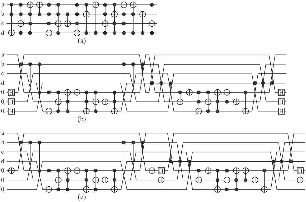
Example 1.
Illustrated in Figure 5(a) is a circuit that we simplify using the suggested approach. The initial circuit contains 4 two-qubit gates, 4 3-qubit gates and 8 4-qubit gates. Using a single number cost estimation introduced in the next section, this circuit requires 144 two-qubit gates. The algorithm, as described, finds two subcircuits sharing control variable in the first and control variable in the second. Those subcircuits are implemented on a separate 3-qubit register and copied in when required, as shown in Figure 5(b). The new circuit contains 10 single-qubit gates, 4 two-qubit gates, and 20 3-qubits gates. In other words, its implementation requires 104 two-qubit gates. To construct the bottom circuit illustrated in Figure 5, one needs to notice that is a fixed point of the function computed by the first subcircuit (after control is factored out), and the second subcircuit (once control is cut) fixes the Boolean cube .

Example 2.
As an example with shared multicontrols consider the circuit cycle10_2 [6] shown in Figure 6(a). As can be seen, the circuit has several gates with shared common controls. According to the proposed algorithm, in this case, one of the auxiliary qubits should be used to collect the product defined by the shared multicontrol and to control the application of Fredkin gates. To find the appropriate set of common controls, the cost of the circuit before and after the optimization should be examined. Using the single number cost estimation introduced in the next section, if the first 6 gates in Figure 6(a) are considered as a subcircuit with three shared common controls, the resulting implementation cost will be maximally improved. Similarly, another subcircuit with 6 gates sharing 4 common controls can be recognized and optimized. The resulting improved circuit is shown in Figure 6(b). Altogether, the cost of the original circuit is improved by about 35% (727 vs. 469).
6 Performance and Results
Before we can test the performance of the introduced approach, it is important to establish a metric to define the implementation cost of a circuit before and after simplification.
6.1 Circuit Cost
With our approach, we allow auxiliary qubits, which directly affects the cost of multiple control gates. Further, we allow those qubits to carry value , which also affects how efficiently one is able to implement multiple control gates. Due to these changes from convention, most common circuit cost metrics used, e.g., [6, 8, 12], cannot be applied. As a result, it is necessary to revisit the circuit cost metric.
Particulars of the definition of the cost metric largely affect practical efficiency. We thus consider a very generic definition of the circuit cost, and suggest that it is re-evaluated in the scenario when circuit costs may be calculated with a better accuracy, and our algorithm/implementation is updated correspondingly.
We will evaluate circuit implementation cost via estimating the number of two-qubit gates required to implement it.
We ignore single-qubit gates partially because they may be merged into two-qubit gates (for instance, in an Ising Hamiltonian22 2 For the purpose of this paper, it suffices to state that an Ising Hamiltonian is such that the two-qubit interaction terms are described by the formula , where is the Pauli-Z matrix acting on qubit , and each is a constant. [11] CNOTNOT may be implemented as efficiently as CNOT, and CNOT is more efficient than CNOT on it own), and partially because they are relatively easy to implement as compared to the two-qubit gates.
Efficiency of the implementation of the two-qubit gates depends on the Hamiltonian describing the physical system being used. For instance, in an Ising Hamiltonian, and up to single-qubit gates, CNOT is equivalent to a single use of the two-qubit interaction term, . With Ising Hamiltionian, SWAP requires three uses of the interaction term, which is a maximum for the number of times an interaction term needs to be used to implement any two-qubit gate in any Hamiltonian [20]. However, if the underlying Hamiltonian is Heisenberg/exchange type [11, 19], SWAP is implemented with a single use of the two-qubit interaction, , and CNOT is notably more complex than SWAP. For the sake of simplicity, we count all two-qubit gates as having the same cost, and assign this cost a value of 1.
Efficient decomposition of the Toffoli and Fredkin gates into a sequence of two-qubit gates largely depends on what physical system is being used. A Toffoli gate may be implemented up to a global phase using at most 3 two-qubit gates (all CNOTs, plus some single-qubit gates) or exactly using 5 two-qubit gates [11]. Other more efficient implementations are possible in very specific cases, e.g., 3 two-qubit gates suffice when the output is computed onto a qutrit (as opposed to a qubit) [14]. The best known implementation of the Fredkin gate requires 3 pulses, each of which is a two-qubit gate [4]. Finally, since when conjugated from left and right by a proper CNOT gate, a Toffoli gate becomes a Fredkin gate, and a Fredkin gate becomes a Toffoli gate, their two-qubit gate implementation costs are within of each other. For the purpose of this paper, we will assign a cost of 5 to both Toffoli and Fredkin gates (minimal two-qubit implementation cost reported in the literature plus 2). Any other number between 3 and 7 would have been reasonable too.

Multiple control Toffoli and multiple control Fredkin gates may be simulated such as shown in Figure 7. As such, both -qubit Toffoli and -qubit Fredkin gates () require 3-qubit Toffoli and Fredkin gates each, which translates into two-qubit gates. Since we ignore single-qubit gates, multiple control Toffoli and Fredkin gates with negated controls have the same cost as their alternatives with positive controls.
6.2 Benchmarks
We have experimented with those MCNC benchmarks we were able to find, and those circuits available at [6]. Reversible circuits for some MCNC benchmarks were reported in [10] (top third of Table 1), and for the most popular that were not explicitly reported in [10] (middle third of Table 1), we used EXORCISM-4 [9] to synthesize them. Finally, we included circuits from [6] (bottom third of Table 1). To save space, we report simplification of only those circuits that were the best reported in the literature at the time of this writing; e.g., [10] reports a circuit for function , however, a better circuit exploiting the fact that this function is symmetric is known [6]. Similarly, we found a number of simplifications in the type circuits, however, we do not report those since efficient circuits for this family of functions have been found [6]. Our approach is most efficient when applied to the circuits with a large proportion of multiple controlled gates. Consequently, we did not find simplifications in the circuits dominated by small gates.
Table 1 reports the results. The first column lists a circuit index number that is introduced to be used in Table 2 as a reference. The next two columns describe the original benchmark function, including its name (name), and the number of inputs and outputs (I/O). The next four columns describe the best known reversible circuit implementations. The first column, # qubits, lists the number of actual qubits used, assuming every multiple control Toffoli gate is implemented most efficiently using a number of auxiliary qubits (Figure 7). This is why this number is higher than the sum of inputs and outputs for irreversible specifications, and the number of inputs/outputs for reversible specifications. The next column, # rev. gates, lists the number of multiple control reversible gates used, cost shows the cost, as defined in Subsection 6.1, i.e., the number of two-qubit gates required, and source shows where or how this circuit may be obtained. The following four columns summarize our simplification results, including the number of actual qubits required in the simplified circuits, the number of gates in the new designs (# quant. gates - # rev. gates = number of Hadamard and Fredkin gates our algorithm introduces), and cost of the simplified circuits. Finally, the last column, % improvement, shows the percentage of the reduction in cost as a result of the application of our algorithm.
Table 2 presents the distribution of the number of gates in the circuits efore and fter simplification. Each circuit is marked with , where is the circuit index number taken from Table 1, and takes values and , to distinguish circuits efore and fter the simplification. Columns report the gate counts used in the corresponding circuit designs. The columns are marked to represent the gate types used: NOT (T1), CNOT (T2), Toffoli (T3), …, Toffoli-21 (T21), Fredkin (F3), and Hadamard (H).
Most circuits were analyzed and simplified almost instantly. The runtime depends primarily on the number of gates, and the complexity of combinations of shared control configurations. The longest computation took 323 seconds (user time) to analyze circuit for function with 5131 gates. It took 25 seconds for the second largest circuit with 1917 gates, implementing the benchmark function . We did not attempt to optimize our implementation.
| Function | Best Known Implementation | After Optimization | % | |||||||
| ckt# | name | I/O | # qubits | # rev. gates | cost | source | # qubits | # quant. gates | cost | improvement |
| 1 | 5xp1 | 7/10 | 22 | 61 | 1177 | [10] | 32 | 141 | 927 | 21.24% |
| 2 | add6 | 12/7 | 24 | 188 | 6120 | [10] | 40 | 330 | 3551 | 41.98% |
| 3 | b12 | 15/9 | 30 | 43 | 1199 | [10] | 41 | 113 | 831 | 30.17% |
| 4 | clip | 9/5 | 21 | 120 | 5412 | [10] | 31 | 296 | 2924 | 45.97% |
| 5 | in7 | 26/10 | 51 | 70 | 4228 | [10] | 65 | 190 | 2287 | 45.91% |
| 6 | life | 9/1 | 17 | 50 | 2480 | [10] | 24 | 152 | 1870 | 24.6% |
| 7 | ryy6 | 16/1 | 30 | 40 | 2686 | [10] | 40 | 134 | 1737 | 35.33% |
| 8 | sao2 | 10/4 | 22 | 58 | 3972 | [10] | 30 | 164 | 1806 | 54.53% |
| 9 | seq | 41/35 | 94 | 1917 | 188827 | [10] | 113 | 2239 | 84284 | 55.36% |
| 10 | t481 | 16/1 | 19 | 13 | 220 | [10] | 19 | 13 | 220 | 0% |
| 11 | vg2 | 25/8 | 51 | 207 | 16525 | [10] | 76 | 543 | 11709 | 29.14% |
| 12 | z4 | 7/4 | 14 | 36 | 512 | [10] | 20 | 78 | 484 | 5.47% |
| 13 | apex4 | 9/19 | 35 | 5131 | 228015 | [9] | 61 | 5409 | 170541 | 25.21% |
| 14 | apla | 10/12 | 29 | 70 | 3390 | [9] | 40 | 244 | 1709 | 49.59% |
| 15 | bbm | 4/4 | 10 | 16 | 224 | [9] | 17 | 42 | 164 | 26.79% |
| 16 | co14 | 14/1 | 26 | 14 | 1610 | [9] | 32 | 60 | 1070 | 33.54% |
| 17 | cordic | 23/2 | 40 | 1546 | 188715 | [9] | 57 | 1686 | 127615 | 32.38% |
| 18 | cu | 14/11 | 33 | 27 | 1110 | [9] | 39 | 93 | 631 | 43.15% |
| 19 | decod | 16/5 | 24 | 83 | 1931 | [9] | 41 | 193 | 847 | 56.14% |
| 20 | f51m | 14/8 | 34 | 369 | 25155 | [9] | 52 | 523 | 21953 | 12.73% |
| 21 | root | 8/5 | 19 | 67 | 2605 | [9] | 27 | 185 | 1786 | 31.44% |
| 22 | sqr6 | 6/12 | 22 | 59 | 955 | [9] | 30 | 109 | 655 | 31.41% |
| 23 | sqrt8 | 8/4 | 17 | 27 | 495 | [9] | 21 | 67 | 405 | 18.18% |
| 24 | table3 | 14/14 | 40 | 802 | 74530 | [9] | 63 | 1578 | 30320 | 59.32% |
| 25 | cycle10_2 | 12/12 | 20 | 19 | 727 | [6] | 22 | 59 | 469 | 35.49% |
| 26 | cycle17_3 | 20/20 | 35 | 48 | 3388 | [6] | 38 | 164 | 1824 | 46.16% |
| 27 | mod1024adder | 20/20 | 28 | 55 | 1435 | [6] | 30 | 139 | 1011 | 29.55% |
| 28 | mod1048576adder | 40/40 | 58 | 210 | 12090 | [6] | 59 | 588 | 6485 | 46.36% |
| 29 | nth_prime6_inc | 6/6 | 9 | 55 | 592 | [6] | 14 | 75 | 583 | 1.52% |
7 Advantages and Limitations
The control reduction algorithm we introduced in this paper has the following practical advantages and limitations.
- 1.
Advantages:
- •
- •
This algorithm is particularly useful in compiling the Boolean if-then-else type statement in a quantum programming language (previously mentioned in [16]). Indeed, the statement if then else can be implemented such as shown in Figure 8. The bottom circuit allows execution of statements and in parallel, which may be particularly helpful in the scenario when , , and have relatively high implementation costs, and a faster implementation is preferred.
Figure 8: Implementation of the if then else statement. Top: five basic ways to implement this statement. Circuit equivalence from Figure 3 may be applied to simplify each of these five implementations. Middle to bottom: an illustration of how the circuit equivalence from Figure 3 helps to simplify the top right implementation.
- 2.
Limitations:
- •
- •
A sufficient number of auxiliary qubits set to value needs to be made available for the algorithm to work efficiently. However, the performance improves as the number of auxiliary qubits carrying value grows (for example, we did not test nested application of our algorithm, but expect the results may improve compared to those reported in this paper).
| ckt# | T1 | T2 | T3 | T4 | T5 | T6 | T7 | T8 | T9 | T10 | T11 | T12 | T13 | T14 | T15 | T16 | T17 | T18 | T19 | T20 | T21 | F3 | H |
|---|---|---|---|---|---|---|---|---|---|---|---|---|---|---|---|---|---|---|---|---|---|---|---|
| 1b | 0 | 17 | 7 | 12 | 10 | 4 | 5 | 6 | 0 | 0 | 0 | 0 | 0 | 0 | 0 | 0 | 0 | 0 | 0 | 0 | 0 | 0 | 0 |
| 1a | 0 | 27 | 20 | 10 | 4 | 7 | 1 | 0 | 0 | 0 | 0 | 0 | 0 | 0 | 0 | 0 | 0 | 0 | 0 | 0 | 0 | 52 | 20 |
| 2b | 6 | 0 | 23 | 18 | 29 | 35 | 45 | 32 | 0 | 0 | 0 | 0 | 0 | 0 | 0 | 0 | 0 | 0 | 0 | 0 | 0 | 0 | 0 |
| 2a | 19 | 16 | 47 | 37 | 45 | 32 | 0 | 0 | 0 | 0 | 0 | 0 | 0 | 0 | 0 | 0 | 0 | 0 | 0 | 0 | 0 | 100 | 34 |
| 3b | 5 | 0 | 6 | 4 | 9 | 4 | 9 | 6 | 0 | 0 | 0 | 0 | 0 | 0 | 0 | 0 | 0 | 0 | 0 | 0 | 0 | 0 | 0 |
| 3a | 8 | 1 | 13 | 11 | 11 | 2 | 1 | 0 | 0 | 0 | 0 | 0 | 0 | 0 | 0 | 0 | 0 | 0 | 0 | 0 | 0 | 42 | 24 |
| 4b | 0 | 2 | 10 | 2 | 7 | 14 | 33 | 28 | 16 | 8 | 0 | 0 | 0 | 0 | 0 | 0 | 0 | 0 | 0 | 0 | 0 | 0 | 0 |
| 4a | 0 | 9 | 39 | 38 | 31 | 12 | 2 | 3 | 0 | 0 | 0 | 0 | 0 | 0 | 0 | 0 | 0 | 0 | 0 | 0 | 0 | 140 | 22 |
| 5b | 4 | 3 | 5 | 4 | 3 | 0 | 3 | 5 | 13 | 10 | 9 | 2 | 2 | 4 | 1 | 0 | 0 | 2 | 0 | 0 | 0 | 0 | 0 |
| 5a | 9 | 7 | 8 | 11 | 15 | 13 | 3 | 2 | 5 | 1 | 0 | 0 | 2 | 0 | 0 | 0 | 0 | 0 | 0 | 0 | 0 | 78 | 36 |
| 6b | 0 | 0 | 0 | 0 | 3 | 9 | 15 | 10 | 11 | 2 | 0 | 0 | 0 | 0 | 0 | 0 | 0 | 0 | 0 | 0 | 0 | 0 | 0 |
| 6a | 0 | 0 | 10 | 17 | 11 | 9 | 12 | 1 | 0 | 0 | 0 | 0 | 0 | 0 | 0 | 0 | 0 | 0 | 0 | 0 | 0 | 76 | 16 |
| 7b | 0 | 1 | 0 | 3 | 0 | 6 | 0 | 9 | 0 | 9 | 0 | 7 | 0 | 4 | 0 | 1 | 0 | 0 | 0 | 0 | 0 | 0 | 0 |
| 7a | 3 | 2 | 7 | 7 | 7 | 10 | 1 | 6 | 0 | 4 | 0 | 1 | 0 | 0 | 0 | 0 | 0 | 0 | 0 | 0 | 0 | 60 | 26 |
| 8b | 0 | 2 | 1 | 0 | 0 | 0 | 0 | 3 | 17 | 28 | 7 | 0 | 0 | 0 | 0 | 0 | 0 | 0 | 0 | 0 | 0 | 0 | 0 |
| 8a | 0 | 6 | 6 | 30 | 9 | 10 | 4 | 2 | 1 | 0 | 0 | 0 | 0 | 0 | 0 | 0 | 0 | 0 | 0 | 0 | 0 | 78 | 18 |
| 9b | 0 | 2 | 14 | 1 | 0 | 8 | 2 | 33 | 128 | 187 | 115 | 126 | 189 | 151 | 209 | 245 | 198 | 141 | 76 | 52 | 40 | 0 | 0 |
| 9a | 19 | 69 | 204 | 194 | 237 | 213 | 168 | 283 | 184 | 171 | 100 | 53 | 40 | 0 | 0 | 0 | 0 | 0 | 0 | 0 | 0 | 252 | 52 |
| 10b | 1 | 0 | 4 | 0 | 8 | 0 | 0 | 0 | 0 | 0 | 0 | 0 | 0 | 0 | 0 | 0 | 0 | 0 | 0 | 0 | 0 | 0 | 0 |
| 10a | 1 | 0 | 4 | 0 | 8 | 0 | 0 | 0 | 0 | 0 | 0 | 0 | 0 | 0 | 0 | 0 | 0 | 0 | 0 | 0 | 0 | 0 | 0 |
| 11b | 0 | 0 | 4 | 7 | 16 | 12 | 10 | 16 | 8 | 24 | 30 | 26 | 16 | 16 | 4 | 4 | 0 | 4 | 6 | 0 | 4 | 0 | 0 |
| 11a | 0 | 14 | 33 | 28 | 12 | 20 | 10 | 28 | 26 | 18 | 18 | 4 | 4 | 0 | 0 | 6 | 0 | 4 | 0 | 0 | 0 | 264 | 54 |
| 12b | 0 | 2 | 14 | 10 | 6 | 4 | 0 | 0 | 0 | 0 | 0 | 0 | 0 | 0 | 0 | 0 | 0 | 0 | 0 | 0 | 0 | 0 | 0 |
| 12a | 0 | 4 | 26 | 10 | 0 | 2 | 0 | 0 | 0 | 0 | 0 | 0 | 0 | 0 | 0 | 0 | 0 | 0 | 0 | 0 | 0 | 26 | 10 |
| 13b | 0 | 0 | 0 | 171 | 537 | 1188 | 1460 | 1167 | 504 | 104 | 0 | 0 | 0 | 0 | 0 | 0 | 0 | 0 | 0 | 0 | 0 | 0 | 0 |
| 13a | 8 | 1 | 165 | 651 | 1265 | 1520 | 1072 | 367 | 86 | 0 | 0 | 0 | 0 | 0 | 0 | 0 | 0 | 0 | 0 | 0 | 0 | 222 | 52 |
| 14b | 0 | 0 | 0 | 6 | 5 | 7 | 16 | 18 | 13 | 5 | 0 | 0 | 0 | 0 | 0 | 0 | 0 | 0 | 0 | 0 | 0 | 0 | 0 |
| 14a | 3 | 24 | 25 | 11 | 12 | 3 | 2 | 4 | 0 | 0 | 0 | 0 | 0 | 0 | 0 | 0 | 0 | 0 | 0 | 0 | 0 | 136 | 24 |
| 15b | 0 | 4 | 4 | 0 | 8 | 0 | 0 | 0 | 0 | 0 | 0 | 0 | 0 | 0 | 0 | 0 | 0 | 0 | 0 | 0 | 0 | 0 | 0 |
| 15a | 2 | 4 | 10 | 0 | 2 | 0 | 0 | 0 | 0 | 0 | 0 | 0 | 0 | 0 | 0 | 0 | 0 | 0 | 0 | 0 | 0 | 12 | 12 |
| 16b | 0 | 0 | 0 | 0 | 0 | 0 | 0 | 0 | 0 | 0 | 0 | 0 | 0 | 14 | 0 | 0 | 0 | 0 | 0 | 0 | 0 | 0 | 0 |
| 16a | 0 | 0 | 0 | 12 | 0 | 0 | 0 | 0 | 0 | 0 | 6 | 0 | 0 | 2 | 0 | 0 | 0 | 0 | 0 | 0 | 0 | 30 | 10 |
| 17b | 1 | 0 | 0 | 0 | 0 | 5 | 0 | 0 | 0 | 0 | 0 | 388 | 0 | 0 | 768 | 0 | 384 | 0 | 0 | 0 | 0 | 0 | 0 |
| 17a | 1 | 0 | 3 | 2 | 4 | 2 | 0 | 388 | 0 | 0 | 768 | 0 | 384 | 0 | 0 | 0 | 0 | 0 | 0 | 0 | 0 | 92 | 42 |
| 18b | 1 | 0 | 2 | 0 | 7 | 4 | 5 | 4 | 0 | 0 | 4 | 0 | 0 | 0 | 0 | 0 | 0 | 0 | 0 | 0 | 0 | 0 | 0 |
| 18a | 8 | 6 | 6 | 0 | 9 | 2 | 2 | 0 | 0 | 0 | 0 | 0 | 0 | 0 | 0 | 0 | 0 | 0 | 0 | 0 | 0 | 42 | 18 |
| 19b | 0 | 1 | 8 | 12 | 46 | 16 | 0 | 0 | 0 | 0 | 0 | 0 | 0 | 0 | 0 | 0 | 0 | 0 | 0 | 0 | 0 | 0 | 0 |
| 19a | 8 | 17 | 50 | 12 | 2 | 0 | 0 | 0 | 0 | 0 | 0 | 0 | 0 | 0 | 0 | 0 | 0 | 0 | 0 | 0 | 0 | 70 | 34 |
| 20b | 0 | 0 | 9 | 16 | 22 | 27 | 26 | 23 | 47 | 46 | 60 | 59 | 23 | 6 | 5 | 0 | 0 | 0 | 0 | 0 | 0 | 0 | 0 |
| 20a | 4 | 8 | 29 | 25 | 21 | 27 | 21 | 47 | 46 | 60 | 59 | 23 | 6 | 5 | 0 | 0 | 0 | 0 | 0 | 0 | 0 | 106 | 36 |
| 21b | 0 | 5 | 6 | 2 | 11 | 6 | 11 | 13 | 13 | 0 | 0 | 0 | 0 | 0 | 0 | 0 | 0 | 0 | 0 | 0 | 0 | 0 | 0 |
| 21a | 1 | 6 | 22 | 20 | 13 | 16 | 1 | 0 | 0 | 0 | 0 | 0 | 0 | 0 | 0 | 0 | 0 | 0 | 0 | 0 | 0 | 88 | 18 |
| 22b | 0 | 5 | 24 | 12 | 1 | 14 | 3 | 0 | 0 | 0 | 0 | 0 | 0 | 0 | 0 | 0 | 0 | 0 | 0 | 0 | 0 | 0 | 0 |
| 22a | 2 | 5 | 37 | 17 | 1 | 1 | 0 | 0 | 0 | 0 | 0 | 0 | 0 | 0 | 0 | 0 | 0 | 0 | 0 | 0 | 0 | 30 | 16 |
| 23b | 0 | 5 | 7 | 4 | 4 | 3 | 3 | 1 | 0 | 0 | 0 | 0 | 0 | 0 | 0 | 0 | 0 | 0 | 0 | 0 | 0 | 0 | 0 |
| 23a | 0 | 5 | 13 | 11 | 2 | 0 | 0 | 0 | 0 | 0 | 0 | 0 | 0 | 0 | 0 | 0 | 0 | 0 | 0 | 0 | 0 | 24 | 12 |
| 24b | 0 | 0 | 0 | 0 | 6 | 10 | 0 | 10 | 61 | 89 | 154 | 169 | 154 | 110 | 39 | 0 | 0 | 0 | 0 | 0 | 0 | 0 | 0 |
| 24a | 6 | 55 | 73 | 120 | 189 | 143 | 105 | 73 | 24 | 36 | 16 | 4 | 2 | 0 | 0 | 0 | 0 | 0 | 0 | 0 | 0 | 684 | 48 |
| 25b | 0 | 2 | 2 | 2 | 2 | 2 | 2 | 2 | 2 | 2 | 1 | 0 | 0 | 0 | 0 | 0 | 0 | 0 | 0 | 0 | 0 | 0 | 0 |
| 25a | 2 | 4 | 4 | 4 | 5 | 4 | 0 | 0 | 0 | 0 | 0 | 0 | 0 | 0 | 0 | 0 | 0 | 0 | 0 | 0 | 0 | 24 | 12 |
| 26b | 0 | 3 | 3 | 3 | 3 | 3 | 3 | 3 | 3 | 3 | 3 | 3 | 3 | 3 | 3 | 3 | 2 | 1 | 0 | 0 | 0 | 0 | 0 |
| 26a | 6 | 9 | 9 | 12 | 5 | 3 | 3 | 5 | 7 | 1 | 0 | 0 | 0 | 0 | 0 | 0 | 0 | 0 | 0 | 0 | 0 | 84 | 20 |
| 27b | 0 | 10 | 9 | 8 | 7 | 6 | 5 | 4 | 3 | 2 | 1 | 0 | 0 | 0 | 0 | 0 | 0 | 0 | 0 | 0 | 0 | 0 | 0 |
| 27a | 6 | 16 | 16 | 15 | 10 | 4 | 0 | 0 | 0 | 0 | 0 | 0 | 0 | 0 | 0 | 0 | 0 | 0 | 0 | 0 | 0 | 60 | 12 |
| 28b | 0 | 20 | 19 | 18 | 17 | 16 | 15 | 14 | 13 | 12 | 11 | 10 | 9 | 8 | 7 | 6 | 5 | 4 | 3 | 2 | 1 | 0 | 0 |
| 28a | 25 | 45 | 47 | 47 | 35 | 20 | 15 | 8 | 10 | 6 | 2 | 0 | 0 | 0 | 0 | 0 | 0 | 0 | 0 | 0 | 0 | 308 | 20 |
| 29b | 5 | 12 | 14 | 11 | 11 | 2 | 0 | 0 | 0 | 0 | 0 | 0 | 0 | 0 | 0 | 0 | 0 | 0 | 0 | 0 | 0 | 0 | 0 |
| 29a | 6 | 13 | 15 | 9 | 11 | 1 | 0 | 0 | 0 | 0 | 0 | 0 | 0 | 0 | 0 | 0 | 0 | 0 | 0 | 0 | 0 | 10 | 10 |
8 Conclusions
In this paper, we presented an approach for systematic optimization of reversible circuits that trades in qubits to achieve a lower implementation cost. This may be of particular interest in practice when a multistage quantum algorithm (including computations in the Boolean domain) needs to be executed on a quantum processor, and there are a number of scrap qubits available to be used to optimize intermediate computations. The proposed approach may be extended to optimize quantum controlled transformations.
9 Acknowledgments
This article was based on work partially supported by the National Science Foundation, during D. Maslov’s assignment at the Foundation.
References
- [1] S. Aaronson and D. Gottesman. Improved simulation of stabilizer circuits. Physical Review A, 70(052328), 2004, http://arxiv.org/abs/quant-ph/0406196.
- [2] A. Barenco, C. H. Bennett, R. Cleve, D. P. DiVinchenzo, N. Margolus, P. Shor, T. Sleator, J. A. Smolin, and H. Weinfurter. Elementary gates for quantum computation. Physical Review A, 52:3457–3467, 1995, http://arxiv.org/abs/quant-ph/9503016.
- [3] D. Deutsch and R. Jozsa. Rapid solutions of problems by quantum computation. Proceedings of the Royal Society of London A, 439(553), 1992.
- [4] X. Fei, D. Jiangfeng, S. Mingjun, Z. Xianyi, H. Rongdian, and W. Jihui. Realization of the Fredkin gate by three transition pulses in a nuclear magnetic resonance quantum information processor. Chinese Phys. Lett., 19(8):1048-1050, 2002, http://arxiv.org/abs/quant-ph/0202014.
- [5] A. Kitaev. “Quantum measurements and the Abelian Stabilizer Problem”, 1995, http://arxiv.org/abs/quant-ph/9511026.
- [6] D. Maslov. Reversible Logic Synthesis Benchmarks Page. http://webhome.cs.uvic.ca/~ dmaslov/, last accessed June 2010.
- [7] D. Maslov, D. M. Miller, and G. W. Dueck. Toffoli network synthesis with templates. IEEE Transactions on CAD, 24(6):807–817, 2005.
- [8] D. Maslov, D. M. Miller, and G. W. Dueck. Techniques for the synthesis of reversible Toffoli networks. ACM Transactions on Design Automation of Electronic Systems, 12(4), article 42, 2007, http://arxiv.org/abs/quant-ph/0607166.
- [9] A. Mishchenko. EXORCISM-4. http://web.cecs.pdx.edu/~ al anmi/research/min/minEsop.htm, last accessed June 2010.
- [10] A. Mishchenko and M. Perkowski. “Logic synthesis of reversible wave cascades”. In Proc. International Workshop on Logic Synthesis, pages 197-202, June 2002.
- [11] M. Nielsen and I. Chuang. Quantum Computation and Quantum Information. Cambridge University Press, 2000.
- [12] A. K. Prasad, V. V. Shende, K. N. Patel, I. L. Markov, and J. P. Hayes. Algorithms and data structures for simplifying reversible circuits. ACM Journal of Emerging Technologies in Computing Systems, 2(4):277-293, 2006.
- [13] J. Proos and C. Zalka. Shor’s discrete logarithm quantum algorithm for elliptic curves. Quantum Information and Computation, 3(4):317–344, 2003, http://arxiv.org/abs/quant-ph/0301141.
- [14] T. C. Ralph, K. J. Resch, and A. Gilchrist. Efficient Toffoli gates using qudits. Physical Review A, 75(022313), 2007, http://arxiv.org/abs/0806.0654.
- [15] M. Saeedi, M. S. Zamani, M. Sedighi, and Z. Sasanian. Reversible circuit synthesis using a cycle-based approach. ACM Journal of Emerging Technologies in Computing Systems, 6(4), article 13, 2010, http://arxiv.org/abs/1004.4320.
- [16] V. V. Shende, A. K. Prasad, I. L. Markov, and J. P. Hayes. Synthesis of Reversible Logic Circuits. IEEE Transactions on CAD, 22(6):710–722, 2003.
- [17] http://en.wikipedia.org/wiki/Cycles_and_fixed_points, last accessed June 2010.
- [18] R. Wille and R. Drechsler. BDD-based synthesis of reversible logic for large functions. In Proc. Design Automation Conference, pages 270–275, 2009.
- [19] S. A. Wolf, D. D. Awschalom, R. A. Buhrman, J. M. Daughton, S. von Molnar, M. L. Roukes, A. Y. Chtchelkanova, and D. M. Treger. Spintronics: A Spin-Based Electronics Vision for the Future. Science 294(5546):1488–1495, November 2001.
- [20] J. Zhang, J. Vala, S. Sastry, and K. B. Whaley. Geometric theory of nonlocal two-qubit operations. Physical Review A, 67(042313), April 2003, http://arxiv.org/abs/quant-ph/0209120.