Comment on ”Bound states of edge dislocations: The quantum dipole problem in two dimensions”
Abstract
We show that it is possible to improve some of the numerical results contained in a recent paper with an optimal implementation of the methods used in that paper. A careful analysis done using the Rayleigh-Ritz method provides a rigorous upper bound for the energy of the ground state of an electron in a two dimensional potential generated by the edge dislocation, as well as precise values for the excited states. The extrapolation of the results corresponding to different subspaces is used to obtain an alternative estimate of the fundamental energy of the model. The energies of the first 500 states that we have calculated are in perfect agreement with the expected asymptotic behavior.
pacs
67.80.B-, 02.60.-xThe presence of edge dislocations in a solid may have strong effects on the mechanical, transport, elastic and superconducting properties of the solid [1]. The knowledge of the spectrum of the bound states at the edge is therefore helpful to assess the change in the properties of the material.
With this motivation, the authors of a recent paper, ref. [1], have considered the Schrödinger equation (SE) for an electron confined in a two dimensions and subject to a potential (corresponding to a straight dislocation along the -axis):
| (1) |
Unfortunately this equation is not exactly solvable and its solution requires approximate methods. In effect ref. [1] provides a detailed list of the different approaches which have been applied in the literature to this problem [2, 3, 5, 4, 6, 7]: the numerical estimates for the energy of the ground state obtained in these works are reported in Table 1 of ref.[1] in units of . The last result of the table is the improved estimate obtained in that paper discretizing the Schrödinger equation on a uniform square grid and working with matrices of a maximum size of . The authors quote an error of for the numerical eigenvalues of the planar Coulomb problem, whose exact solutions are known [8]. Unfortunately, since the precision of the results depends on the specific problem considered, the accuracy of the numerical results of ref. [1] is not granted for the dipole problem and actually one may expect on qualitative grounds larger errors for the quantum dipole problem, due to the dependence on in the potential.
In both cases, the long range nature of the potential and its singular behavior at would better be taken into account using a nonuniform two-dimensional grid (see refs. [9, 10] for a discussion of collocation methods with nonuniform grids).
A second difficulty of the computational approach based on the discretization of the Schrödinger equation, which is mentioned in ref. [1], is the limited number of states which can be obtained with acceptable precision with a given grid, due to the different length scales of the excited states: as a result the estimates for the first few states of the dipole potential cannot be equally accurate. Finally, one should bear in mind that the discretization of the SE, however accurate it could be, does not provide upper bounds on the energy of the fundamental mode: the result obtained in ref. [1] may thus either over or underestimate the exact energy.
The second approach discussed by the authors of ref.[1] is what they call a ”Coulomb basis method”, which is essentially a Rayleigh-Ritz (RR) approach which uses the basis of the planar Coulomb problem (see ref. [8]). The Rayleigh-Ritz approach, in contrast to the real-space diagonalization method mentioned earlier, does provide an upper bound to the energy of the fundamental state and a direct decomposition of the approximate solutions in the basis chosen. Unfortunately the potentialities of this method have not been fully exploited in that paper: the main purpose of this Comment is then to obtain stricter bounds for the energy of the ground state working with a larger set of functions.
The angular and radial parts respectively read 11 1 Notice the typo in the bounds over in eq.(5) of ref. [1].
and
| (7) | |||||
where . Here is the confluent hypergeometric function.
The bound state energies of the 2D hydrogen are simply [8]
| (8) |
The RR approach requires the calculation of the matrix elements of the Hamiltonian of eq. (1) in the basis (2):
where
The evaluation of the radial integral is not straightforward as in the case of the angular integrals but it can also be done analytically. Defining and ( ), the confluent hypergeometric functions in this integral reduce to polynomials of degrees and respectively, for and positive integers. The original integral is therefore reduced to a sum of integrals which can be done explicitly:
| (9) |
where the are the Pochhammer symbols and
| (10) | |||||
| (11) | |||||
The authors of ref.[1] have used the analytical expressions for these integrals, although they had to restrict their calculation to a set of basis functions, corresponding to and , due to the numerical round-off errors that become important for the matrix elements corresponding to larger quantum numbers. In our numerical calculation we have used Mathematica 8 [11], obtaining symbolic expressions for the matrix elements, which were then evaluated numerically avoiding the round-off errors which would appear in a fully numerical calculation.
It is convenient to introduce the notation and regard as a variational parameter controlling the length scale. We then rewrite the matrix elements of the Hamiltonian making the dependence upon explicit:
| (12) | |||||
This is precisely the approach followed by Dasbiswas et al. in ref. [1], who observe that the bound for the ground state energy obtained for is not good: after minimizing with respect to they obtain an improved bound working with states (we adopt their convention of reporting the energies in units of ).
Interestingly, these authors use the original basis () for the excited states, claiming that ”the real-space diagonalization methods provide a better estimate of the ground-state energy whereas the Coulomb basis method is more suitable for higher excited states.” It is not clear on what grounds this statement is made and actually we will show in this Comment that the choice of calculating the excited states for is far from optimal. We will also obtain an alternative estimate for the energy of the ground state of the quantum dipole problem, which falls above the one calculated in ref. [1].
Our first observation concerns the number of bound states which are obtained in the calculation at a given : while for there are bound states, for (corresponding to the minimum of ) there are just 3 bounds states. This behavior should not surprise us, since determines the radial length scale of the wave function, and different states have different range: the fact that for a large fewer bound states are present, simply tells us that the physical states which are not captured by the calculation have a larger range. Therefore, if one wants to estimate a few excited states, one needs to calculate these states using different values of to account for the different length scales of each state.
The fundamental question is therefore how to choose : if the problem under consideration has certain symmetries, which are also symmetries of the basis, then the variational principle applied to a trial wave function with that symmetry will provide again an upper bound to the lowest mode in that symmetry class: for our problem this is the case of functions which are odd with respect to the change . For the remaining states, the eigenvalues of the RR matrix will vary with , without providing a variational bound. However, if we consider a given state, its exact energy and wave function will be independent of , which is an unphysical parameter of the basis. As such, we may argue that the optimal value of (and correspondingly the most accurate value for the energy) will be the one for which the calculated eigenvalue is less sensitive to changes of . This is the essence of the ”principle of minimal sensitivity” (PMS) [12]. We will soon use the PMS to calculate the excited states of eq. (1).
We now proceed to illustrate our numerical results, concentrating for the moment on the ground state.


In the first plot of Fig.1 we show the variational bound for the ground state energy of eq.(1) as a function of the maximum quantum number used in the RR method (we have considered even values of ). For a given , the portion of Hilbert space used in the calculation contains states (the results obtained by Dasbiswas et al., for instance, correspond to and therefore to a matrix). For each value of we have selected the value of for which the corresponding is minimal; the numerical calculation is stopped when the convergence on the first digits of was reached.
Remarkably these data display a very regular behavior, which is well described by the fit
| (13) |
In the second plot of Fig.1 we show the values for the ground state energy obtained repeatedly using the Shanks transformation on the sets of the energies of the first plot. The index in the horizontal axis indicates to the number of consecutive Shanks transformations used, while the value on the vertical axis is the corresponding result obtained with the Shanks transformations, involving the values corresponding to largest . These values seem to converge to the value . The horizontal line corresponds to the constant value reached by eq. (13) for . Notice the disagreement of our results with the value obtained in ref. [1], . Being fair, there is no rigorous criterion granting that our result is more precise, although the extrapolation of very regular sequences of numbers typically provides very accurate estimates.
The behavior of the optimal obtained with the PMS at different is described very well by the a cubic fit . There is a clear physical justification of the behavior of , which grows with : as the number of states in the calculation is increased, one can use a basis with shorter length scale (i.e. larger ) to build the approximate eigenfunctions of the problem.
Although we believe that the values of that we have obtained with the fit (13) or with the Shanks transformation are more precise than the result obtained in ref. [1], we are aware that the extrapolation of the values of do not themselves fulfill a variational bound. In other words, we may expect them to be closer to the exact value, but we cannot be sure that they fall above it. We will now show that it is possible to obtain stricter bounds on , even working with less states. As we have mentioned before, the largest set of states used in Fig.1 corresponds to , i.e. states ( and ). We may wonder to what extent the results would change by restricting the states to . While one can safely drop the negative values of , since the ground state must be symmetric with respect to , it is not a priori clear the error introduced by using an upper cutoff .
Let be the eigenvector corresponding to the smallest eigenvalue of the matrix obtained in RR approach: the normalization of implies that . Any deviation from 1 of the sum when the components of corresponding to are set to zero will give us an idea of how important these states are for the calculation. For one finds out that this deviation is completely negligible, . To confirm this finding we may compare the lowest eigenvalue of the full matrix, , with the lowest eigenvalue of the reduced matrix, corresponding to , . We have , which is of the same order of the deviation discussed above. The effective dimensionless coupling constant calculated with the wave function corresponding to is , which agrees with the result found in ref.[1], using a simple variational ansatz.
With this result in mind we have built a matrix, corresponding to and , obtaining the bound . Notice that the fit of eq. (13) for provides a result which is very close to this, . We have then built a matrix, corresponding to and , obtaining our most precise bound . Also in this case the fit of eq. (13) for provides a result which is very close to this, .
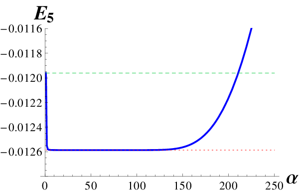
We now discuss the excited states of eq. (1): as we have mentioned earlier there is no valid reason for calculating the excited states at . Fig.4 should convince the reader of this point: here the energy of the fifth state is plotted at different values of , and compared with the value at (dashed line), which corresponds to the choice done in [1]. The dotted line at the bottom corresponds to the minimum of the curve, and it provides the most accurate value for which can be obtained working with a subspace corresponding to . Table 1 illustrates the different results obtained using the two approaches for the first five states. The last column reports the quantity , which provides an estimate of the error done using . Interestingly the values obtained with the PMS for the third and fifth states are close to the ones obtained in ref. [1] using a discretization of the Schrödinger equation: these states correspond to smaller values of , indicating that their length scales are larger than those of the other three states. So, for example, the third state, has a smaller than the fourth state, which is higher in energy. The authors of [1] have also observed a similar behavior for some of the states ( and ) that they have calculated, although they have not given ”any satisfactory explanation for these irregular features”. Our explanation of this phenomenon is simple: if a state with a modest spatial extent has a larger probability density in the region close to (recall that the potential is attractive for ), its energy may be higher than the energy of a state with larger spatial extent but smaller probability density in the region close to .
In Fig. 3 we plot the optimal value of as a function of the level number , obtained using the subspace corresponding to . The assumption used in ref.[1], , is clearly valid only for the higher excited states (). Notice the oscillations of , which signal the presence of contiguous states with different length scales, as mentioned earlier.
In Fig. 4 we have compared the behavior of obtained using either the PMS (solid line) or setting (dashed line), with the asymptotic law of eq.(10) of ref.[1] (dotted line). The plot clearly proves the superiority of the PMS results. This superiority can also be established by looking at the fit of the first 500 values of :
| 1 | -0.0970117 | -0.127886 | 767.132 | 0.137281 |
|---|---|---|---|---|
| 2 | -0.0328379 | -0.0394579 | 294.189 | 0.0915679 |
| 3 | -0.0220914 | -0.0232932 | 137.674 | 0.0264818 |
| 4 | -0.016764 | -0.0193729 | 161.317 | 0.072193 |
| 5 | -0.0119611 | -0.0125862 | 86.4652 | 0.0254668 |


In conclusion, we believe that we have presented numerical results which complement and extend the results of ref. [1]; we have shown that the application of the Rayleigh-Ritz method to this problem provides very accurate results, both exploiting the Shanks transformation and performing the calculation on a selected portion of the Hilbert space. In this way we have calculated the ground state energy corresponding to , working with a matrix of size , instead of the full matrix , obtaining our most precise bound, . Using the numerical results for the excited states, calculated using the PMS, we have reproduced with high accuracy the expected asymptotic behavior of eq.(10) of ref. [1].
Acknowledgements.
The author acknowledges the support of SNI-Conacyt.References
- [1] K. Dasbiswas, D. Goswami, C.D. Yoo and A.T. Dorsey, Phys. Rev.B 81, 064516 (2010)
- [2] R. Landauer, Phys. Rev.94, 1386 (1954)
- [3] P.R.Emtage, Phys. Rev. 163, 865 (1967)
- [4] V.A. Slyusarev and K.A.Chishko, Fiz.Met.Metalloved. 58, 877 (1984)
- [5] V.M. Nabutovskii and B.Ya. Shapiro, JETP Lett. 26, 473 (1977)
- [6] I.M. Dubrovskii, Low Temp. Phys.23, 976 (1997)
- [7] J.L.Farvacque and P.Fracois, Phys.Status Solidi B 223, 635 (2001)
- [8] X.L.Yang, S.H.Guo, F.T.Chan, K.W.Wong and W.Y.Ching, Phys. Rev.A 43, 1186 (1991)
- [9] E. Fattal, R. Baer and R. Kosloff, Phys.Rev. E 53, 1217 (1996)
- [10] J.P.Boyd, Chebyshev and Fourier Spectral Methods: Second Revised Edition, Dover, New York (2001), 688 pp.
- [11] Wolfram Research, Inc., MATHEMATICA Version 8.0 ͑Wolfram Research Inc., Champaign, Illinois, 2010.
- [12] P. M. Stevenson, Phys. Rev. D 23, 2916 (1981)