Microscopic theory of type-1.5 superconductivity in two-band systems
Abstract
We report a self-consistent microscopic theory of characteristic length scales, vortex structure and type-1.5 superconducting state in two-band systems using two-band Eilenberger formalism.
pacs
74.25.QP, 74.25.Fy, 73.40.GkI Introduction
The usual classification of superconductors characterizes materials by the Ginzburg-Landau parameter (which is the ratio of the characteristic length scale of the order parameter variation and the magnetic field penetration length ) [1]. The remarkable property is that within the GL theory of single-component superconductivity determines the major features of the phase diagram of the system in magnetic field. In type-I superconductor (i.e. order parameter is the slowest varying field), vortex excitations have attractive interaction and are thermodynamically unstable in applied magnetic field. Thus in an applied field a type-I system forms macroscopically large normal domains [2]. For (type-II superconductivity) vortices are thermodynamically stable and interact repulsively yielding a new phase in strong magnetic fields: a lattice of quantized vortices [3, 2]. In the Bogomolnyi limit () the vortices do not interact in the Ginzburg-Landau theory. However indeed it should be remarked that going to a deeper microscopic level there are always “next-to-leading order” microscopic corrections. These corrections, though unimportant even slightly away from this limit, provide weak non-universal intervortex interactions when is very close to see e.g. [4, 5]. Apparently a counterpart of this limit is also possible in multi-component systems. However in this case the Bogomolnyi limit could appear only via quite extreme fine-tuning of parameters and therefore is not of much physical relevance. In this work we are interested only in the entirely different physics of intervortex interactions and magnetic response of multicomponent systems originating from the different funamental length scales very far from any counterparts of Bogomolnyi limit.
A question which attracted much attention recently is whether the type-I/type-II classification is sufficient for characterizing the rapidly growing family of multicomponent systems of physical interest [6]. A clear cut example of the system where type-I/type-II dichotomy does not hold is the projected coexistent electronic and protonic (or deuteronic) superconductivity [7] in hydrogen isotopes, their mixtures and hydrogen rich alloys at ultrahigh compression as well as the coexisting protonic and -hyperonic superconductivity in neutron stars. These systems have or higher symmetries and thus several fundamental length scales associated with independently conserved fields. Consequently the system cannot be characterized by a single dimensionless parameter . In an applied field the only thermodynamically stable vortex solutions are “composite” vortices where both condensates have phase windings. Consequently such vortices have cores in both components [8, 7]. Importantly it also acquires a new regime [6] for which the term “type-1.5” was coined recently [9]. In that regime like in a type-I case the characteristic core size of one of the components is larger than the flux carrying area. The overlap of these cores produces attractive intervortex interaction. However, in contrast to type-I case, these vortices have repulsive interaction at short ranges. [6, 10, 11, 12]. This kind of non-monotonic vortex interaction results in the appearance of the additional “semi-Meissner” phase in low magnetic fields. In that phase vortices form clusters where because of overlap of cores the slowest varying density component is suppressed. Moreover these vortex clusters coexist with the domains of two-component Meissner state.
The recent experimental works proposed that two-band [13] electronic material belongs to the type-1.5 case [9, 14]. The principal difference with the discussed above theory is that interband coupling breaks the symmetry down to (for a recent discussion of microscopic details see e.g. [15, 16]). Therefore there is a single superconducting phase transition at a single . However, at the same time the system has two gaps and two superfluid densities, which, in general vary at distinct characteristic length scales at any finite distance from . Therefore the type-1.5 magnetic response can arise even infinitesimally far away from from the interplay of two density modes which originate from the underlying two-gap physics. This behaviour was demonstrated in the framework of phenomenological two-component GL models [10, 11]. Here we develop a theory of type-1.5 superconductivity based on a microscopic theory without involving a GL expansion. That is, in this work we use the Eilenberger formalism and demonstrate the existence as well as describe basic properties of type-1.5 superconductivity in multiband materials.
II Microscopic description of vortex state in multiband superconductor
II.1 Eilenberger formalism
We consider a superconductor with two overlapping bands at the Fermi level [13]. The corresponding two sheets of the Fermi surface are assumed to be cylindrical. Within quasiclassical approximation the band parameters characterizing the two different sheets of the Fermi surface are the Fermi velocities and the partial densities of states (DOS) , labelled by the band index . We normalize the energies to the critical temperature and length to . The system of Eilenberger equations for two bands is
| (1) | ||||
Here are Matsubara frequencies and . The vector parameterizes the position on 2D cylindrical Fermi surfaces. The quasiclassical Green’s functions in each band obey normalization condition . The self-consistency equation for the gaps is
| (2) |
The coupling matrix satisfies the symmetry relations where are the partial DOS normalized so that . We consider and therefore refer to the first band as “strong” and to the second as “weak”. The vector potential satisfies the Maxwell equation
| (3) |
where the current is
| (4) |
The parameters are given by
II.2 Multiple masses of the fields
First we focus on the structure of an isolated axially symmetric vortex characterized by the non-trivial phase winding of the gap functions . We begin by finding the asymptotics of the gap function modules at distances far from the vortex core. In this case the Eilenberger Eqs.(1) can be linearized by generalizing the methods used for single band superconductors [17]. The details of the asymptotics derivation are given in the AppendixA. We rewrite the Eqs.(1) in terms of the deviations from the vacuum state values and , keeping on the left side the first order terms. Then we take the real part of the Eqs.(1) to obtain the following system
| (5) | ||||
where , and . In Eqs.(5) the higher order terms in , and are incorporated in the right hand side (r.h.s) source functions .
The solution of Eqs.(5) can be found in the momentum representation . After substituting it to the self-consistency equation we get the expression for the gap functions
| (6) |
The elements of the matrix are and , where
| (7) |
The source functions come from the r.h.s of Eqs.(5). The strict definition of source functions is given in the AppendixA.
The real space asymptotic of the gap functions (6) is determined by the contributions of the singularities of the response function which are poles at the zeros of the determinant and branch points at . Similarly to Ref.(17) we assume the branch cuts to lie along the imaginary axis from to . To find the asymptotics of the gaps , we need only to take into account the poles of lying in the upper complex half plane below all the branch cuts. In this case all the zeros of the function are purely imaginary . Each of them can be associated with the particular mass of the composite mode formed by a superposition of gap functions in two superconducting bands. The composite character of the modes arises in our case because the two bands are directly coupled. The inverse of the mass controls the characteristic length scale at which this superposition of the gap fields varies. Therefore the lightest mass determines very-long-distance decay of both and . The contribution from the branch cut contains all the length scales which are smaller than the threshold one given by position of the lowest branch point where .
The Eq.(6) results in the asymptotical expression for the gap functions
Here is the Fourier-Bessel image of the source function in Eq.(6) and
| (8) | ||||
where and are MacDonald and modified Bessel functions. The matrices determining the contributions of the pole terms are
| (9) |
and the branch cut contribution is determined by the the jump of the response function
| (10) |
Under rather general conditions, the response function in Eq.(6) has two poles given by zeros of the determinant which lie below the branch cuts. Thus in this case the asymptotical behaviour of the gap functions is principally different from the single band superconductor, despite the fact they share the same symmetry of the order parameter. The two poles determine the two inverse length scales or, equivalently, the two masses of composite gap functions fields, which we denote as “heavy” and “light” (i.e. ). The corresponding composite gap function modes are parameterized by the two “mixing angles” as follows:
| (11) |
Note that in the two-band GL theory without interband impurity scattering terms one has [10, 11]. Below we recover this behavior at elevated temperatures without using GL-like expansion, thereby verifying predictions of phenomenological GL models. However, outside the range of validity of the GL theory we find that .
Let us now consider in detail an example of the system with , , and various values of the interband coupling . We focus on the two different regimes, determined by the band parameter namely (i) and (ii) .
(i) Some of the basic properties of this regime are captured by the particular case when . The examples of the temperature dependencies of the masses are shown in the Fig.1(a). The two massive modes coexist at the temperature interval , where the temperature is determined by the branch cut position, shown in the Fig.1(a) by black dashed line. For temperatures there exists only one massive mode. At very low temperatures the mass is very close to the branch cut. As the interband coupling parameter is increased, the temperature rises and becomes equal to at some critical value of . For the particular case of we found an exact condition . The evolution of the masses is shown in the sequence of plots Fig.2(a)-(d) for increasing from the small values to the values comparable to intraband coupling .
(ii) In the case if (where is a characteristic value determined by the system parameters) the two massive modes coexist at some temperature interval where . For the particular case when , the temperature dependencies of are shown in the Fig.1(b).
In Fig.1(a,b) the mixing angles and given by Eq.(11) are shown by blue dashed and dash-dotted lines correspondingly. In the case (i) near the critical temperature the angles are approximately equal, which provides for this regime a microscopic verification for of the results obtained using phenomenological GL theories [10, 11]. At lower temperatures the discrepancy is considerable and grows with the increasing interband coupling. Large deviations of the mixing angle from and signal strong mixing of the gap fields. It occurs near the avoided crossing points of and . In case (i) shown in Fig.1(a) there is one avoided crossing point and in the case (ii) in there can be two of them, as shown in Fig.1(b).


The discussed above existence of two modes associated with mixed gap functions can, under certain conditions, result in the type-1.5 behavior as it was demonstrated in the framework of GL approach[10, 11]. However, importantly the microscopic formalism we use here allows to describe type-1.5 superconductivity beyond the validity of GL models. The type-1.5 behavior requires a density mode with low mass to mediate intervortex attraction at large separations, which should coexist with short-range repulsion.
We find that the temperature dependence of is characterized by an anomalous behavior, which is in strong contrast to temperature dependence of the mass of the gap mode in single-band theories. As shown on Fig.1(c) the function is non-monotonic with the minimum at the temperature . The minimum is close to the crossover temperature where the second superconducting band becomes active. The maximum is located at the temperature .
The structure of the composite gap function mode shown in the Fig.1(c) is characterized by the mixing angle given by Eq.(11). At the temperature interval the mixing angle is . Therefore in this temperature regime, the mode with lightest mass consists primarily of the weak band gap with a tiny admixture of . Note that in this regime the overall behavior of outside the long-range asymptotic tail has relatively weak dependence on interband coupling (i.e. at larger distances from the core it has slowly recovering tail associated with only tiny suppression relative to its ground state value). At the same time the recovery of to a larger degree is dominated by the light mass mode.
II.3 The high temperature limit.
As noted above at elevated temperatures the mixing angles have close values, consistently with the type-1.5 behaviour which appears in the framework of two-band Ginzburg-Landau models [11]. At very high temperatures the mixing angle gradually becomes small , which means that there the mode is dominated by the strong band contribution .
Since any Josephson interband coupling breaks the symmetry of the system in question down to , then according to Ginzburg-Landau argument this symmetry dictates that, asymptotically, in the limit one should recover a single-component-like GL temperature dependence of a single order parameter (at the level of mean-field theory) [1].
In the regimes corresponding to Fig.1(a,c) very close to the mixing angle of the heavy mode is small which makes the contribution of the smaller gap to the heavy mode the dominating one. This behaviour of the mixing angles, and the fact that that for non-zero Josephson coupling only one mass goes to zero at allows one to neglect the heavy mode and construct a mean-field GL order parameter with the scaling as an “asymptotic” characteristic in the limit . However as shown in the Fig.1(c) the temperature region of such behavior shrinks drastically for large disparities of the band characteristics and weak interband couplings. In general the smaller is the interband coupling, the closer to one should be in order to obtain single component-like GL scaling. For a wide range of parameters the mean field GL theory with the single component-like scaling will emerge only infinitesimally close to .Note that the limit where is in certain cases unphysical because the underlying mean-field theory can become invalid because of fluctuations, at temperatures lower that the temperature where this scaling would take place. Thus even in weak-coupling two-band systems with symmetry, for a wide parameter range, one could not apply a leading order in GL theory since the region of its applicability will fall into the parameter space where underlying mean field theory is not valid because of fluctuations. In contrast to single-component systems, as the consequence of the presence of two gaps even slightly away from the behaviour of can be drastically different from the usual GL scaling. As a result the product where is the magnetic field penetration length acquires a strong temperature dependence. Moreover as we show below, its limiting value at does not determine entirely the intervortex interaction potential nor the magnetic response of the system. Therefore one cannot in general parameterize the magnetic response of two-band systems by the single GL parameter .
II.4 Light mode of gap function field and type-1.5 behavior.
The plots of for are shown in Fig.1(c) by solid, dashed and dash-dotted thick black lines. There is a clear general tendency of increasing with growing parameter which characterizes band disparity. It leads to broadening of the temperature region of the anomalous behavior of the mass where the fields asymptotics are dominated by the weak band. The Fig.1(c) clearly demonstrates the considerable overall suppression of with growing parameter . The inverse of the mass of the light composite gap mode sets the range of the attractive density-density contribution to intervortex interaction. Therefore the condition for the occurrence of the intervortex attraction will be met if is smaller than .
Thus a physically important situation arising in a two-band superconductor, is that for a wide range of parameters even slightly away from the temperature dependence of , is dramatically different from that of the inverse magnetic field penetration length .
Furthermore because the softest mode with the mass in two band system may be associated with only a fraction of the total condensate, and because there could be the second mixed gap mode which can have larger mass , the short-range intervortex interaction can be repulsive. Since ultimately the sign of the long range interaction is decided by the competition of and we plot their temperature dependencies in Fig.3(a). It shows how in these cases the system goes from type-II to type-1.5 behavior as temperature is decreased. The type-1.5 behavior sets in when becomes smaller than , and, the density associated with the light mode is small enough that the system has a short-range intervortex repulsion.
To contrast the physics of fundamental modes in two-band case with singe-band case we plot on Fig.3(b) the product of and . Note that only infinitesimally close to , this product can be interpreted as GL parameter because the inverse mass becomes the single component-like GL coherence length. However away from it represents a mass of the softest of competing modes and the product has a strong and nonmonotonic temperature dependence shown on Fig. 3(b).
III Self-consistent calculation of the vortex structure and non-monotonic vortex interaction energy
Next we calculate self-consistently the structure of isolated vortex for different values of . In these calculations we fix the values of parameters by adjusting the partial DOS which in the case of cylindrical Fermi surfaces is regulated by the ratio of effective masses so that and . We chose the following values of the coupling parameters , . The interband interaction is small and the temperature is when . In this case the composite gap function mode consists mainly of the weak gap . Thus, although at the very long ranges the behavior of both and are determined by the same mass , the overall behavior (i.e. outside asymptotic regimes) of the gap [shown by red dashed lines in Fig.3(c)] is not very sensitive to the parameter . A complex aspect of the vortex structure in two-band system is that in general the exponential law of the asymptotic behavior of the gaps is not directly related to the “core size” at which gaps recover most of their ground state values. We can characterize this effect by defining a “healing” length of the gap function as follows . Then we obtain that for all values of . On the contrary, the healing length of changes significantly such that for correspondingly.
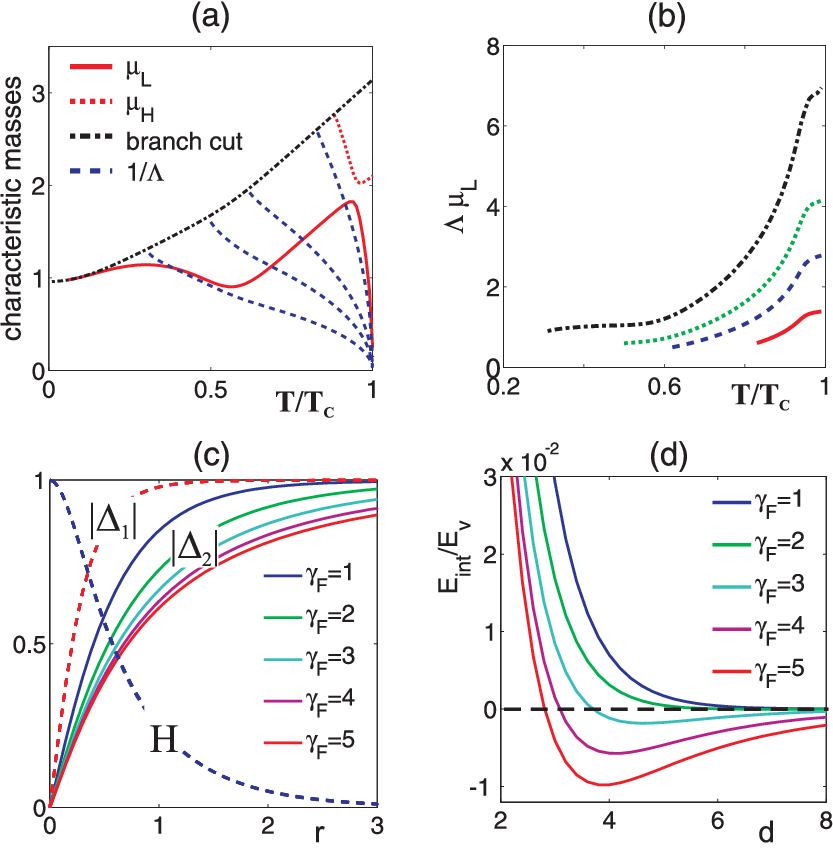
To demonstrate the type-1.5 behavior we have chosen the parameters in the self-consistency equation for the current such that the characteristic magnetic field localization length is much larger than . This leads to a existence of regular vortex lattices in a wide range of strong magnetic fields (i.e. when vortices are closely packed and thus experience only strong short-range repulsive interaction). However, the high magnetic field behavior notwithstanding, the vortex structures shown in Fig.3(c) clearly shows that i.e. the long-range interaction is attractive and thus the system in fact belongs to the type-1.5 regime.
Next, to demonstrate the type-1.5 superconductivity i.e. large-scale attraction and small-scale repulsion of vortices which originates from disparity of the variations of two gaps, we explicitly calculate the intervortex interaction energy. We evaluate the two-band generalization of the Eilenberger expression for the free energy of the two vortices positioned at the points and in plane. Here we generalize to two-band theory the method developed for calculation of asymptotic vortex interaction in singe-component theories [18]. The method assumes that for large separations, in the region the fields , and correspond to the single vortex placed at the point weakly perturbed by the presence of the second vortex. The interaction energy can be expressed through the integral over the line passing in the middle between vortices where
| (12) | ||||
The detailed derivation of the above expression can be found in the AppendixB. The indices correspond to the solutions of Eilenberger Eqs.(1) for isolated vortices positioned at the points . The first term in the Eq.(12) contains the magnetic field and the axial component of superfluid velocity distribution corresponding to the isolated vortex placed at the point .
In Fig.3(d) the interaction energy is shown as a function of the distance between two vortices . The energy is normalized to the single vortex energy . The plots on Fig.3(d) clearly demonstrate the emergence of type-1.5 behavior when the parameter is increased. This is manifested in the appearance non-monotonic behaviour of .
IV Low temperature vortex asymptotics and intrinsic proximity effect.
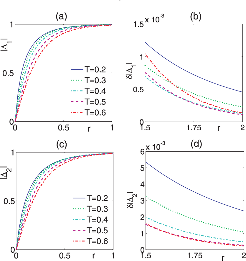
Finally we discuss the two-band superconductor with at . Note that qualitatively similar regime is realized in the two-band superconductor [15]. To model such situation we choose the coupling constants , and consider various values of . The temperature dependencies of the mass for different values of are shown in the Fig.1(d). Note that in this case, decreasing of intraband coupling leads to the decreasing of the at low temperatures. This anomalous behaviour of the characteristic length scale is clearly manifested in the vortex structure shown in Fig.(4). The near-core gap function profiles [Fig.4(a,c)] feature shrinkage of the vortex core at decreasing temperature, similarly to clean single-band superconductors[19]. However the asymptotics of gap functions [Fig.4(b,d)] are drastically different from the single-band case. Indeed, it can be seen that in a certain temperature domain the lower the temperature, the slower is the recovery the gap functions at large distances from the core. Such behavior in the two-band system is clearly in a sharp contrast with the overall vortex core shrinking with decreasing temperature in clean single-band superconductors.
Note that in the above case, at low temperatures we have . For the especially interesting regime of purely interband proximity effect-induced superconductivity in the weak band we can consider the limit . Then , where is the coherence length in a pure normal metal [2] describing the penetration length of superconducting correlations induced by the proximity effect in superconductor/normal metal (SN) hybrid structures[20]. Thus we obtain that the intrinsic proximity effect due to the interband coupling[11] can in certain cases be described by the similar length scale as the usual one in SN hybrid structures. At the temperature interval the mass grows linearly with temperature [Fig.1(d)].
V Conclusion
In conclusion, the rapidly growing family of discovered multiband superconductors (, Iron pnictides etc) requires understanding and classification of possible magnetic response of systems with multiple superconducting gaps. Here we reported a microscopic theory of magnetic response of a superconductor with two bands (the developed approach can be generalized to the case of a higher number of bands). We have shown that new physics which arises in multiband systems is the existence of several mixed gaps modes. This, in a range of parameters results in the existence of the type-1.5 superconducting regime. We described the system properties and emergence of type-1.5 regimes in the entire temperature regimes, in particular beyond the validity of a two-component GL theory. The universal feature of all the regimes supporting type-1.5 behavior is the thermodynamic stability of vortex excitations in spite of the existence of a mode which varies at a fundamental length scale larger than the magnetic field penetration length. It results in non-monotonic vortex interaction and appearance of the additional Semi-Meissner phase in low magnetic fields which is a macroscopic phase separation into (i) domains of two-component vortex state and (ii) vortex clusters where one of the components is suppressed.
VI Acknowledgments
The work is supported by the NSF CAREER Award No. DMR-0955902, the Knut and Alice Wallenberg Foundation through the Royal Swedish Academy of Sciences and by the Swedish Research Council, “Dynasty” Foundation, Presidential RSS Council (Grant No. MK-4211.2011.2) and Russian Foundation for Basic Research.
Appendix A Asymptotical behaviour of the gap functions.
We focus on the structure of the isolated axially symmetric vortex in two-band superconductor characterized by the non-trivial phase winding of the gap functions:
| (13) |
We begin by considering the asymptotical behaviour of the gap functions at distances far from the vortex core when the deviations of all fields from the homogeneous values are small. In this case the Eilenderger Eqs.(1) can be linearized in order to find the asymptotical behavior of the gap functions modules . To compare with the different linearlization problem in single-band case see Ref.(21).
To determine the asymptotic behaviour we use the transformation , and rewrite the Eilenberger Eqs.(1) in terms of the deviations from the vacuum state values and , . Then keeping the first order terms and in the l.h.s. we can rewrite the Eilenberger Eqs. in the following form (we omit the band index for brevity):
| (14) | ||||
where the higher order terms in , and are incorporated in the r.h.s. functions . In Eqs.(14) we introduce and the functions and . The higher order terms are incorporated in the functions .
Then we take the real part of the Eqs.(14) to obtain the following system
| (15) | ||||
Here omit the band index for brevity and denote . Below we will find the asymptotic of the gap fields treating the nonlinear terms in the r.h.s. of Eqs.(15) as source functions.
The solution of Eqs.(15) can be found in the momentum representation . Then we get
| (16) |
where the last term incorporates the higher order corrections:
| (17) |
After substituting it to the self-consistency Eq.(2) we get the expression for the order parameter
| (18) |
where
| (19) |
and the elements of the matrix are defined by and , where
| (20) |
The integrals entering the expressions (20) above are
so that
| (21) |
The source functions come from the nonlinear terms in Eilenberger Eqs.(15).
The Eq.(18) is the two-band response function. To compare with the single-band response function see [17]. In general the real space asymptotic behaviour of the order parameter (18) is determined by the contributions of the singularities of the response function which are poles and branch points at . Analogously to the consideration in Ref.(17) we assume the branch cuts to lie along the imaginary axis from to . The poles are determined by the zeros of the determinant , so that
Since we are interested in the asymptotic behaviour of the order parameter, we need only to take into account the poles of lying in the upper complex half plane below all the branch cuts. In this case all the zeros of the function are purely imaginary . Each of them can be associated with the particular mass of the gap function field which determine the characteristic length scale of the gap function variation. On the other hand the contribution from the branch cut contains all the length scales which are larger than the threshold one given by position of the lowest branch point where
| (22) |
Appendix B Energy of interaction between two vortices
B.1 General free energy expression
The two-band generalization of the Eilenberger expression for the free energy[22] reads as follows
| (23) | ||||
where
and
with
| (24) | ||||
where and
Then the variation of the free energy (23) with respect to the fields and gives the self-consistency Eqs.(4) and (2) correspondingly. The variation over and with the normalization condition taken into account yields the Eilenberger Eqs.(1). Provided the functions satisfy the Eqs.(1) the expression (24) can be rewritten as
| (25) |
B.2 Linearized theory of vortex interaction
To calculate the energy of vortex interaction we evaluate the free energy expression for the system of two vortices positioned at the points and in plane. Here we employ the method similar to that in [18].
Let us consider the half-plane containing only one of the vortices. We decompose the gap function into amplitude and phase (we omit the band index for brevity)
| (26) |
The total phase can be written in the following form , where
are the vortex phases and is a regular part of the phase. At the region we can make the gauge transformation removing the phase , since it does not contain singularities. After this transformation we can assume that the fields , and correspond to the solutions for a single vortex placed at the point weakly perturbed by the presence of the second vortex.
where we have introduced the superfluid velocity induced by the second vortex . Then we obtain
| (27) | |||
where
The last two terms in Eq.(27) can be rewritten as follows
| (28) | ||||
The first term in this expression cancels with the second and forth terms in Eq.(27). For the variation of magnetic field energy in Eq.(23) we obtain
Then we are left with the non-zero terms
| (29) | ||||
The energy of vortex interaction is . It can be expressed through the integral over the line so that
| (30) | ||||
To evaluate the second term in Eq.(30) it is convenient to bring the Eqs.(1) to the gauge invariant form[23] decomposing the gap functions into amplitude and phase (26) and transforming the Green’s functions as , . Then at the line we can put
where . Also we denote , [ stand for left (right) vortices]. Therefore up to the second order terms we obtain
| (31) | ||||
Now we use the symmetry relations and . Then the contribution to the interaction energy (30) from the first order term in Eq.(31) cancels with the analogous contribution from the left vortex. Also from the symmetry relations we obtain
| (32) | ||||
On the other hand
Therefore we get for the interaction energy
where
| (33) | ||||
and .
References
- [1] V.L. Ginzburg and L.D. Landau, Zh. Eksp. Teor. Fiz. 20, 1064 (1950); Landau, L.D. Collected Papers (Oxford: Pergamon Press, 1965) p. 546.
- [2] P.G. de Gennes, Superconductivity of metals and alloys (New York: Addison-Wesley, 1989).
- [3] A. A. Abrikosov, Sov. Phys. JETP, 5 1174 (1957) [Zh. Eksp. Teor. Fiz. 32 1442 (1957)]
- [4] U. Klein, Journal of Low Temp. Phys., 69 1 (1987).
- [5] A.E. Jacobs, Journal of Low Temp. Phys., 10, 137 (1973).
- [6] E. Babaev, J.M. Speight, Phys. Rev. B, 72 180502 (2005).
- [7] E. Babaev, A. Sudbø, N.W. Ashcroft, Nature 431, 666 (2004).
- [8] E. Babaev, Phys. Rev. Lett. 89, 067001 (2002).
- [9] V.V. Moshchalkov, V. H. Dao, L.F. Chibotaru, N.D. Zhigadlo, J. Karpinski, Phys. Rev. Lett. 102, 117001 (2009).
- [10] E. Babaev, J. Carlstrom, M. Speight, Phys. Rev. Lett., 105 067003 (2010).
- [11] J. Carlstrom, E. Babaev, M. Speight, Phys. Rev. B 83 174509 (2011)
- [12] J. Carlstrom, J. Garaud, E. Babaev, arXiv:1101.4599.
- [13] H. Suhl, B.T. Matthias, L.R. Walker, Phys. Rev. Lett. 3, 552 (1959).
- [14] T. Nishio, V.H. Dao, Q. Chen, L.F. Chibotaru, K. Kadowaki, V.V. Moshchalkov, Phys. Rev. B, 81, 020506(R) (2010).
- [15] A. Gurevich, Physica C, 456 160 (2007).
- [16] K. Tanaka, M. Eschrig, D.F. Agterberg, Phys. Rev. B 75, 214512 (2007).
- [17] M.C. Leung, A.E. Jacobs, Journal of Low Temp. Phys. 11 395, (1973).
- [18] L. Kramer, Phys.Rev. B, 3, 3821 (1971).
- [19] W. Pesch and L. Kramer, Journal of Low Temp. Phys. 15, 367 (1973);
- [20] G.Deutscher, P.G. de Gennes in Superconductivity ed. by R.D. Parcs, Vol.2, P.1005 (Marcel Dekker Inc., New York 1969)
- [21] G. Eilenberger, H. Buttner, Z. Physik 224, 335 (1969).
- [22] G. Eilenberger, Z. Phys., 214, 195 (1968).
- [23] T. Dahm, S. Graser, C. Iniotakis, N. Schopohl, Phys. Rev. B, 66, 144515 (2002).