Two photon decay of $Z^{\prime}$ as a probe of Bose symmetry violation at the CERN LHC

For all known particles, there is a remarkable one-to-one correspondence between their spin type and statistics type:

In quantum field theory, this spin-statistics connection (SSC) can be understood in different ways. For free fields, the connection was established using conventional lagrangian and group-theoretical methods [1].

Interacting fields were tackled using axiomatic quantum field theory (without any lagrangians), and by early 1960s the celebrated spin-statistics theorem was proved [2].

It is worth recalling that the axiomatic treatment of the spin-statistics connection [2] does not cover the case of quantum electrodynamics and other gauge theories including the Standard Model (for a detailed explanation, see [3], Sec. 8.1).

The physical root of this difficulty is the fact that while the photon is a massless spin-1 particle with only two polarizations, the corresponding 4-potential $A_{\mu}$ has four components.

Consequently, ordinary Hilbert space with positive metric cannot accomodate the 4-component field operator $A_{\mu}$, and the introduction of indefinite-metric space is required.

This is at odds with the axiom underlying the proof of the spin-statistics theorem, which states that the Hilbert space metric must be positive.

As a result, the original set of axioms [2] needs to be modified to include Hilbert spaces with indefinite metric as well. Although progress has been achieved in this area (see, e.g., [3], Ch.10) the extension of the spin-statistics theorem to gauge theories is yet to be formulated.

In any case, the theorem does not forbid small violation of the SSC and the question whether it exists or not remains open. (That does not mean, however, that construction of a theory with small statistics violation is easy. To date, most attempts to find a local relativistic quantum field theory with small statistics violation have been unsuccessful.)

There have been several works that have attempted to improve the original spin-statistics theorem by going beyond the Bose-Fermi alternative [4], and, in particular, to rule out the small violation of SSC. However, they also assume positivity of Hilbert space metric and hence do not apply to gauge theories.

Even if the small SSC violation was shown to be theoretically forbidden on the basis of general principles of QFT such as Lorentz invariance, locality etc., the experimental tests of SSC would still be of interest because they would be important tests of those general principles.

We may assume that at some extremal or small enough distances where the usual notions of the local fields become invalid, their proper reconsideration and a generalisation should be required, which can bring us the possibility of changing or correcting the usual Spin-Statistics Correspondence.

Since 1987 there have been significant theoretical and experimental efforts to motivate and find tiny departure from the established connection between spin and statistics.

Originally, most efforts [5-30], especially in the experimental field, were actually concentrated on discussing small violation of the Pauli exclusion principle rather than violation of Bose statistics. Many dedicated experiments have been performed to give strong bounds on the violation of the Pauli principle. Also, the topic was discussed in the context of string theories [31] and cosmology [32]. For recent reviews, see [33].

Later, Bose statistics came under scrutiny as well. Initially, experimental proposals of searching for deviations from Bose symmetry used the spin-zero nucleus of oxygen ${}^{16}O$ as the test object [34, 35].

For a review of subsequent experiments with $O_{2}$ and $CO_{2}$ molecules, see [36].

The first experimental upper limit on the validity of Bose statistics for photons was obtained in Ref. [37] based on the idea of forbidden two-photon decays of Z-boson.

The same idea was later explored in Ref. [38], in the context of low-energy, high-sensitivity atomic two-photon transitions (see also [39]).

This approach exploits one of the important consequences of the Bose symmetry, first observed by Landau [40] and Yang [41]: a pair of photons cannot form a state with total angular momentum equal to unity. The Landau-Yang theorem uses general principles of rotation invariance, gauge invariance, and Bose statistics to derive certain selection rules for decays of a parent particle into two photons. For a parent with spin one, the decay amplitude into the exchange-symmetric state of two photons vanishes.

Therefore, the decay of any spin-1 boson into two photons is absolutely forbidden (for a textbook proof, see, e.g., [42]). If, however photons do not obey Bose statistics, there will be a nonzero decay amplitude involving two photons in an exchange-antisymmetric state [37]. This provides a clear reason why the diphoton system is especially interesting in testing the degree with which Bose symmetry is exact.

Recent experiments have explored the possibility of small violations of the usual relationship between spin and statistics, which are impossible within conventional quantum field theory. Experiments searching for the transitions between atomic states with $J=0$ and $J^{\prime}=1$ for degenerate photons (i.e. photons of equal energies) test the Bose statistics at the eV scale and yield upper limit on the ratio $\nu$ of the rate of statistics-violating transitions to an equivalent statistics-allowed transition rate, $\nu<4.0\times 10^{-11}$ at the 90% confidence level [43]. At higher energies the limits on the branching fraction of two-photon decays of the triplet positronium (orthopositronium) $Br(oPs\to\gamma\gamma)\lesssim 2.4\times 10^{-5}$ [44] and charmonium $Br(\chi_{c1}\to\gamma\gamma)\lesssim 3.5\times 10^{-5}$ [45] have been reported. At the energy scale of 100 GeV the results of the search for the gauge boson $Z$ into two photons were obtained at LEP [46] $Br(Z\to\gamma\gamma)<1.4\times 10^{-4}$.

From general arguments, one can expect that any violations of Bose symmetry, if any, would be better manifested at higher energy scales. Then the question arises: could interesting physics be found by combining the idea of searching for Bose statistics violation and assumption that Bose symmetry might be broken at a high energy frontier at the CERN LHC? Out of all (neutral) spin 1 bosons it is natural to concentrate on the heaviest one- the new heavy gauge boson $Z^{\prime}$ which appears naturally in many extensions of the SM.

The explicit goal of this paper is to extend the results of the previos work [37] to the TeV scale and to show that the search for the decay $Z^{\prime}\to\gamma\gamma$ at the CERN LHC could result in a more radical departure from standard physics: the possible observation of a small violation of Bose statistics, which would provide strong evidence for the existence of new physics. The rest of the paper is organized as follows: in Sect.II we describe the phenomenological model [37] of the Bose symmetry violation and its extensions; we then show how the parameters of the model are constrained by theoretical arguments and electroweak precision data. Following this, Sec. III deals with the $Z^{\prime}$ sector in some detail. The main characteristics of the $Z^{\prime}$ boson are described within the framework of several $Z^{\prime}$ models. Section IV-VI present the results of a sensitivity study for the Bose symmetry violating process $pp\to Z^{\prime}\to\gamma\gamma$ at the CERN LHC at $\sqrt{s}=14$ TeV. Finally, Sec. VII presents the conclusions of this work.

In this section we describe a simple model of Bose symmetry violation suggested in Ref. [37] and its extensions.

The method [37] is to write down the most general form of the decay amplitude of the spin-1 particle into two photons and then apply the conditions of gauge invariance and Bose symmetry to that amplitude. If both conditions are applied, the resulting amplitude is exactly zero. However, if we impose the condition of gauge invariance but do not require the Bose symmetry, the resulting amplitude is not zero. We then can obtain the two-gamma decay rate of Z-boson and compare it to the experimentally known upper bound on the branching ratio of $Z\to\gamma\gamma$. In this way a direct bound on Bose symmetry violation for photons can be obtained [37].

Now, a few remarks about the relation of this method to alternative models of small Bose symmetry violation. The most well-studied model is ”the quon model” proposed in [47]. Quons are particles described by the commutation relations of the form:

However, it was shown in Ref.[48] that in relativistic field theories quons must be either fermions or bosons. For this reason, the quon theory cannot be used for the analysis of the decay $Z\to\gamma\gamma$.

Let us turn now to the construction of $Z\to\gamma\gamma$ decay amplitude. We require that this amplitude satisfies all the standard conditions, such as relativistic invariance and gauge invariance, but we do not require this amplitude to be symmetric under the exchange of photon ends. The most general Lorentz invariant form of the amplitude $S$ of the decay $Z\to\gamma\gamma$ is:

where $k_{1}$ and $k_{2}$ are photon momenta, $\epsilon_{1}$ and $\epsilon_{2}$ are photon polarization vectors, $\epsilon_{0}$ is $Z$-boson polarization vector.

Even though violation of SSC could require violation of Lorentz invariance as well, using more general parametrization in Eq. (4) would be overkill.

Note that terms in $c_{\lambda\mu\nu}$ proportional to $k_{1\mu},k_{2\nu}$ and $k_{1\lambda}+k_{2\lambda}$ do not contribute to $S$ due to the conditions

and can therefore be ignored.

We focus first on the part of $c_{\lambda\mu\nu}$ that does not contain the $\epsilon$-tensor: it has the following Lorentz invariant form:

Now, the condition of the electromagnetic gauge invariance reads

These conditions can be satisfied if we put

Then the amplitude $c_{\lambda\mu\nu}$ becomes [37]

In principle, $g$ could depend on some scalar products of the momenta, but in our case, since all the particles are on mass shell, we have $k_{1}k_{2}=M_{Z}^{2}/2$ (and, of course, $k_{1}^{2}=k_{2}^{2}=0$), so that $g$ is a pure number. Note that the above amplitude automatically satisfies the condition $(k_{1}+k_{2})^{\lambda}c_{\lambda\mu\nu}=0$. We see that this amplitude, as expected, violates Bose symmetry because

whereas Bose symmetry requires $c_{\lambda\mu\nu}(k_{1},k_{2})=+c_{\lambda\nu\mu}(k_{2},k_{1})$.

Thus the parameter $g$ can be interpreted as the parameter of Bose statistics violation which will be marked by the subscript $B1$: $g\equiv g_{B1}$.

Next, it can be shown that the following Lorentz-invariant terms containing the $\epsilon$-tensor also satisfy the conditions of gauge invariance and Bose-antisymmetry:

and

Now, calculating the width of the decay $Z\to\gamma\gamma$ with the help of the amplitude Eq.(9) we obtain ¹¹ 1 the difference between the numerical factors here and in Ref.[37] is due to a mistake in the latter.:

Experimentally, it has recently been measured at LEP [49] that

Therefore

Thus, taking into account that $\Gamma_{tot}(Z)\simeq 2.5$ GeV [49], finally, we can obtain our upper bound on the Bose violating coupling

We see that in the framework of this model the rate of the decay $Z\to\gamma\gamma$ is small; however, it can be enhanced for higher-mass particles. Hence, the heavier spin-1 $Z^{\prime}$ is a good candidate for the searching for effect of Bose symmetry violation through the $Z^{\prime}$ decay into two gammas.

A similar analysis can be carried out for the amplitudes of Eq.(11) and (12). The decay widths due to the amplitudes (11,12) are equal to:

The corresponding upper bounds on the constants $g_{B2},\;g_{B3}$ are:

In the context of our approach, the reason for treating the three amplitudes separately is purely technical and does not involve the essential physics. Indeed, adding the three amplitudes with three arbitrary coupling constants would be possible but it would only add considerable complexity and obscurity into experimental simulations without any gains in physical understanding.

A few remarks are now in order concerning the relationship between the approaches developed in Ref. [37] and a later work, Ref. [38].

In Ref. [38] it was claimed that the limit obtained in [37] is too weak to be of any significance. This conclusion was reached within a very specific model for Bose symmetry violation which is different from the model-independent approach suggested in [37]. A detailed discussion of similarities and differences between the two frameworks would be out of place in the present paper, so we restrict ourselves to a few general comments only.

In a nutshell, the difference is this: Instead of constructing the most general Bose-violating amplitude of the decay and the coupling constant $g_{B}$, the authors of Ref.[38] introduce the “probability for two photons to be in an antisymmetric state” $\nu$. The physical decay width $\Gamma$ is then obtained as $\Gamma=\Gamma_{B}+\nu\Gamma_{F}$, where $\Gamma_{B}$ is the width for the decay into ordinary “bose-photons”, and $\Gamma_{F}$ is the width of Bose-symmetry violating decay into “fermi-photons”. For instance, if the decay amplitude for the usual, “bose-photons” 1 and 2 is $A_{B}=A_{12}+A_{21}$, then the corresponding amplitude for “fermi-photons” would be $A_{F}=A_{12}-A_{21}$, with $\Gamma_{B}\propto|A_{B}|^{2}$ and $\Gamma_{F}\propto|A_{F}|^{2}$.

This approach may look simple and natural, but five points should be kept in mind:

1. Well-known difficulties arise when $\nu$ is introduced. According to quantum mechanics, every probability is the square of (modulus of ) amplitude. So, after we introduced $\nu$ we must introduce the “amplitude for two photons to be in an antisymmetric state”, let us call it $\mu$.

So, the Bose-violating two-photon state will be $|B\rangle=N(|S\rangle+\mu|A\rangle)$ ($N$ is the normalization factor). Next, due to superposition principle, we can add to it the state $-N|S\rangle$, obtaining $|B^{\prime}\rangle=N\mu|A\rangle$. Now, $|B^{\prime}\rangle$ is obviously not properly normalized, and after normalization, it becomes just $|B^{\prime\prime}\rangle=|A\rangle$, i.e. “amplitude for two photons to be in an antisymmetric state” becomes 1 instead of $\mu$.

So it is hard to give physical meaning to the concept of “probability for two photons to be in an antisymmetric state”, unless superposition principle is modified in some way.

2. It is believed [38] that the ‘Bose’ and ‘Fermi’ amplitudes $A_{B}$ and $A_{F}$ do not interfere, i.e., the total probability is assumed to be $\Gamma\propto|A_{B}|^{2}+\nu|A_{F}|^{2}$ rather than $\Gamma\propto|A_{B}+\mu A_{F}|^{2}$. In Ref. [38] this assumption is justified by invoking the rule that the matrix elements of a symmetric Hamiltonian has zero matrix elements between the states of different symmetry [7]. However, this rule appears to be superfluous as the model [38] itself dictates whether $A_{B}$ and $A_{F}$ interfere or not. Indeed, in this model, the necessary and sufficient condition of non-interference is $|A_{12}|=|A_{21}|$ (assuming for simplicity that $\mu$ is real). (It should be noted that whether the superposition is coherent or incoherent is irrelevant for the decay $Z^{\prime}\rightarrow\gamma\gamma$, which is forbidden at zeroth order.)

3. Should we consider $\nu$ is a ‘universal’ parameter, i.e., independent of the physical process, energy scale etc.? This may or may not be true depending on the details of the underlying specific theory. For instance, it is not inconceivable that $\nu$ could be energy-dependent and grow with energy. In this case, upper limits on $\nu$ obtained in low- and high-energy processes would not be directly comparable to each other.

4. Finally, Ref.[38] makes (implicitly) a strong but arbitrary conjecture that the amplitude $A_{12}$ should be calculated in the Standard Model. There is nothing wrong with it as long as we remember that:
—this is just one of many possible assumptions, and certainly not the most general or unique.
—the parameter $\nu$ is meaningful only if this assumption is made.

5. If we pursued a similar approach, the result would be that the rate of $Z^{\prime}\rightarrow\gamma\gamma$ decay becomes rather small: due to a fermion loop it would be suppressed by at least a factor of $\alpha^{2}$ (cf. [38]). As a result, its search at LHC would require a higher sensitivity.

By contrast, Ref. [37] did not rely on this or similar conjectures, but tried to be more general. In this general approach, there is no point in estimating $\nu$, because this parameter belongs to a different model based on additional specific assumptions.

We feel that at the moment our level of understanding is, unfortunately, insufficient for telling on purely theoretical grounds which approach is correct, and we need an experimental search that could settle the issue.

Consider now the new boson $Z^{\prime}$, which appears in many models of physics beyond the SM, see e.g. [50]-[58]. The $Z^{\prime}$ is assumed to be a more massive than the gauge boson $Z$ of the standard model. The most direct channel to probe the existence of the $Z^{\prime}$ at a hadron collider, such as the CERN LHC [59], is the Drell-Yan process. The $Z^{\prime}$ that decay to leptons, $pp\to Z^{\prime}\to l^{+}l^{-}+X$ with $l=e,\mu$, have a simple, clean experimental signature, and potentially could be discovered at the LHC with a mass up to 5 TeV, see e.g.[60, 61]. This new object is supposed to be neutral, colorless and self-adjoint, i.e., it is its own antiparticle. The mass of the new boson could be identified unambiguously by a study of a resonance peak in the dilepton invariant mass distribution. The $Z^{\prime}$ may be classified according to its spin, which could be defined by measuring the dilepton angular distribution in the reconstructed $Z^{\prime}$ rest frame. The $Z^{\prime}$ could be a spin-0 $\overline{\nu}$ in R-parity violating SUSY, a spin-2 Kaluza-Klein (KK) excitation of the graviton as in the Randall-Sundrum (RS) model, or even a spin-1 KK excitation of a SM gauge boson from some extra dimensional model [53]. Another possibility for the spin-1 case is that the $Z^{\prime}$ is a true $Z^{\prime}$, i.e. a new neutral gauge boson, which is the carrier of a new force, arising from an extension of the SM gauge group. For much more extensive discussions of specific models and other implications see several excellent reviews [52, 53, 54, 62, 57], and a more complete list of references therein.

The current best direct experimental lower limits on the mass of $Z^{\prime}$ of a few popular models came from the Tevatron and restrict the $Z^{\prime}$ mass to be greater than about 900 GeV when its couplings to SM fermions are identical to those of the Z boson [49].

Consider now the allowed branching fraction $Br(Z^{\prime}\to\gamma\gamma)=\Gamma(Z^{\prime}\to\gamma\gamma)/\Gamma(Z^{\prime}\to l^{+}l^{-})$ in several interesting $Z^{\prime}$ models. First, we shortly describe these models and the SM fermions couplings the $Z^{\prime}$.

• •

  the E₆ models are described by the breaking chain $E_{6}\to SO(10)\times U(1)_{\psi}\to SU(5)\times U(1)_{\chi}\times U(1)_{\psi}\to SM\times U(1)_{\beta}$. Many studies of $Z^{\prime}$ are focusing on the two extra $U(1)^{\prime}$ which occur in the above decomposition of the $E_{6}$. The lightest $Z^{\prime}$ is defined as :

  $$Z^{\prime}=Z^{\prime}_{\chi}cos\beta+Z^{\prime}_{\psi}sin\beta$$

  (19)

  where the values $\beta=0$ and $\beta=\pi/2$ corresponds to pure $Z^{\prime}_{\chi}$ and $Z^{\prime}_{\psi}$ states of the $\chi$- and $\psi$-model, respectively. The value $\beta=arctan(-\sqrt{5/3})$ is related to a $Z^{\prime}_{\eta}$ boson that would originate from the direct breaking of $E_{6}$ to a rank-5 group in superstrings inspired models.

• •

  the Left-Right Symmetric (LRSM) model is based on the symmetry group $SU_{C}(3)\otimes SU_{L}(2)\otimes SU_{R}(2)\otimes U(1)_{B-L}$ [63], in which $B$ and $L$ are the baryon and lepton numbers, respectively. The model necessarily incorporates three additional gauge bosons $W^{\pm}_{R}$ and $Z^{\prime}$. The most general $Z^{\prime}$ is coupled to a linear combination of right-handed and $B-L$ currents:

  $$J^{\mu}_{LR}=\alpha_{LR}J^{\mu}_{3R}-(1/2\alpha_{LR})J^{\mu}_{B-L}$$

  (20)

  where $\alpha_{LR}=\sqrt{(c_{W}^{2}g_{R}^{2})/s_{W}^{2}g_{L}^{2})-1}$, with $g_{L}=e/s_{W}$ and $g_{R}$ are the $SU(2)_{L}$ and $SU(2)_{R}$ coupling constant with $s_{W}^{2}=1-c_{W}^{2}=sin^{2}\Theta_{W}$. The $\alpha_{LR}$-parameter is restricted to be in the range $\sqrt{2/3}\lesssim\alpha_{LR}\lesssim\sqrt{2}$. The upper bound corresponds to the so-called manifest LRSM with $g_{l}=g_{R}$, while the lower bound corresponds to the $\chi$-model discussed above, since $SO(10)$ can results to both $SU(5)\times U(1)$ and $SU(2)_{R}\otimes SU(2)_{L}\otimes U(1)$ breaking parameter. To simplify our study, we will use further the following standard assumptions: (i) the mixing angles are small; (ii) right-handed CKM matrix is identical to the left-handed one, and (iii) $g_{R}=g_{L}$.

• •

  in the sequential model (SSM) the corresponding $Z^{\prime}$ boson has the same couplings to fermions as the $Z$ of the SM. The $Z^{\prime}$ could be considered as an excited state of the ordinary $Z$ in models with extra dimensions at the weak scale.

• •

  the Stueckelberg extension of the SM (StSM) is based on the gauge group $SU(3)_{C}\otimes SU(2)_{L}\otimes U(1)_{Y}\otimes U(1)_{X}$ [64]. This extension of the SM involves a mixing of the $U(1)_{Y}$ hypercharge gauge field and the $U(1)_{X}$ Stueckelberg gauge field. The Stueckelberg gauge field has no couplings to the visible sector fields, while it may couple to a hidden sector, and thus the new physical $Z^{\prime}$ gauge boson connects with the visible sector only via mixing with the gauge bosons of the physical sector. These mixings, however, must be small because of the LEP electroweak constraints and consequently the couplings of the $Z^{\prime}$ boson to the visible matter fields are extra weak, leading to a very narrow $Z^{\prime}$ resonance. The width of such a boson could be as low as a few MeV or even lower. An exploration of the Stueckelberg $Z^{\prime}$ boson in the Tevatron data was recently carried out in [65]. Such a resonance may also be detectable via the Drell-Yan process at the LHC by an analysis of a dilepton pair arising from the $Z^{\prime}$ decay [66]. The coupling structure of the Stueckelberg $Z^{\prime}$ gauge boson with visible matter fields is suppressed by small mass mixing parameters thus leading to a very narrow $Z^{\prime}$ resonance. Below we will assume that the $Z^{\prime}-Z$ mixing strength is $\epsilon=0.06$ [65].

The $Z^{\prime}$ boson partial decay width into a fermion-antifermion pair is given by

where $N_{C}$ is a color factor ($N_{C}=3$ for quarks and $N_{C}=1$ for leptons), $g^{f}_{L},g^{f}_{R}$ are the left- and right-handed couplings of the $Z^{\prime}$ to the SM fermions, $\alpha$ is the electromagnetic coupling constant, which is $\alpha\simeq 1/128$ at the $M_{Z^{\prime}}$ scale, and $\sqrt{\eta_{f}}(=m_{f}/m_{Z`})$ is assumed to be $\ll 1$. The left-handed couplings of the $Z^{\prime}$ to the SM neutrinos are $g^{f}_{L}=\frac{3cos\beta}{2\sqrt{6}}+\frac{\sqrt{10}sin\beta}{12}$ and $g^{f}_{L}=\frac{1}{2\alpha_{LR}}$ for E₆ and LRSM models, respectively, while the right-handed couplings $g^{f}_{R}=0$ in both models. The $(g^{f}_{L})^{2}$ is restricted to lie in the range $0.07(\beta\simeq\pi/2)\lesssim(g^{f}_{L})^{2}\lesssim 0.45~(\beta\simeq 0.4)$ for the E₆ model [67], and in the range $1/8\lesssim(g^{f}_{L})^{2}\lesssim 3/8$ for the LRSM model. The detail discussions of the StSM $Z^{\prime}$ decay modes and couplings can be found in [66].

For the decay rate $Z^{\prime}\to\gamma\gamma$ in the $Z^{\prime}$ mass range $M_{Z^{\prime}}\lesssim 5$ TeV one may expect

as it follows from Eqs.(13,16).

Due to the possible strong dependence of the couplings $g_{B}$ on the boson mass and the discussion at the end of Section II, the inequality (22) should be viewed as an indication of the ballpark of the possible values of the width, rather than the firm limit. The same applies to Fig.3 and caption to Table 1. In Table 1 expected properties of $Z^{\prime}$ bosons for several models are summarized. The $Z^{\prime}\to\gamma\gamma$ decay rate is calculated by taking into account the LEP limit on the Bose violation coupling (16).

Next, let us explain how to search for the $Z^{\prime}\to\gamma\gamma$ decay at the LHC. The $Z^{\prime}$ decay into two photons is a rare decay mode, with a branching fraction $B(Z^{\prime}\to\gamma\gamma)$ in the range of $\lesssim 10^{-4}-10^{-3}$. The final state consists of two high $p_{T}$ photons, $p_{T}\simeq M_{Z^{\prime}}/2$ , detected in a LHC electromagnetic calorimeter surrounding the $pp$ collision region [60, 61]. The experimental signature of the $Z^{\prime}\rightarrow\gamma\gamma$ decay is a peak in the invariant mass distribution of these photons over the continuum background. An important point is that if the decays of the $Z^{\prime}$ into leptons occur, the position of the $Z^{\prime}$ mass peak and its expected experimental width in the diphoton invariant mass distribution can be predicted by the analysis of on-peak data based on the observation of a leptonic $Z^{\prime}$ decay mode. The allowed maximal branching fraction $\Gamma(Z^{\prime}\to\gamma\gamma)/\Gamma(Z^{\prime}\to\mu^{+}\mu^{-})$ calculated for the Bose violating coupling constant $g_{B1}=1.0\times 10^{-2}$ taking into account (22) is shown in Table 1. One can see, that, for example, for the $g_{B}\simeq 10^{-2}$, the process $Z^{\prime}\to\gamma\gamma$ could amount to more then 1% of the total muonic $Z^{\prime}$ decay rate in the StSM model. Hence, if $Z^{\prime}$ is observed at the LHC the search for its diphoton decay mode is of great interest for possible observation of Bose symmetry violation.

For the appropriate $Z^{\prime}$ coupling constants discussed above, the production cross section $\sigma(pp\to Z^{\prime})\cdot B(Z^{\prime}\to\gamma\gamma)$ at the LHC for several $Z^{\prime}$ models are calculated in the framework of PYTHIA [68]. In this evaluation, the default CTEQ5L parton distribution functions [69] are used with no K-factors included. In most of our analysis we also neglect errors associated with imprecise knowledge of parton distribution functions; the related systematic errors, however, will be included into the final results: see Sec. VI. Fig.1 shows the production cross section $\sigma(pp\to Z^{\prime})\cdot B(Z^{\prime}\to\gamma\gamma)$ at the LHC at $\sqrt{s}=14$ TeV in the E₆, LRSM and Stückelberg models calculated as a function of the $Z^{\prime}$ mass assuming the value of the coupling constant $g_{B1}=1.0\times 10^{-2}$. The StSM curve is calculated for the $Z^{\prime}-Z$ mixing strength value $\epsilon=0.06$. Interestingly, although the StSM production cross section $\sigma(pp\to Z^{\prime})\cdot B(Z^{\prime}\to l^{+}l^{-})$ is an order of magnitude below those of other $Z^{\prime}$ models, the cross section $\sigma(pp\to Z^{\prime})\cdot B(Z^{\prime}\to\gamma\gamma)$ is comparable to the corresponding cross sections in other models.

Although the experimental signature of the decay $Z^{\prime}\to\gamma\gamma$ at the LHC is expected to be relatively clean, in order to discover this process one has to determine whether the $Z^{\prime}$ mass peak in the diphoton invariant mass spectrum could be distinguished from the background due to the standard model reactions. At a hadron collider experiment the diphoton production with a large invariant mass is a well known and studied background not only for the search of the two photon decay of the Higgs boson, but also for searches of new heavy resonances, extra spatial dimensions, or cascade decays of heavy new particles [60, 61] where it is a source of significant background. The dominant standard model background sources to our signal are (see e.g.[60]):

• •

  the prompt $\gamma\gamma$ production either form the quark annihilation or gluon fusion. As the final states from our signal and from these processes are identical, this is irreducible intrinsic background.

• •

  The $\gamma+$jets production consisting of two parts: (i) prompt photon from hard interaction plus the second photon coming from the outgoing quark due to initial and final state radiation and (ii) prompt photon from hard interaction plus the decay of a neutral hadron (mostly isolated) in a jet, which could fake a decay photon. The $\gamma+jet$, $pp\to\gamma+jet+X$ with a jet faking photon production turned out to be one of the most important backgrounds.

• •

  The background from QCD hadronic jets, consisting of quarks that fragment into a high momentum $\pi^{0}$ , which subsequently decays as $\pi^{0}\to\gamma\gamma$. The resulting photon showers may overlap, and can pass the photon selection.

• •

  other possible sources of background is the Drell Yan productions $pp\to e^{+}e^{-}+X$. The production of a high-transverse-momentum lepton pair, can lead to a diphoton final state if both electrons produce hard bremsstrahlung photons, or if the electron tracks fail to be properly reconstructed. We, however, assume a high efficiency of a LHC detector silicon tracker veto which, being applied to photon-containing candidate events, makes this background negligible.

To make quantitative estimates, we performed simplified simulations at the generator level of the $Z^{\prime}$ production followed by the decay $Z^{\prime}\to\gamma\gamma$ in the reaction $pp\to Z^{\prime}$ and the corresponding background processes at the LHC. We consider, as an example, the CMS detector [60]. As the signal events preferentially populate the large transverse momentum part of the phase space, events were generated with $P_{T}>100$ GeV (CKIN(3) parameter) and $|\eta|<2.7$ respectively. This allows us to reduce the time of computations and also to exclude of a very large fraction of the standard model events, which are peaked at small transverse momenta.

The CMS detector is described in detail in Ref. [60]. It consists of several subsystems: a superconducting magnet, a Si-tracker surrounded by an electromagnetic calorimeter followed by a hadronic calorimeter and muon chambers used for the detection and reconstruction of the events. The CMS experiment uses lead tungstate crystals for the electromagnetic calorimeter (ECAL). Each crystal measures about 22 $\times$ 22 mm² and covers $0.0175\times 0.0175$ (about $1^{o}$ ) in the $\Delta\eta-\Delta\phi$ space ($\phi$ being the azimuth angle).

For photon reconstruction at the generator level, we have used the “hybrid” clustering algorithm, to account for also fake photons arising from jets [70]. Photon candidates are reconstructed as superclusters in the CMS electromagnetic calorimeter (ECAL), within the fiducial regions of the barrel (EB) $|\eta|<1.4442$ and endcaps (EE) $1.566<|\eta|<2.5$. The superclusters are extended in $\phi$ to recover the energy deposited by electron bremsstrahlung and photon conversions. We consider a photon in the ECAL as a local deposition of electromagnetic energy by electrons or photons contained in a cone $R=\sqrt{\Delta\eta^{2}+\Delta\phi^{2}}<0.09$ with no associated tracks. This definition is equivalent to $10\times 10$ crystal size in the CMS detector. The CMS experiment uses $5\times 5$ crystal size to form an energy cluster to reconstruct a photon candidate. However, in our efforts to mimic this reconstruction process at the generator level, we choose to be conservative and use only a $10\times 10$ crystal. The momentum of the photon candidate is defined as the vector sum of the momenta of the electromagnetic objects in such a crystal.

As mentioned above, the main challenge to identifying the true photon candidates arises from jets faking photons, see e.g. [60]. This occurs when a jet from the standard model processes with $\gamma+jet$ or $jet-jet$ final state is dominated by a neutral hadron, such as, for example, a $\pi^{0}$ or $\eta$, which decays into two photons. If the hadron is highly energetic, so that the cosine of the opening angle between the two decay photons is $cos(\Theta_{\gamma_{1}\gamma_{2}})>0.9$, this angle is difficult to resolve and the photons can be misidentified as a single energetic photon. To suppress such backgrounds, we use various isolation variables, without, however, taking into account such photon object characteristics as the lateral and longitudinal electromagnetic shower shape. Jets typically have a larger number of charged particles reconstructed in their vicinty, and also a larger ratio of hadronic to electromagnetic deposited energy than photons. Likewise, hadronic and electromagnetic deposits arising from jets will be less isolated than for photons. Fake photon signals arising from a jet can be rejected by requiring either the absence of charged tracks above a certain minimum transverse momentum($P^{tr}_{Tmin}$ ) associated with the photon or the absence of additional energetic particles in an annular cone ($R_{iso}$) around the photon candidate. Following the diphoton analysis similar to Ref.[71], we have considered two variables for the isolation purposes: (i) the number of tracks ($N_{tr}$) from charged particles, such as $\pi,K,p,...$, inside a cone around the photon and (ii) the scalar sum of transverse energy ($E_{T}$) inside a cone around the photon. To identify the photons from the decay $Z^{\prime}\to\gamma\gamma$, the following $\gamma$ events selection criteria are used:

• •

  $P^{\gamma 1}_{T}\geq 100$ GeV, $P^{\gamma 2}_{T}\geq 100$ GeV;

• •

  $|\eta^{\gamma 1,\gamma 2}|<2.5$, $|\eta^{\gamma 1,\gamma 2}|\neq 1.4442-1.5666$;

• •

  $cos(\Theta_{\gamma 1,\gamma 2})\leq 0.9$;

• •

  $N_{tr}=0$ for $P^{tr}_{T}\geq 3.0$ GeV within $R_{iso}\leq 0.35$;

• •

  $E_{T}<5.0$ GeV within $R_{iso}\leq 0.35$;

Using this algorithm and requiring the photon to be isolated, the estimated probability of a jet faking a photon in $\gamma+jet$ channel is $\simeq 10^{-4}-10^{-3}$. The major sources of fake photons are $\pi^{0}$ ($\gtrsim 80\%$), with the rest coming from other sources.

As the next step, the signal event candidates are selected by requiring that the final state contain at least two or more isolated photons and a jet(s). Events are studied in which either both photons are in the barrel calorimeter, or one photon is in the barrel and the other is in the end cup calorimeter. The diphoton invariant mass distribution is calculated for two highest $P_{T}$ photons and histogrammed in bins equivalent to the mass resolution. The combined acceptance and selection efficiency for events with $P_{T}>100$ GeV and for $M_{Z}^{\prime}>1000$ GeV is found to be $\gtrsim 70\%$.

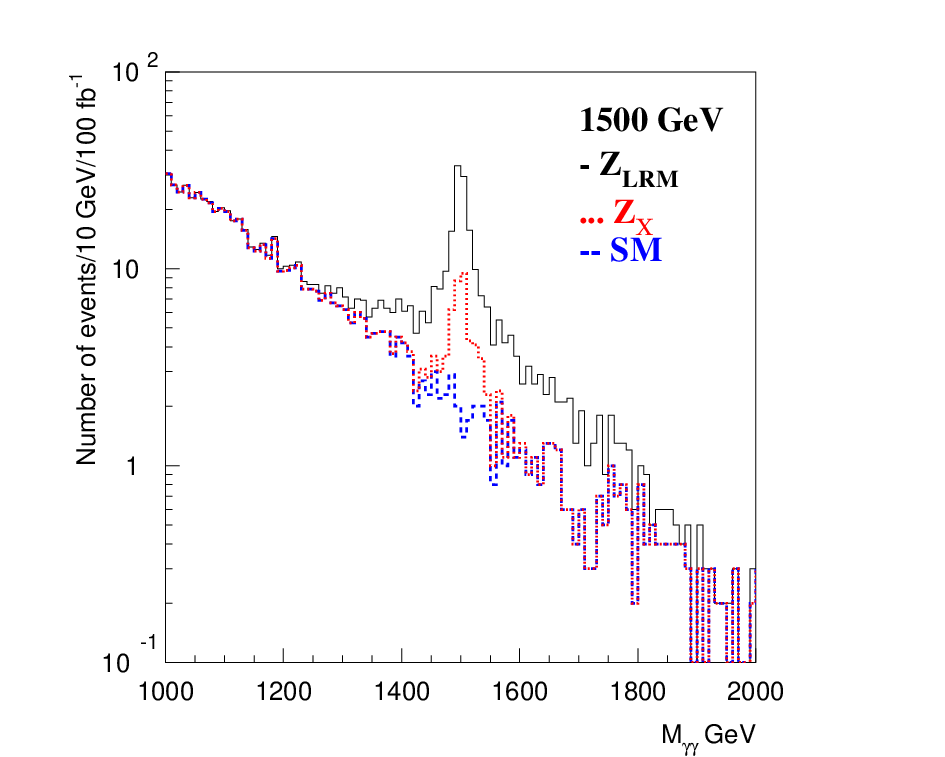
In Fig. 2 the invariant mass $M_{\gamma\gamma}$ distributions in the presence of the standard model background are shown for events simulated for the LRSM and E₆($Z_{\chi}$) models for the $Z^{\prime}$ with the mass of 1.5 TeV, the Bose violating coupling $g_{B1}=1.0\times 10^{-2}$, and the LHC integrated luminosity $L=150~fb^{-1}$. The additional broad peak and long tails below the $Z^{\prime}$ peak are from a combinatorial background due to the wrong choice of photons. For the invariant $\gamma\gamma$-mass $\gtrsim$ 1 TeV, the background under the $Z^{\prime}$ peak drops quickly.

The significance of the discovery of the $Z^{\prime}\to\gamma\gamma$ events can be estimated as [72]:

where $N_{S}$ and $N_{B}$ are the numbers of signal and background events respectively, which pass the selection criteria described above. These numbers of events are estimated from a search for the $Z^{\prime}\to\gamma\gamma$ mass peak, which was performed in the following way. For every $Z^{\prime}$ mass value, the region around it in the $M_{\gamma\gamma}$ distribution was fitted with a parametrized signal shape centered at the $M_{\gamma\gamma}$ value and superimposed over a polynomial background. The normalization of each component is allowed to float in the fit. This procedure is also used for the background estimate as a function of $M_{\gamma\gamma}$, with statistical uncertainties propagated from the fits. The systematic errors discussed below are also propagated to the fit procedure. The discovery potential of the $Z^{\prime}\to\gamma\gamma$ decay with the CMS detector is estimated assuming $S\gtrsim 3$.

The final results of this analysis are presented in Fig.3, where the most stingent limits for the coupling constant $g_{B}1$ obtained for the LRS model are shown as a function of $Z^{\prime}$ mass. For the total luminosity of 100 fb^-1 and the mass about 1 TeV, the limits are about one order of magnitude lower than the corresponding present limit from the search for $Z\to\gamma\gamma$ decay mode at LEP, thus making the process $Z^{\prime}\to\gamma\gamma$ feasible for observation at the LHC.

For the higher integrated luminosity of 1000 fb^-1, the use of $pp\to Z^{\prime}$ reaction allows to probe the decay $Z^{\prime}\to\gamma\gamma$ for the $Z^{\prime}$ masses up to 2 TeV.

The systematic errors in the number of expected $Z^{\prime}\to\gamma\gamma$ events coming from various background uncertainties are small since the background itself is rather small and the discovery region is usually limited by the fast drop of the signal cross section at high $Z^{\prime}$ mass. The largest systematic uncertainties of the expected number of $Z^{\prime}$-bosons arise from the luminosity measurement (6%) and the choice of PDF (5%). The latter uncertainty is determined from the variation in the efficiency when employing different PDF parameterizations. To study the effect of the detector energy resolution on this analysis, the energy of the photons was smeared with the stochastic term of the CMS electromagnetic calorimeter energy resolution [70]. Due to limitations in computing time, we did not fully simulate the background from jet-jet events. Although the dijet cross section is quite large, given the low probability of a jet faking a photon it is found that the kinematical and isolation cuts used above reject the dijet background substantially [71]. To get conservative estimate, we include uncertainties in the background estimate of 15%. Finally, the error of the measured LHC integrated luminosity is taken to be 3% [70].

To summarize, we consider a phenomenological model of the Bose statistics violation. We show that if a new heavy $Z^{\prime}$ boson is observed at LHC, further searches for the $Z^{\prime}\to\gamma\gamma$ decay mode would suggest an interesting additional direction to probe Bose symmetry violation at the high energy frontier. We have demonstrated that the discovery regions in the ($g_{B1};M_{\gamma\gamma}$) parameter space for the $Z^{\prime}\to\gamma\gamma$ decay substantially extend the excluded region from the CERN LEP. The low-energy experiment in atomic spectroscopy might be a sensitive probe of Bose symmetry violation that is complementary to collider experiments.