跳到论文正文
W Papers独立论文阅读器 arXiv:1102.5679 论文正文 计算阅读时间 · 0%
引用这篇论文根据当前论文元数据生成,正式投稿前建议核对。


License: arXiv.org perpetual non-exclusive license
arXiv:1102.5679v2 [hep-ph] 09 May 2011

March 2011

Higgs Mediated EDMs in the Next-to-MSSM :
An Application to Electroweak Baryogenesis

Kingman Cheunga,b,c, Tie-Jiun Houa,b, Jae Sik Leeb, and Eibun Senahab

a Department of Physics, National Tsing Hua University, Hsinchu, Taiwan 300
bPhysics Division, National Center for Theoretical Sciences, Hsinchu, Taiwan 300
cDivision of Quantum Phases & Devices, Konkuk University, Seoul 143-701, Korea

ABSTRACT

We perform a study on the predictions of electric-dipole moments (EDMs) of neutron, Mercury (Hg), Thallium (Tl), deuteron, and Radium (Ra) in the framework of next-to-minimal supersymmetric standard model (NMSSM) with CP-violating parameters in the superpotential and soft-supersymmetry-breaking sector. We confine to the case in which only the physical tree-level CP phase (ϕλ′−ϕκ′)(\phi^{\prime}_{\lambda}-\phi^{\prime}_{\kappa}), associated with the couplings of the singlet terms in the superpotential and with the vacuum-expectation-values (VEVs), takes on a nonzero value. We found that the one-loop contributions from neutralinos are mostly small while the two-loop Higgs-mediated contributions of the Barr-Zee (BZ) type diagrams dominate. We emphasize a scenario motivated by electroweak baryogenesis.

Keywords: Supersymmetry, Next-to-minimal supersymmetric standard model, CP violation, electric-dipole moments, Electroweak baryogenesis

1 Introduction

Supersymmetry (SUSY) is the leading candidate for the physics beyond the standard model (SM). It not only solves the gauge hierarchy problem, but also provides a dynamical mechanism for electroweak symmetry breaking and cosmological connections such as a natural candidate for the dark matter and baryogenesis. The minimal supersymmetric extension of the SM (MSSM) has attracted much phenomenological and theoretical interests but it suffers from the so-called little hierarchy problem and the μ\mu problem.

An extension with an extra singlet superfield, known as the next-to-minimal supersymmetric standard model (NMSSM) [1, 2, 3, 4, 5, 6] was motivated to provide a natural solution to the μ\mu problem. The μ\mu parameter in the term μ​Hu​Hd\mu H_{u}H_{d} of the superpotential of the MSSM naturally has its value at either MPlanckM_{\rm Planck} or zero (due to a symmetry). However, the radiative electroweak symmetry breaking conditions require the μ\mu parameter to be of the same order as the ZZ-boson mass for fine-tuning reasons. Such a conflict was coined as the μ\mu problem [7]. In the NMSSM, the μ\mu term is generated dynamically through the vacuum-expectation-value (VEV), vSv_{S}, of the scalar component of the additional gauge singlet Higgs superfield S^\widehat{S}, which is naturally of the order of the SUSY breaking scale. Thus, an effective μ\mu parameter of the order of the electroweak scale is generated. The NMSSM was recently revived because it was shown that it can effectively relieve the little hierarchy problem [8]. Due to the additional Higgs singlet field and an approximate PQ symmetry, the NMSSM naturally has a light pseudoscalar Higgs boson a1a_{1}. It has been shown [8] that, in most parameter space that is natural, the SM-like Higgs boson can decay into a pair of light pseudoscalar bosons with a branching ratio larger than 0.70.7. Thus, the branching ratio of the SM-like Higgs boson into b​b¯b\bar{b} would be less than 0.30.3 and so the LEPII bound is effectively reduced to around 100 GeV [9]. Since the major decay modes of the Higgs boson are no longer b​b¯b\bar{b}, unusual search modes have been investigated [10].

CP violation is one of the necessary ingredients for successful baryogenesis [11]. Although the SM can accommodate CP violation originating from the Cabibbo-Kobayashi-Maskawa matrix [12], it turns out that its effect is way too small to generate sufficient baryon asymmetry (∼10−10\sim 10^{-10}) [13] ** * Another shortcoming in the SM baryogenesis is that the electroweak phase transition is a smooth crossover for mh>m_{h}> 73 GeV [14], rendering thermal nonequilibrium unrealizable.. This fact suggests, in turn, that there should be an extra source of CP violation which has not been probed yet. CP violation relevant to electroweak baryogenesis (EWBG) [15] by construction must appear in the Higgs self interactions and/or the Higgs interactions with the other particles whose masses are 𝒪⁡(100)\mathcal{O}(100) GeV. Therefore, such CP violating effects can be communicated to the low energy observables which are measurable in the near future experiments. A lot of effort on the EWBG study have been made in the new physics models such as the MSSM [16], the two-Higgs doublet model [17] and the singlet-extended MSSM [18, 19].

The MSSM offers many possible sources of CP violation beyond the single Kobayashi-Maskawa phase in the SM. As far as the Higgs sector is concerned, the non-vanishing CP phases could induce significant mixing between the CP-even and CP-odd states radiatively [20, 21, 22, 23], giving rise to a number of interesting CP violating phenomena and substantial modifications to Higgs-boson phenomenology [24, 25]. In particular, the lightest Higgs boson can be as light as a few GeV with almost vanishing couplings to the weak gauge bosons when the CP-violating phases are maximal. The decay patterns of the heavier Higgs bosons become much more complicated compared to the CP-conserving case because of the loss of its CP parities [26, 27]. These combined features make the Higgs boson searches at LEP difficult, consequently, the Higgs boson lighter than ∼\sim 50 GeV can survive the LEP limit [28].

The non-observation of electric dipole moments (EDMs) for Thallium [29], neutron [30], and Mercury [31, 32] is known to constrain the CP-violating phases very tightly. It is generally believed that one-loop contributions dominate and we set the phases to 𝒪⁡(0){\cal O}(0) to make the null results of the EDM searches consistent within most of the parameter space †† † Nevertheless, accidental cancellations among various contributions may occur in the three measured EDMs, thus still allowing sizable CP phases even with the SUSY particles lighter than 𝒪⁡(1​TeV){\cal O}(1~{\rm TeV}) [33, 34].. However, we point out in this work that it may not be the case in the framework of NMSSM with CP-violating parameters. Even if we set the CP phases of the parameters appearing in the MSSM to zero, there could be potentially large nontrivial two-loop contributions coming from a combination of the CP phases, (ϕλ′−ϕκ′)(\phi^{\prime}_{\lambda}-\phi^{\prime}_{\kappa}), which could exist only in the NMSSM. We note that, being different from the MSSM, the non-vanishing CP phase could cause CP-violating mixing among the neutral Higgs bosons even at the tree level.

In this work, we perform a study on the predictions of EDMs of neutron, Mercury (Hg), Thallium (Tl), deuteron, and Radium (Ra) in the framework of NMSSM with CP-violation. We confine ourselves to the case in which only the physical CP phase (ϕλ′−ϕκ′)(\phi^{\prime}_{\lambda}-\phi^{\prime}_{\kappa}), associated with the couplings of the terms containing the singlet field in the superpotential and with the VEVs, takes on a nonzero value. We figure out how large the CP phase can be taken in a scenario in which a first-order phase transition could be achieved more easily in comparison to the MSSM [18]. The form factors that contribute to these observable EDMs include electric-dipole moment, chromo-electric dipole moment, Weinberg three-gluon operator, and the four-fermion operators. The two-loop Weinberg three-gluon operator and the Higgs-exchange four-fermion operators are generated due to the tree-level CP-violating Higgs mixing. The electric-dipole moment (EDM) and chromo-electric-dipole moment (CEDM) receive the following one- and two-loop contributions: (i) One loop neutralino-sfermion contribution in which the CP phase appears in the neutralino mass matrix (the CP phase of the effective μ\mu parameter in the chargino-mass matrix is set to zero). (ii) Two-loop Barr-Zee (BZ) diagram with the γ​H0\gamma H^{0}, W∓​H±W^{\mp}H^{\pm}, W∓​W±W^{\mp}W^{\pm}, and Z​H0ZH^{0} decompositions.

We found that the one-loop contributions from the neutralino-sfermion diagrams to the Thallium and neutron EDMs lie below the present experimental upper limits especially when the sfermions of the first two generations are heavier than ∼\sim 300 GeV. This is in agreement with the previous observations [35, 4], in which only the one-loop contributions were taken into account. The one-loop contributions to the Mercury EDM could be larger but they also go below the present experimental upper limit if the sfermions of the first two generations are heavier than ∼300−500\sim 300-500 GeV.

The two-loop contributions start to dominate when the sfermions of the first two generations are heavier than ∼\sim 300 GeV and the one-loop contributions are suppressed. We found that the two-loop contributions can saturate the current bound on the neutron EDM and they can go over that on the Mercury EDM. But we found that there is still a room to have the maximal CP phase (ϕλ′−ϕκ′)∼90∘(\phi_{\lambda}^{\prime}-\phi_{\kappa}^{\prime})\sim 90^{\circ} after taking account of the uncertainties in the calculations of the EDMs. We note that the large CP phase can be easily probed in the proposed future experiments searching for the EDMs of the deuteron and the 225Ra atom and it might be connected to the EWBG.

The organization of the paper is as follows. We briefly describe the Higgs sector of the NMSSM with CP-violating parameters in Sec. II. We give the relevant Higgs couplings in Sec. III and detail breakdowns of the EDM calculations in Sec. IV. Numerical analysis is given in Sec. V. We conclude in Sec. VI.

2 Higgs sector in the NMSSM with CP violation

The superpotential of the NMSSM may be written as

WNMSSM=U^C​𝐡u​Q^​H^u+D^C​𝐡d​H^d​Q^+E^C​𝐡e​H^d​L^+λ​S^​H^u​H^d+κ3​S^3,W_{\rm NMSSM}\ =\ \widehat{U}^{C}{\bf h}_{u}\widehat{Q}\widehat{H}_{u}\>+\>\widehat{D}^{C}{\bf h}_{d}\widehat{H}_{d}\widehat{Q}\>+\>\widehat{E}^{C}{\bf h}_{e}\widehat{H}_{d}\widehat{L}\>+\>\lambda\widehat{S}\widehat{H}_{u}\widehat{H}_{d}\ \>+\>\frac{\kappa}{3}\ \widehat{S}^{3}\ , (1)

where S^\widehat{S} denotes the singlet Higgs superfield, H^u,d\widehat{H}_{u,d} are the two SU(2)L doublet Higgs superfields, and Q^\widehat{Q}, L^\widehat{L} and U^C\widehat{U}^{C}, D^C\widehat{D}^{C}, E^C\widehat{E}^{C} are the matter doublet and singlet superfields, respectively, related to up- and down-type quarks and charged leptons. We note that, especially, the last cubic term with a dimensionless coupling κ\kappa respects an extra discrete Z3Z_{3} symmetry. The superpotential leads to the tree-level Higgs potential, which is given by the sum

V0=VF+VD+Vsoft,\displaystyle V_{0}=V_{F}+V_{D}+V_{\rm soft}, (2)

where each term is given by

VF\displaystyle V_{F} =\displaystyle= |λ|2​|S|2​(Hd†​Hd+Hu†​Hu)+|λ​Hu​Hd+κ​S2|2,\displaystyle|\lambda|^{2}|S|^{2}(H_{d}^{\dagger}H_{d}+H_{u}^{\dagger}H_{u})+|\lambda H_{u}H_{d}+\kappa S^{2}|^{2},
VD\displaystyle V_{D} =\displaystyle= g′2+g28​(Hd†​Hd−Hu†​Hu)2+g22​(Hd†​Hu)​(Hu†​Hd),\displaystyle\frac{g^{\prime 2}+g^{2}}{8}(H_{d}^{\dagger}H_{d}-H_{u}^{\dagger}H_{u})^{2}+\frac{g^{2}}{2}(H_{d}^{\dagger}H_{u})(H_{u}^{\dagger}H_{d}),
Vsoft\displaystyle V_{\rm soft} =\displaystyle= m12Hd†Hd+m22Hu†Hu+mS2|S|2+(λAλSHuHd−13κAκS3+h.c.),\displaystyle m_{1}^{2}H_{d}^{\dagger}H_{d}+m_{2}^{2}H_{u}^{\dagger}H_{u}+m_{S}^{2}|S|^{2}+\left(\lambda A_{\lambda}SH_{u}H_{d}-\frac{1}{3}\kappa A_{\kappa}S^{3}+{\rm h.c.}\right), (3)

with the gauge-coupling constants g′=e/cos⁡θWg^{\prime}=e/\cos\theta_{W} and g=e/sin⁡θWg=e/\sin\theta_{W}, where ee is the electric charge of the positron in our convention. Note that we are taking the unusual minus(−-) sign for the singlet soft-trilinear term proportional to AκA_{\kappa}.

We have parametrized the component fields of the two doublet and one singlet scalar Higgs fields and the vacuum expectation values (VEVs) as follows,

Hd\displaystyle H_{d} =\displaystyle= e^iθ​(12​(vd+ϕd0+i​ad)ϕd−),\displaystyle\hphantom{e^{i\theta}}\,\left(\begin{array}[]{c}\frac{1}{\sqrt{2}}\,(v_{d}+\phi^{0}_{d}+ia_{d})\\ \phi_{d}^{-}\end{array}\right),
Hu\displaystyle H_{u} =\displaystyle= ei​θ​(ϕu+12​(vu+ϕu0+i​au)),\displaystyle e^{i\theta}\,\left(\begin{array}[]{c}\phi_{u}^{+}\\ \frac{1}{\sqrt{2}}\,(v_{u}+\phi^{0}_{u}+ia_{u})\end{array}\right),
S\displaystyle S =\displaystyle= ei​φ2​(vS+ϕS0+i​aS).\displaystyle\frac{e^{i\varphi}}{\sqrt{2}}\,(v_{S}+\phi^{0}_{S}+ia_{S})\,. (10)

Note that we have the complex vacuum-expectation-values (VEVs) and assume that the parameters λ\lambda and κ\kappa in the superpotential and AλA_{\lambda} and AκA_{\kappa} in the soft terms contain non-trivial CP phases. It turns out that not all the CP phases appearing at the tree level after the electroweak symmetry breaking are physical and the only physical one is the difference ϕλ′−ϕκ′\phi^{\prime}_{\lambda}-\phi^{\prime}_{\kappa} with

ϕλ′≡ϕλ+θ+φandϕκ′≡ϕκ+3​φ,\phi^{\prime}_{\lambda}\equiv\phi_{\lambda}+\theta+\varphi\ \ \ {\rm and}\ \ \ \phi^{\prime}_{\kappa}\equiv\phi_{\kappa}+3\varphi\,, (11)

and the CP phases of AλA_{\lambda} and AκA_{\kappa} are determined up to a two-fold ambiguity using the two CP-odd tadpole conditions. When ϕλ′−ϕκ′≠0\phi^{\prime}_{\lambda}-\phi^{\prime}_{\kappa}\neq 0, the neutral Higgs bosons do not have to carry any definite CP parities already at the tree level and its mixing is described by the orthogonal 5×55\times 5 matrix Oα​iO_{\alpha i} as

(ϕd0,ϕu0,ϕS0,a,aS)T=Oα​i​(H1,H2,H3,H4,H5)T\left(\phi^{0}_{d}\,,\phi^{0}_{u}\,,\phi^{0}_{S}\,,a\,,a_{S}\right)^{T}\ =\ O_{\alpha i}\left(H_{1}\,,H_{2}\,,H_{3}\,,H_{4}\,,H_{5}\right)^{T} (12)

with H1​(5)H_{1(5)} the lightest (heaviest) Higgs mass eigenstate.

For the calculation of the Higgs-boson masses and mixing matrix Oα​iO_{\alpha i} in the presence of CP-violating parameters in the superpotential and in the soft-supersymmetry-breaking sector, we adopt the renormalization-group (RG) improved approach by including the full one-loop and the logarithmically enhanced two-loop effects [36]. And then, the NMSSM Higgs sector is fixed by specifying the following input parameters:

tree​level\displaystyle{\rm tree~level} :\displaystyle: |λ|,|κ|,tan⁡β;|Aλ|,|Aκ|,vS\displaystyle|\lambda|\,,|\kappa|\,,\tan\beta\,;\ |A_{\lambda}|\,,|A_{\kappa}|\,,v_{S}
1-loop level :\displaystyle: MQ~3,MU~3,MD~3,|At|,|Ab|\displaystyle M_{{\widetilde{Q}}_{3}}\,,M_{{\widetilde{U}}_{3}}\,,M_{{\widetilde{D}}_{3}}\,,|A_{t}|\,,|A_{b}|
CP​phases\displaystyle{\rm CP~phases} :\displaystyle: ϕλ′,ϕκ′;ϕAt,ϕAb\displaystyle\phi_{\lambda}^{\prime}\,,\phi_{\kappa}^{\prime}\ ;\ \phi_{A_{t}}\,,\phi_{A_{b}}
signs​of\displaystyle{\rm signs~of} :\displaystyle: cos⁡(ϕλ′+ϕAλ),cos⁡(ϕκ′+ϕAκ).\displaystyle\cos(\phi_{\lambda}^{\prime}+\phi_{A_{\lambda}})\,,\cos(\phi_{\kappa}^{\prime}+\phi_{A_{\kappa}})\,. (13)

For the renormalization scale Q0Q_{0} we take the top-quark mass as in Refs. [37, 21, 23].

In this work, we wish to consider the constraint on the tree-level CP phase ϕλ′−ϕκ′\phi^{\prime}_{\lambda}-\phi^{\prime}_{\kappa} coming from the non-observation of electric dipole moments (EDMs) for Thallium (Tl205{}^{205}{\rm Tl}) [29], the neutron (nn) [30], and Mercury (Hg199{}^{199}{\rm Hg}) [31, 32] when the CP phases appearing in all the other soft SUSY-breaking terms vanish or sin⁡(ϕλ′+ϕAf)=sin⁡(ϕλ′+ϕi)=0\sin(\phi^{\prime}_{\lambda}+\phi_{A_{f}})=\sin(\phi^{\prime}_{\lambda}+\phi_{i})=0, with ϕAf\phi_{A_{f}} and ϕi\phi_{i} denoting the CP phases of the soft trilinear parameters AfA_{f} and the three gaugino mass parameters Mi=1,2,3M_{i=1,2,3}, respectively.

3 Higgs-boson couplings in the NMSSM

If we consider the case in which only the tree-level CP phase ϕλ′−ϕκ′\phi^{\prime}_{\lambda}-\phi^{\prime}_{\kappa} takes a non-trivial value while all the other CP phases are vanishing, as will be shown in the following, the one-loop contributions to the EDMs are mostly small and the EDMs are dominated by the two-loop contributions from the Higgs-mediated dimension-6 Weinberg operator, the Higgs-exchange four-fermion operators, and the Barr–Zee-type diagrams. Therefore, for the calculation of the EDMs beyond the one-loop level, one may need the Higgs-boson couplings taking full account of the 5×55\times 5 CP-violating mixing matrix Oα​iO_{\alpha i}. In this section, we present the couplings of the neutral and charged Higgs bosons to quarks, leptons, charginos, neutralinos, and third-generation sfermions in the NMSSM with CP violation. For the conventions and notations of the masses and mixing matrices of charginos, neutralinos, and third-generation sfermions, we refer to Appendix A.

The interactions of the five neutral Higgs bosons with the SM quarks and leptons are described by the interaction Lagrangian:

ℒHi​f¯​f=−gf∑i=15Hif¯(gHi​f¯​fS+igHi​f¯​fPγ5)f,{\cal L}_{H_{i}\bar{f}f}\ =\ -\,g_{f}\,\sum_{i=1}^{5}\,H_{i}\,\bar{f}\,\Big(g^{S}_{H_{i}\bar{f}f}\,+\,ig^{P}_{H_{i}\bar{f}f}\gamma_{5}\Big)\,f\ , (14)

where gf=g​mf/2​MWg_{f}=gm_{f}/2M_{W} for f=u,d,lf=u,d,l. At the tree level, (gHi​f¯​fS,gHi​f¯​fP)=(O1​i/cβ,−O4​i​tan⁡β)(g^{S}_{H_{i}\bar{f}f},g^{P}_{H_{i}\bar{f}f})=(O_{1i}/c_{\beta},-O_{4i}\tan\beta) and (gHi​f¯​fS,gHi​f¯​fP)=(O2​i/sβ,−O4​i​cot⁡β)(g^{S}_{H_{i}\bar{f}f},g^{P}_{H_{i}\bar{f}f})=(O_{2i}/s_{\beta},-O_{4i}\cot\beta) for f=(l,d)f=(l,d) and f=uf=u, respectively. The simultaneous existence of the couplings gHi​f¯​fSg^{S}_{H_{i}\bar{f}f} and gHi​f¯​fPg^{P}_{H_{i}\bar{f}f} signals CP violation. The couplings of the neutral Higgs bosons to the five neutralinos are given by:

ℒH0​χ~0​χ~0\displaystyle{\cal L}_{H^{0}\widetilde{\chi}^{0}\widetilde{\chi}^{0}} =\displaystyle= −g2∑i,j,kHkχ~i0¯(gHk​χ~i0​χ~j0S+iγ5gHk​χ~i0​χ~j0P)χ~j0\displaystyle-\frac{g}{2}\sum_{i,j,k}H_{k}\overline{\widetilde{\chi}_{i}^{0}}\left(g_{H_{k}\widetilde{\chi}^{0}_{i}\widetilde{\chi}^{0}_{j}}^{S}+i\gamma_{5}g_{H_{k}\widetilde{\chi}^{0}_{i}\widetilde{\chi}^{0}_{j}}^{P}\right)\widetilde{\chi}_{j}^{0}\, (15)

where i,j=1,2,3,4,5i,j=1,2,3,4,5 for the five neutralinos and k=1,2,3,4,5k=1,2,3,4,5 for the five neutral Higgs bosons and the scalar and pseudo-scalar coupling are

gHk​χ~i0​χ~j0S\displaystyle g_{H_{k}\widetilde{\chi}^{0}_{i}\widetilde{\chi}^{0}_{j}}^{S} =\displaystyle= ℜe{12(Nj​2∗−tWNj​1∗)[Ni​3∗(O1​k−iO4​ksβ)−Ni​4∗(O2​k−iO4​kcβ)]\displaystyle\Re{\rm e}\Bigg\{\frac{1}{2}(N_{j2}^{*}-t_{W}N_{j1}^{*})[N_{i3}^{*}(O_{1k}-iO_{4k}s_{\beta})-N_{i4}^{*}(O_{2k}-iO_{4k}c_{\beta})]
−|λ|​ei⁡(ϕλ+θ+φ)2​g[(O3​k+iO5​k)Ni​4∗Nj​3∗+(O2​k+iO4​kcβ)Ni​5∗Nj​3∗\displaystyle\hskip 14.22636pt-\frac{|\lambda|e^{i(\phi_{\lambda}+\theta+\varphi)}}{\sqrt{2}\,g}\left[(O_{3k}+iO_{5k})N_{i4}^{*}N_{j3}^{*}+(O_{2k}+iO_{4k}c_{\beta})N_{i5}^{*}N_{j3}^{*}\right.
+(O1​k+iO4​ksβ)Ni​5∗Nj​4∗]\displaystyle\hskip 91.04872pt\left.+(O_{1k}+iO_{4k}s_{\beta})N_{i5}^{*}N_{j4}^{*}\right]
+|κ|​ei⁡(ϕκ+3​φ)2​g[(O3​k+iO5​k)Ni​5∗Nj​5∗]+[i↔j]}\displaystyle\hskip 14.22636pt+\frac{|\kappa|e^{i(\phi_{\kappa}+3\varphi)}}{\sqrt{2}\,g}\left[(O_{3k}+iO_{5k})N_{i5}^{*}N_{j5}^{*}\right]+[i\leftrightarrow j]\Bigg\}
gHk​χ~i0​χ~j0P\displaystyle g_{H_{k}\widetilde{\chi}^{0}_{i}\widetilde{\chi}^{0}_{j}}^{P} =\displaystyle= −ℑm{12(Nj​2∗−tWNj​1∗)[Ni​3∗(O1​k−iO4​ksβ)−Ni​4∗(O2​k−iO4​kcβ)]\displaystyle-\Im{\rm m}\Bigg\{\frac{1}{2}(N_{j2}^{*}-t_{W}N_{j1}^{*})[N_{i3}^{*}(O_{1k}-iO_{4k}s_{\beta})-N_{i4}^{*}(O_{2k}-iO_{4k}c_{\beta})] (16)
−|λ|​ei⁡(ϕλ+θ+φ)2​g[(O3​k+iO5​k)Ni​4∗Nj​3∗+(O2​k+iO4​kcβ)Ni​5∗Nj​3∗\displaystyle\hskip 14.22636pt-\frac{|\lambda|e^{i(\phi_{\lambda}+\theta+\varphi)}}{\sqrt{2}\,g}\left[(O_{3k}+iO_{5k})N_{i4}^{*}N_{j3}^{*}+(O_{2k}+iO_{4k}c_{\beta})N_{i5}^{*}N_{j3}^{*}\right.
+(O1​k+iO4​ksβ)Ni​5∗Nj​4∗]\displaystyle\hskip 91.04872pt\left.+(O_{1k}+iO_{4k}s_{\beta})N_{i5}^{*}N_{j4}^{*}\right]
+|κ|​ei⁡(ϕκ+3​φ)2​g[(O3​k+iO5​k)Ni​5∗Nj​5∗]+[i↔j]}.\displaystyle\hskip 14.22636pt+\frac{|\kappa|e^{i(\phi_{\kappa}+3\varphi)}}{\sqrt{2}\,g}\left[(O_{3k}+iO_{5k})N_{i5}^{*}N_{j5}^{*}\right]+[i\leftrightarrow j]\Bigg\}\,.

Note the couplings are symmetric under the exchange of i↔ji\leftrightarrow j, reflecting the Majorana property of the neutralinos, and contain the terms coupled to the singlet components of the Higgs bosons and to the singlino components of the neutralinos which do not exist in the MSSM. The couplings of the neutral Higgs bosons to the charginos can be similarly cast into the form:

ℒH0​χ~+​χ~−\displaystyle{\cal L}_{H^{0}\widetilde{\chi}^{+}\widetilde{\chi}^{-}} =\displaystyle= −g2∑i,j,kHkχ~i−¯(gHk​χ~i+​χ~j−S+iγ5gHk​χ~i+​χ~j−P)χ~j−,\displaystyle-\frac{g}{\sqrt{2}}\sum_{i,j,k}H_{k}\overline{\widetilde{\chi}_{i}^{-}}\left(g_{H_{k}\widetilde{\chi}^{+}_{i}\widetilde{\chi}^{-}_{j}}^{S}+i\gamma_{5}g_{H_{k}\widetilde{\chi}^{+}_{i}\widetilde{\chi}^{-}_{j}}^{P}\right)\widetilde{\chi}_{j}^{-}\,, (17)

with i,j=1,2i,j=1,2 for the two charginos, k=1,2,3,4,5k=1,2,3,4,5 for the five neutral Higgses, and

gHk​χ~i+​χ~j−S\displaystyle g_{H_{k}\widetilde{\chi}^{+}_{i}\widetilde{\chi}^{-}_{j}}^{S} =\displaystyle= 12{(CR)i​1(CL)j​2∗(O1​k−iO4​ksβ)+(CR)i​2(CL)j​1∗(O2​k−iO4​kcβ)\displaystyle\frac{1}{2}\Bigg\{(C_{R})_{i1}(C_{L})^{*}_{j2}(O_{1k}-iO_{4k}s_{\beta})+(C_{R})_{i2}(C_{L})^{*}_{j1}(O_{2k}-iO_{4k}c_{\beta})
+|λ|​ei⁡(ϕλ+θ+φ)g(CR)i​2(CL)j​2∗(O3​k+iO5​k)+[i↔j]∗},\displaystyle\hskip 14.22636pt+\frac{|\lambda|e^{i(\phi_{\lambda}+\theta+\varphi)}}{g}(C_{R})_{i2}(C_{L})_{j2}^{*}(O_{3k}+iO_{5k})+[i\leftrightarrow j]^{*}\Bigg\}\,,
gHk​χ~i+​χ~j−P\displaystyle g_{H_{k}\widetilde{\chi}^{+}_{i}\widetilde{\chi}^{-}_{j}}^{P} =\displaystyle= i2{(CR)i​1(CL)j​2∗(O1​k−iO4​ksβ)+(CR)i​2(CL)j​1∗(O2​k−iO4​kcβ)\displaystyle\frac{i}{2}\Bigg\{(C_{R})_{i1}(C_{L})^{*}_{j2}(O_{1k}-iO_{4k}s_{\beta})+(C_{R})_{i2}(C_{L})^{*}_{j1}(O_{2k}-iO_{4k}c_{\beta}) (18)
+|λ|​ei⁡(ϕλ+θ+φ)g(CR)i​2(CL)j​2∗(O3​k+iO5​k)−[i↔j]∗}.\displaystyle\hskip 14.22636pt+\frac{|\lambda|e^{i(\phi_{\lambda}+\theta+\varphi)}}{g}(C_{R})_{i2}(C_{L})_{j2}^{*}(O_{3k}+iO_{5k})-[i\leftrightarrow j]^{*}\Bigg\}\,.

We observe the couplings are real when i=ji=j but they are complex otherwise with gHk​χ~2+​χ~1−S,P=(gHk​χ~1+​χ~2−S,P)∗g_{H_{k}\widetilde{\chi}^{+}_{2}\widetilde{\chi}^{-}_{1}}^{S,P}=\left(g_{H_{k}\widetilde{\chi}^{+}_{1}\widetilde{\chi}^{-}_{2}}^{S,P}\right)^{*}. We again note that the couplings contain the terms coupled to the singlet components of the neutral Higgs bosons which do not exist in the MSSM. Lastly, the neutral Higgs interactions with sfermions can be written in terms of the sfermion mass eigenstates as

ℒH​f~​f~=v​∑f=u,d,l,νgHi​f~j∗​f~k​(Hi​f~j∗​f~k){\cal L}_{H\widetilde{f}\widetilde{f}}=v\sum_{f=u,d,l,\nu}\,g_{H_{i}\widetilde{f}^{*}_{j}\widetilde{f}_{k}}\,\left(H_{i}\,\widetilde{f}^{*}_{j}\,\widetilde{f}_{k}\right)\, (19)

where

v​gHi​f~j∗​f~k=(Γα​f~∗​f~)β​γ​Oα​i​(Uβ​jf~)∗​Uγ​kf~v\,g_{H_{i}\widetilde{f}^{*}_{j}\widetilde{f}_{k}}=\left(\Gamma^{\alpha\widetilde{f}^{*}\widetilde{f}}\right)_{\beta\gamma}\,O_{\alpha i}(U^{\widetilde{f}}_{\beta j})^{*}U^{\widetilde{f}}_{\gamma k} (20)

with α=(ϕd0,ϕu0,ϕS0,a,aS)=(1,2,3,4,5),β,γ=(f~L,f~R)=(1,2),i=(H1,H2,H3,H4,H5)=(1,2,3,4,5),and​j,k=(f~1,f~2)=(1,2)\alpha=(\phi_{d}^{0},\phi_{u}^{0},\phi_{S}^{0},a,a_{S})=(1,2,3,4,5)\,,\beta\,,\gamma=(\widetilde{f}_{L},\widetilde{f}_{R})=(1,2)\,,i=(H_{1},H_{2},H_{3},H_{4},H_{5})=(1,2,3,4,5)\,,{\rm and}\ j\,,k=(\widetilde{f}_{1},\widetilde{f}_{2})=(1,2). The explicit expressions of the couplings Γα​f~∗​f~\Gamma^{\alpha\widetilde{f}^{*}\widetilde{f}} in the weak basis are given in Appendix B.

Now let us move to the couplings of the charged Higgs bosons. The charged Higgs boson couplings to the SM quarks and leptons are described by the Lagrangian

ℒH±​f↑​f↓=−gf↑​f↓​H+​f¯↑​(gH+​f¯↑​f↓S+i​gH+​f¯↑​f↓P​γ5)​f↓+h.c.,{\cal L}_{H^{\pm}f_{\uparrow}f_{\downarrow}}\ =\ -\,g_{f_{\uparrow}f_{\downarrow}}\,H^{+}\,\bar{f}_{\uparrow}\,\Big(\,g^{S}_{H^{+}\bar{f}_{\uparrow}f_{\downarrow}}\ +i\ g^{P}_{H^{+}\bar{f}_{\uparrow}f_{\downarrow}}\ \gamma_{5}\Big)\,f_{\downarrow}\ +\ {\rm h.c.}, (21)

with gf↑​f↓=−gmu/2mWg_{f_{\uparrow}f_{\downarrow}}=-gm_{u}/\sqrt{2}m_{W} and −gml/2mW-gm_{l}/\sqrt{2}m_{W} when (f↑,f↓)=(u,d)(f_{\uparrow},f_{\downarrow})=(u,d) and (ν,l)(\nu,l), respectively. At the tree level, (gH+​u¯​dS,gH+​u¯​dP)=([1/tβ+(md/mu)tβ)]/2,i[1/tβ−(md/mu)tβ)]/2)(g^{S}_{H^{+}\bar{u}d}\,,g^{P}_{H^{+}\bar{u}d})=([1/t_{\beta}+(m_{d}/m_{u})t_{\beta})]/2\,,i[1/t_{\beta}-(m_{d}/m_{u})t_{\beta})]/2) and (gH+​ν¯​lS,gH+​ν¯​lP)=(tβ/2,−itβ/2)(g^{S}_{H^{+}\bar{\nu}l}\,,g^{P}_{H^{+}\bar{\nu}l})=(t_{\beta}/2\,,-it_{\beta}/2). The interactions of the charged Higgs bosons with charginos and neutralinos are described by the following Lagrangian:

ℒH±​χ~i0​χ~j∓\displaystyle{\cal L}_{H^{\pm}\widetilde{\chi}_{i}^{0}\widetilde{\chi}_{j}^{\mp}} =\displaystyle= −g2∑i,jH+χ~i0¯(gH+​χ~i0​χ~j−S+iγ5gH+​χ~i0​χ~j−P)χ~j−+h.c.,\displaystyle-\frac{g}{\sqrt{2}}\sum_{i,j}H^{+}\,\overline{\widetilde{\chi}_{i}^{0}}\left(g_{H^{+}\widetilde{\chi}^{0}_{i}\widetilde{\chi}^{-}_{j}}^{S}+i\gamma_{5}g_{H^{+}\widetilde{\chi}^{0}_{i}\widetilde{\chi}^{-}_{j}}^{P}\right)\widetilde{\chi}_{j}^{-}+{\rm h.c.}\,, (22)

with i=1,2,3,4,5i=1,2,3,4,5, j=1,2j=1,2, and

gH+​χ~i0​χ~j−S\displaystyle g_{H^{+}\widetilde{\chi}^{0}_{i}\widetilde{\chi}^{-}_{j}}^{S} =\displaystyle= 12{sβ[2Ni​3∗(CL)j​1∗−(Ni​2∗+tWNi​1∗)(CL)j​2∗]\displaystyle\frac{1}{2}\left\{s_{\beta}\left[\sqrt{2}N_{i3}^{*}(C_{L})_{j1}^{*}-(N_{i2}^{*}+t_{W}N_{i1}^{*})(C_{L})_{j2}^{*}\right]\right.
+2​|λ|​ei⁡(ϕλ+θ+φ)g​cβ​Ni​5∗​(CL)j​2∗\displaystyle~+\frac{\sqrt{2}|\lambda|e^{i(\phi_{\lambda}+\theta+\varphi)}}{g}c_{\beta}N_{i5}^{*}(C_{L})_{j2}^{*}
+cβ​[2​Ni​4​(CR)j​1∗+(Ni​2+tW​Ni​1)​(CR)j​2∗]\displaystyle~+c_{\beta}\left[\sqrt{2}N_{i4}(C_{R})_{j1}^{*}+(N_{i2}+t_{W}N_{i1})(C_{R})_{j2}^{*}\right]
+2​|λ|​e−i⁡(ϕλ+θ+φ)gsβNi​5(CR)j​2∗},\displaystyle\left.~+\frac{\sqrt{2}|\lambda|e^{-i(\phi_{\lambda}+\theta+\varphi)}}{g}s_{\beta}N_{i5}(C_{R})_{j2}^{*}\right\}\,,
gH+​χ~i0​χ~j−P\displaystyle g_{H^{+}\widetilde{\chi}^{0}_{i}\widetilde{\chi}^{-}_{j}}^{P} =\displaystyle= i2{sβ[2Ni​3∗(CL)j​1∗−(Ni​2∗+tWNi​1∗)(CL)j​2∗]\displaystyle\frac{i}{2}\left\{s_{\beta}\left[\sqrt{2}N_{i3}^{*}(C_{L})_{j1}^{*}-(N_{i2}^{*}+t_{W}N_{i1}^{*})(C_{L})_{j2}^{*}\right]\right. (23)
+2​|λ|​ei⁡(ϕλ+θ+φ)g​cβ​Ni​5∗​(CL)j​2∗\displaystyle~+\frac{\sqrt{2}|\lambda|e^{i(\phi_{\lambda}+\theta+\varphi)}}{g}c_{\beta}N_{i5}^{*}(C_{L})_{j2}^{*}
−cβ​[2​Ni​4​(CR)j​1∗+(Ni​2+tW​Ni​1)​(CR)j​2∗]\displaystyle~-c_{\beta}\left[\sqrt{2}N_{i4}(C_{R})_{j1}^{*}+(N_{i2}+t_{W}N_{i1})(C_{R})_{j2}^{*}\right]
−2​|λ|​e−i⁡(ϕλ+θ+φ)gsβNi​5(CR)j​2∗}.\displaystyle\left.~-\frac{\sqrt{2}|\lambda|e^{-i(\phi_{\lambda}+\theta+\varphi)}}{g}s_{\beta}N_{i5}(C_{R})_{j2}^{*}\right\}\,.

As similarly in the neutral Higgs couplings, we note that the couplings are containing, in addition to the corresponding MSSM interactions, the terms coupled to the singlino components of the neutralinos. Finally, the charged Higgs couplings to sfermions are given by

ℒH±​f′~​f~=v​gH+​f~j∗​f′~k​(H+​f~j∗​f′~k)+h.c.{\cal L}_{H^{\pm}\widetilde{f^{\prime}}\widetilde{f}}=v\,g_{H^{+}\widetilde{f}^{*}_{j}\widetilde{f^{\prime}}_{k}}\,\left(H^{+}\,\widetilde{f}^{*}_{j}\,\widetilde{f^{\prime}}_{k}\right)\,+{\rm h.c.} (24)

where

v​gH+​f~j∗​f′~k=(ΓH+​f~∗​f′~)β​γ​(Uβ​jf~)∗​Uγ​kf′~v\,g_{H^{+}\widetilde{f}^{*}_{j}\widetilde{f^{\prime}}_{k}}=\left(\Gamma^{H^{+}\widetilde{f}^{*}\widetilde{f^{\prime}}}\right)_{\beta\gamma}\,(U^{\widetilde{f}}_{\beta j})^{*}U^{\widetilde{f^{\prime}}}_{\gamma k} (25)

The explicit expressions of the couplings ΓH+​f~∗​f~′\Gamma^{H^{+}\widetilde{f}^{*}\widetilde{f}^{\prime}} in the weak basis are also given in Appendix B.

4 Synopsis of EDMs

In this section, we briefly outline how we estimate observable EDMs. We start by giving the relevant interaction Lagrangian as follows:

ℒ\displaystyle{\cal L} =\displaystyle= −i2​dfE​Fμ​ν​f¯​σμ​ν​γ5​f−i2​dqC​Ga​μ​ν​q¯​σμ​ν​γ5​Ta​q\displaystyle-\;\frac{i}{2}\,d^{E}_{f}\,F^{\mu\nu}\,\bar{f}\,\sigma_{\mu\nu}\gamma_{5}\,f\ -\ \frac{i}{2}\,d_{q}^{C}\,G^{a\,\mu\nu}\,\bar{q}\,\sigma_{\mu\nu}\gamma_{5}T^{a}\,q (26)
+13​dG​fa​b​c​Gρ​μa​G~b​μ​ν​Gcνρ+∑f,f′Cf​f′​(f¯​f)​(f′¯​i​γ5​f′),\displaystyle+\frac{1}{3}\,d^{\,G}\,f_{abc}\,G^{a}_{\rho\mu}\,\widetilde{G}^{b\,\mu\nu}\,{G^{c}}_{\nu}^{~~\rho}\ +\ \sum_{f,f^{\prime}}C_{ff^{\prime}}(\bar{f}f)(\bar{f^{\prime}}i\gamma_{5}f^{\prime})\;,

where Fμ​νF^{\mu\nu} and Ga​μ​νG^{a\,\mu\nu} are the electromagnetic and strong field strengths, respectively, the Ta=λa/2T^{a}=\lambda^{a}/2 are the generators of the SU(3)C group and G~μ​ν=12​ϵμ​ν​λ​σ​Gλ​σ\widetilde{G}^{\mu\nu}=\frac{1}{2}\epsilon^{\mu\nu\lambda\sigma}G_{\lambda\sigma} is the dual of the SU(3)c field-strength tensor Gλ​σG_{\lambda\sigma}. The EDMs and the CEDMs of quarks and leptons are denoted by dfEd^{E}_{f} and dqCd_{q}^{C}, respectively.

For the Weinberg operator, we consider the contributions from the Higgs-mediated two-loop diagrams:

(dG)H=4​2​GF​gs3(4​π)4​∑q=t,b[∑igHi​q¯​qS​gHi​q¯​qP​h​(zi​q)],(d^{\,G})^{H}\ =\ \frac{4\sqrt{2}\,G_{F}\,g_{s}^{3}}{(4\pi)^{4}}\sum_{q=t,b}\left[\sum_{i}g^{S}_{H_{i}\bar{q}q}\,g^{P}_{H_{i}\bar{q}q}\,h(z_{iq})\right]\,, (27)

where zi​q≡MHi2/mq2z_{iq}\equiv M_{H_{i}}^{2}/m_{q}^{2} and, for the loop function h⁡(zi​q)h(z_{iq}), we refer to Ref. [38].

For the four-fermion operators, we consider the tt-channel exchanges of the CP-violating neutral Higgs bosons which give rise to the CP-odd coefficients as follows [34]:

(Cf​f′)H=gf​gf′​∑igHi​f¯​fS​gHi​f′¯​f′PMHi2.(C_{ff^{\prime}})^{H}\ =\ g_{f}\,g_{f^{\prime}}\,\sum_{i}\frac{g^{S}_{H_{i}\bar{f}f}\,g^{P}_{H_{i}\bar{f^{\prime}}f^{\prime}}}{M_{H_{i}}^{2}}\;. (28)

The EDM dfEd^{E}_{f} and CEDM dqCd_{q}^{C} are given by the sum of the one-loop and two-loop contributions

dfE=(dfE)χ~0+(dfE)BZ;dqC=(dqC)χ~0+(dqC)BZ.\displaystyle d_{f}^{E}=(d^{E}_{f})^{\widetilde{\chi}^{0}}+(d^{E}_{f})^{\rm BZ}\,;\ \ \ d_{q}^{C}=(d^{C}_{q})^{\widetilde{\chi}^{0}}+(d^{C}_{q})^{\rm BZ}\,. (29)

The details of the neutralino-mediated one-loop contributions and the contributions from the two-loop Barr–Zee-type diagrams will be discussed below.

4.1 One-loop EDMs

In the case under consideration, the only non-vanishing one-loop contribution to the (C)EDMs comes from the neutralino loops due to the CP phase ϕλ′−ϕκ′\phi^{\prime}_{\lambda}-\phi^{\prime}_{\kappa}. The one-loop contributions to the EDMs of charged leptons (dlE/e)χ~0(d_{l}^{E}/e)^{\widetilde{\chi}^{0}}, up-type quarks (duE/e)χ~0(d_{u}^{E}/e)^{\widetilde{\chi}^{0}} and down-type quarks (ddE/e)χ~0(d_{d}^{E}/e)^{\widetilde{\chi}^{0}} may conveniently be expressed as

(dfEe)χ~0=116​π2​∑i=15∑j=12mχ~i0mf~j2​ℑ⁡m⁡[(gR​i​jχ~0​f​f~)∗​gL​i​jχ~0​f​f~]​Qf~​B​(mχ~i02/mf~j2),\left(\frac{d^{E}_{f}}{e}\right)^{\widetilde{\chi}^{0}}\ =\ \frac{1}{16\pi^{2}}\sum_{i=1}^{5}\sum_{j=1}^{2}\frac{m_{\widetilde{\chi}^{0}_{i}}}{m_{\widetilde{f}_{j}}^{2}}\,\Im{\rm m}[(g_{R\,ij}^{\widetilde{\chi}^{0}f\widetilde{f}})^{*}\,g_{L\,ij}^{\widetilde{\chi}^{0}f\widetilde{f}}]\,Q_{\widetilde{f}}\,B({m_{\widetilde{\chi}^{0}_{i}}^{2}}/{m_{\widetilde{f}_{j}}^{2}})\;, (30)

with f=l,u,df=l,u,d. The neutralino-fermion-sfermion couplings are

gL​i​jχ~0​f​f~\displaystyle g_{L\,ij}^{\widetilde{\chi}^{0}f\widetilde{f}}\! =\displaystyle= −2​g​T3f​Ni​2∗​(Uf~)1​j∗−2​g​tW​(Qf−T3f)​Ni​1∗​(Uf~)1​j∗−hf​Ni​α∗​(Uf~)2​j∗,\displaystyle\!-\sqrt{2}\,g\,T_{3}^{f}\,N_{i2}^{*}(U^{\widetilde{f}})_{1j}^{*}-\sqrt{2}\,g\,t_{W}\,(Q_{f}-T_{3}^{f})N_{i1}^{*}(U^{\widetilde{f}})_{1j}^{*}-h_{f}N_{i\alpha}^{*}(U^{\widetilde{f}})_{2j}^{*}\,,
gR​i​jχ~0​f​f~\displaystyle g_{R\,ij}^{\widetilde{\chi}^{0}f\widetilde{f}}\! =\displaystyle= 2​g​tW​Qf​Ni​1​(Uf~)2​j∗−hf∗​Ni​α​(Uf~)1​j∗,\displaystyle\!\sqrt{2}\,g\,t_{W}\,Q_{f}\,N_{i1}(U^{\widetilde{f}})_{2j}^{*}-h_{f}^{*}N_{i\alpha}(U^{\widetilde{f}})_{1j}^{*}\,, (31)

where the Higgsino index α=3​(f=l,d)\alpha=3\,(f=l,d) or 4​(f=u)4\,(f=u), T3l,d=−1/2T_{3}^{l,d}=-1/2 and T3u=+1/2T_{3}^{u}=+1/2 and the loop function is given by

B⁡(r)=12​(1−r)2​(1+r+2​r​ln⁡r1−r),\displaystyle B(r)\ =\ \frac{1}{2(1-r)^{2}}\left(1+r+\frac{2r\ln{r}}{1-r}\right)\;, (32)

with B⁡(1)=1/6B(1)=1/6. As well as the EDMs, the neutralino loops can induce non-vanishing chromo-electric dipole moments (CEDMs) for the quarks as follows:

(dq=u,dC)χ~0\displaystyle\left(d^{C}_{q=u,d}\right)^{\widetilde{\chi}^{0}} =\displaystyle= gs16​π2​∑i=15∑j=12mχ~i0mq~j2​ℑ⁡m⁡[(gR​i​jχ~0​q​q~)∗​gL​i​jχ~0​q​q~]​B​(mχ~i02/mq~j2).\displaystyle\frac{g_{s}}{16\pi^{2}}\sum_{i=1}^{5}\sum_{j=1}^{2}\frac{m_{\widetilde{\chi}^{0}_{i}}}{m_{\widetilde{q}_{j}}^{2}}\,\Im{\rm m}[(g_{R\,ij}^{\widetilde{\chi}^{0}q\widetilde{q}})^{*}\,g_{L\,ij}^{\widetilde{\chi}^{0}q\widetilde{q}}]\,B({m_{\widetilde{\chi}^{0}_{i}}^{2}}/{m_{\widetilde{q}_{j}}^{2}})\,. (33)

4.2 Two-loop Barr–Zee EDMs

Beyond the one-loop, we take account of the contributions from the two-loop Barr–Zee-type diagrams. We have considered the the Barr–Zee diagrams mediated by the γ\gamma-γ\gamma-Hi0H_{i}^{0} couplings [34] and the γ\gamma-H±H^{\pm}-W∓W^{\mp} and γ\gamma-W±W^{\pm}-W∓W^{\mp} couplings [39]. The two-loop diagrams mediated by the γ\gamma-H0H^{0}-ZZ couplings [40, 41] have also been included taking account of the general CP-violating Higgs-boson mixing. More explicitly, the contribution from the two-loop Higgs-mediated Barr–Zee-type diagrams can be decomposed into four parts:

(dfE)BZ=(dfE)γ​H0+(dfE)W∓​H±+(dfE)W∓​W±+(dfE)Z​H0\left(d^{E}_{f}\right)^{\rm BZ}=\left(d^{E}_{f}\right)^{\gamma H^{0}}+\ \left(d^{E}_{f}\right)^{W^{\mp}H^{\pm}}+\ \left(d^{E}_{f}\right)^{W^{\mp}W^{\pm}}+\ \left(d^{E}_{f}\right)^{ZH^{0}} (34)

where

(−Qf)−1×(dfEe)γ​H0\displaystyle(-Q_{f})^{-1}\times\left(\frac{d_{f}^{E}}{e}\right)^{\gamma H^{0}}\! =\displaystyle= ∑q=t,b{3​αem​Qq2​mf32​π3∑i=15gHi​f¯​fPMHi2∑j=1,2gHi​q~j∗​q~jF(τq~j​i)\displaystyle\!\sum_{q=t,b}\Bigg\{\frac{3\alpha_{\rm em}\,Q_{q}^{2}\,m_{f}}{32\pi^{3}}\sum_{i=1}^{5}\frac{g^{P}_{H_{i}\bar{f}f}}{M_{H_{i}}^{2}}\sum_{j=1,2}g_{H_{i}\widetilde{q}_{j}^{*}\widetilde{q}_{j}}\,F(\tau_{\widetilde{q}_{j}i})
+3​αem2​Qq2​mf8​π2​sW2​MW2∑i=15[gHi​f¯​fPgHi​q¯​qSf(τq​i)+gHi​f¯​fSgHi​q¯​qPg(τq​i)]}\displaystyle\!+\frac{3\alpha_{\rm em}^{2}\,Q_{q}^{2}\,m_{f}}{8\pi^{2}s_{W}^{2}M_{W}^{2}}\sum_{i=1}^{5}\left[g^{P}_{H_{i}\bar{f}f}g^{S}_{H_{i}\bar{q}q}\,f(\tau_{qi})+g^{S}_{H_{i}\bar{f}f}g^{P}_{H_{i}\bar{q}q}\,g(\tau_{qi})\right]\Bigg\}
+αem​mf32​π3∑i=15gHi​f¯​fPMHi2∑j=1,2gHi​τ~j∗​τ~jF(ττ~j​i)\displaystyle\!+\ \frac{\alpha_{\rm em}\,m_{f}}{32\pi^{3}}\sum_{i=1}^{5}\frac{g^{P}_{H_{i}\bar{f}f}}{M_{H_{i}}^{2}}\sum_{j=1,2}g_{H_{i}\widetilde{\tau}_{j}^{*}\widetilde{\tau}_{j}}\,F(\tau_{\widetilde{\tau}_{j}i})
+αem2​mf8​π2​sW2​MW2∑i=15[gHi​f¯​fPgHi​τ+​τ−Sf(ττ​i)+gHi​f¯​fSgHi​τ+​τ−Pg(ττ​i)]\displaystyle\!+\ \frac{\alpha_{\rm em}^{2}\,m_{f}}{8\pi^{2}s_{W}^{2}M_{W}^{2}}\sum_{i=1}^{5}\left[g^{P}_{H_{i}\bar{f}f}g^{S}_{H_{i}\tau^{+}\tau^{-}}\,f(\tau_{\tau i})+g^{S}_{H_{i}\bar{f}f}g^{P}_{H_{i}\tau^{+}\tau^{-}}\,g(\tau_{\tau i})\right]
+αem2​mf4​2​π2​sW2​MW\displaystyle\!+\ \frac{\alpha_{\rm em}^{2}\,m_{f}}{4\sqrt{2}\pi^{2}s_{W}^{2}M_{W}}
×∑i=15∑j=1,21mχj±​[gHi​f¯​fP​gHi​χj+​χj−S​f​(τχj±​i)+gHi​f¯​fS​gHi​χj+​χj−P​g​(τχj±​i)],\displaystyle\hskip 14.22636pt\times\sum_{i=1}^{5}\sum_{j=1,2}\frac{1}{m_{\chi^{\pm}_{j}}}\left[g^{P}_{H_{i}\bar{f}f}g^{S}_{H_{i}\chi^{+}_{j}\chi^{-}_{j}}\,f(\tau_{\chi_{j}^{\pm}i})+g^{S}_{H_{i}\bar{f}f}g^{P}_{H_{i}\chi^{+}_{j}\chi^{-}_{j}}\,g(\tau_{\chi_{j}^{\pm}i})\right]\,,
(df↓Ee)W∓​H±\displaystyle\left(\frac{d^{E}_{f_{\downarrow}}}{e}\right)^{W^{\mp}H^{\pm}} =\displaystyle= α264​π2​sW4​(−2​gf↑​f↓g)​1MH±2\displaystyle\frac{\alpha^{2}}{64\pi^{2}s_{W}^{4}}\,\left(\frac{-\sqrt{2}\,g_{f_{\uparrow}f_{\downarrow}}}{g}\right)\,\frac{1}{M_{H^{\pm}}^{2}}\, (36)
×∑i=15∑j=12{∫01dx11−xJ(rW​H±,rχ~j±​H±1−x+rχ~i0​H±x)\displaystyle\hskip-56.9055pt\times\sum_{i=1}^{5}\sum_{j=1}^{2}\Bigg\{\int_{0}^{1}{\rm d}x\,\frac{1}{1-x}\,J\left(r_{WH^{\pm}},\frac{r_{\widetilde{\chi}^{\pm}_{j}H^{\pm}}}{1-x}+\frac{r_{\widetilde{\chi}^{0}_{i}H^{\pm}}}{x}\right)
[ℑm((gH+​f¯↑​f↓S+igH+​f¯↑​f↓P)G+R​L)mχ~j±x2\displaystyle\Bigg[~\Im{\rm m}{\left((g^{S}_{H^{+}\bar{f}_{\uparrow}f_{\downarrow}}+ig^{P}_{H^{+}\bar{f}_{\uparrow}f_{\downarrow}})\,G^{RL}_{+}\right)}\,m_{\widetilde{\chi}_{j}^{\pm}}\,x^{2}
+ℑ⁡m⁡((gH+​f¯↑​f↓S+i​gH+​f¯↑​f↓P)​G+L​R)​mχ~i0​(1−x)2\displaystyle+\Im{\rm m}{\left((g^{S}_{H^{+}\bar{f}_{\uparrow}f_{\downarrow}}+ig^{P}_{H^{+}\bar{f}_{\uparrow}f_{\downarrow}})\,G^{LR}_{+}\right)}\,m_{\widetilde{\chi}_{i}^{0}}\,(1-x)^{2}
+ℑ⁡m⁡((gH+​f¯↑​f↓S+i​gH+​f¯↑​f↓P)​G−R​L)​mχ~j±​x\displaystyle+\Im{\rm m}{\left((g^{S}_{H^{+}\bar{f}_{\uparrow}f_{\downarrow}}+ig^{P}_{H^{+}\bar{f}_{\uparrow}f_{\downarrow}})\,G^{RL}_{-}\right)}\,m_{\widetilde{\chi}_{j}^{\pm}}\,x
+ℑm((gH+​f¯↑​f↓S+igH+​f¯↑​f↓P)G−L​R)mχ~i0(1−x)]},\displaystyle+\Im{\rm m}{\left((g^{S}_{H^{+}\bar{f}_{\uparrow}f_{\downarrow}}+ig^{P}_{H^{+}\bar{f}_{\uparrow}f_{\downarrow}})\,G^{LR}_{-}\right)}\,m_{\widetilde{\chi}_{i}^{0}}\,(1-x)\Bigg]\Bigg\}\;,
(dfEe)W∓​W±\displaystyle\left(\frac{d^{E}_{f}}{e}\right)^{W^{\mp}W^{\pm}} =\displaystyle= α232​π2​sW4​∑i=15∑j=12ℑ⁡m⁡[gW+​χ~i0​χ~j−L​(gW+​χ~i0​χ~j−R)∗]​mf​mχ~i0​mχ~j±MW4​fW​W​(ri,rj),\displaystyle\frac{\alpha^{2}}{32\pi^{2}s_{W}^{4}}\,\sum_{i=1}^{5}\sum_{j=1}^{2}\,\Im{\rm m}{\left[g^{L}_{W^{+}\widetilde{\chi}_{i}^{0}\widetilde{\chi}_{j}^{-}}\left(g^{R}_{W^{+}\widetilde{\chi}_{i}^{0}\widetilde{\chi}_{j}^{-}}\right)^{*}\right]}\,\frac{m_{f}\,m_{\widetilde{\chi}_{i}^{0}}\,m_{\widetilde{\chi}_{j}^{\pm}}}{M_{W}^{4}}\,f_{WW}(r_{i},r_{j})\;,

with τx​i=mx2/MHi2\tau_{xi}=m_{x}^{2}/M_{H_{i}}^{2}, rx​y≡Mx2/My2r_{xy}\equiv M_{x}^{2}/M_{y}^{2}, rj≡mχ~j±2/MW2r_{j}\equiv m_{\widetilde{\chi}_{j}^{\pm}}^{2}/M_{W}^{2} and ri≡mχ~i02/MW2r_{i}\equiv m_{\widetilde{\chi}_{i}^{0}}^{2}/M_{W}^{2} and (f↑,f↓)=(u,d),(νl,l)(f_{\uparrow},f_{\downarrow})=(u,d)\,,(\nu_{l}\,,l). The WW-boson couplings to the charginos and neutralinos are given by

gW+​χ~i0​χ~j−L\displaystyle g^{L}_{W^{+}\widetilde{\chi}_{i}^{0}\widetilde{\chi}_{j}^{-}} =\displaystyle= Ni​3​(CL)j​2∗+2​Ni​2​(CL)j​1∗,\displaystyle N_{i3}(C_{L})^{*}_{j2}+\sqrt{2}N_{i2}(C_{L})^{*}_{j1}\;,
gW+​χ~i0​χ~j−R\displaystyle g^{R}_{W^{+}\widetilde{\chi}_{i}^{0}\widetilde{\chi}_{j}^{-}} =\displaystyle= −Ni​4∗​(CR)j​2∗+2​Ni​2∗​(CR)j​1∗,\displaystyle-N_{i4}^{*}(C_{R})^{*}_{j2}+\sqrt{2}N_{i2}^{*}(C_{R})^{*}_{j1}\;\,, (38)

and, with A,B=L,RA,B=L,R,

G±A​B\displaystyle\hskip-19.91684ptG^{AB}_{\pm} ≡\displaystyle\equiv (gH+​χ~i0​χ~j−S)∗​(gW+​χ~i0​χ~j−A±gW+​χ~i0​χ~j−B)+i​(gH+​χ~i0​χ~j−P)∗​(gW+​χ~i0​χ~j−A∓gW+​χ~i0​χ~j−B).\displaystyle~\left(g^{S}_{H^{+}\widetilde{\chi}_{i}^{0}\widetilde{\chi}_{j}^{-}}\right)^{*}\left(g^{A}_{W^{+}\widetilde{\chi}_{i}^{0}\widetilde{\chi}_{j}^{-}}\pm g^{B}_{W^{+}\widetilde{\chi}_{i}^{0}\widetilde{\chi}_{j}^{-}}\right)+i\,\left(g^{P}_{H^{+}\widetilde{\chi}_{i}^{0}\widetilde{\chi}_{j}^{-}}\right)^{*}\left(g^{A}_{W^{+}\widetilde{\chi}_{i}^{0}\widetilde{\chi}_{j}^{-}}\mp g^{B}_{W^{+}\widetilde{\chi}_{i}^{0}\widetilde{\chi}_{j}^{-}}\right). (39)

For the loop functions F⁡(τ)F(\tau), f⁡(τ)f(\tau), g⁡(τ)g(\tau), J⁡(a,b)J(a,b), and fW​W​(ri,rj)f_{WW}(r_{i}\,,r_{j}), we refer to, for example, Refs. [34, 39] and references therein. Finally, for (dfE)Z​H0(d_{f}^{E})^{ZH^{0}}, we take account of the dominant fermionic contributions given by

(dfEe)Z​H0\displaystyle\left(\frac{d_{f}^{E}}{e}\right)^{ZH^{0}} =\displaystyle= α2​vZ​f¯​f16​2​π2​cW2​sW4​mfMW​∑q=t,b3​Qq​mq2​MW\displaystyle\frac{\alpha^{2}v_{Z\bar{f}f}}{16\sqrt{2}\pi^{2}c_{W}^{2}s_{W}^{4}}\,\frac{m_{f}}{M_{W}}\,\sum_{q=t,b}\frac{3Q_{q}m_{q}}{\sqrt{2}M_{W}}\,
×\displaystyle\times ∑i=15[gHi​f¯​fS(vZ​q¯​qgHi​q¯​qP)mqmHi2∫01dx1xJ(rZ​Hi,rq​Hix⁡(1−x))\displaystyle\sum_{i=1}^{5}\Bigg[\ g^{S}_{H_{i}\bar{f}f}\left(v_{Z\bar{q}q}g^{P}_{H_{i}\bar{q}q}\right)\,\frac{m_{q}}{m_{H_{i}}^{2}}\,\int_{0}^{1}{\rm d}x\frac{1}{x}J\left(r_{ZH_{i}},\frac{r_{qH_{i}}}{x(1-x)}\right)
+gHi​f¯​fP(vZ​q¯​qgHi​q¯​qS)mqmHi2∫01dx1−xxJ(rZ​Hi,rq​Hix⁡(1−x))]\displaystyle\hskip 17.07182pt+g^{P}_{H_{i}\bar{f}f}\left(v_{Z\bar{q}q}g^{S}_{H_{i}\bar{q}q}\right)\,\frac{m_{q}}{m_{H_{i}}^{2}}\,\int_{0}^{1}{\rm d}x\frac{1-x}{x}J\left(r_{ZH_{i}},\frac{r_{qH_{i}}}{x(1-x)}\right)\Bigg]
−\displaystyle- α2​vZ​f¯​f16​2​π2​cW2​sW4​mfMW​mτ2​MW\displaystyle\frac{\alpha^{2}v_{Z\bar{f}f}}{16\sqrt{2}\pi^{2}c_{W}^{2}s_{W}^{4}}\,\frac{m_{f}}{M_{W}}\,\frac{m_{\tau}}{\sqrt{2}M_{W}}\,
×\displaystyle\times ∑i=15[gHi​f¯​fS(vZ​τ+​τ−gHi​τ+​τ−P)mτmHi2∫01dx1xJ(rZ​Hi,rτ​Hix⁡(1−x))\displaystyle\sum_{i=1}^{5}\Bigg[\ g^{S}_{H_{i}\bar{f}f}\left(v_{Z\tau^{+}\tau^{-}}g^{P}_{H_{i}\tau^{+}\tau^{-}}\right)\,\frac{m_{\tau}}{m_{H_{i}}^{2}}\,\int_{0}^{1}{\rm d}x\frac{1}{x}J\left(r_{ZH_{i}},\frac{r_{\tau H_{i}}}{x(1-x)}\right)
+gHi​f¯​fP(vZ​τ+​τ−gHi​τ+​τ−S)mτmHi2∫01dx1−xxJ(rZ​Hi,rτ​Hix⁡(1−x))]\displaystyle\hskip 17.07182pt+g^{P}_{H_{i}\bar{f}f}\left(v_{Z\tau^{+}\tau^{-}}g^{S}_{H_{i}\tau^{+}\tau^{-}}\right)\,\frac{m_{\tau}}{m_{H_{i}}^{2}}\,\int_{0}^{1}{\rm d}x\frac{1-x}{x}J\left(r_{ZH_{i}},\frac{r_{\tau H_{i}}}{x(1-x)}\right)\Bigg]
−\displaystyle- α2​vZ​f¯​f16​2​π2​cW2​sW4​mfMW\displaystyle\frac{\alpha^{2}v_{Z\bar{f}f}}{16\sqrt{2}\pi^{2}c_{W}^{2}s_{W}^{4}}\,\frac{m_{f}}{M_{W}}
×\displaystyle\times ∑k=15∑i,j=12[gHk​f¯​fSℑm(aZ​χ~j+​χ~i−gHk​χ~i+​χ~j−S+ivZ​χ~j+​χ~i−gHk​χ~i+​χ~j−P)\displaystyle\sum_{k=1}^{5}\sum_{i,j=1}^{2}\Bigg[g^{S}_{H_{k}\bar{f}f}\Im{\rm m}\left(a_{Z\widetilde{\chi}^{+}_{j}\widetilde{\chi}^{-}_{i}}g^{S}_{H_{k}\widetilde{\chi}^{+}_{i}\widetilde{\chi}^{-}_{j}}+i\,v_{Z\widetilde{\chi}^{+}_{j}\widetilde{\chi}^{-}_{i}}g^{P}_{H_{k}\widetilde{\chi}^{+}_{i}\widetilde{\chi}^{-}_{j}}\right)
×mχ~j−mHk2​∫01d​x​1x​J​(rZ​Hk,x​rχ~i−​Hk+(1−x)​rχ~j−​Hkx⁡(1−x))\displaystyle\hskip 65.44142pt\times\,\frac{m_{\widetilde{\chi}^{-}_{j}}}{m_{H_{k}}^{2}}\,\int_{0}^{1}{\rm d}x\frac{1}{x}J\left(r_{ZH_{k}},\frac{xr_{\widetilde{\chi}_{i}^{-}H_{k}}+(1-x)r_{\widetilde{\chi}_{j}^{-}H_{k}}}{x(1-x)}\right)
+gHk​f¯​fP​ℑ⁡m⁡(i​vZ​χ~j+​χ~i−​gHk​χ~i+​χ~j−S−aZ​χ~j+​χ~i−​gHk​χ~i+​χ~j−P)\displaystyle\hskip 36.98866pt+g^{P}_{H_{k}\bar{f}f}\Im{\rm m}\left(i\,v_{Z\widetilde{\chi}^{+}_{j}\widetilde{\chi}^{-}_{i}}g^{S}_{H_{k}\widetilde{\chi}^{+}_{i}\widetilde{\chi}^{-}_{j}}-a_{Z\widetilde{\chi}^{+}_{j}\widetilde{\chi}^{-}_{i}}g^{P}_{H_{k}\widetilde{\chi}^{+}_{i}\widetilde{\chi}^{-}_{j}}\right)
×mχ~j−mHk2∫01dx1−xxJ(rZ​Hk,x​rχ~i−​Hk+(1−x)​rχ~j−​Hkx⁡(1−x))].\displaystyle\hskip 65.44142pt\times\,\frac{m_{\widetilde{\chi}^{-}_{j}}}{m_{H_{k}}^{2}}\,\int_{0}^{1}{\rm d}x\frac{1-x}{x}J\left(r_{ZH_{k}},\frac{xr_{\widetilde{\chi}_{i}^{-}H_{k}}+(1-x)r_{\widetilde{\chi}_{j}^{-}H_{k}}}{x(1-x)}\right)\Bigg]\,.

The ZZ-boson couplings to the charginos are given by

ℒZ​χ~+​χ~−=−gZ​χ~i−¯​γμ​(vZ​χi+​χ~j−−aZ​χi+​χ~j−​γ5)​χ~j−​Zμ\displaystyle{\cal L}_{Z\widetilde{\chi}^{+}\widetilde{\chi}^{-}}=-\,g_{Z}\,\overline{\widetilde{\chi}^{-}_{i}}\,\gamma^{\mu}\,\left(v_{Z\chi^{+}_{i}\widetilde{\chi}^{-}_{j}}-a_{Z\chi^{+}_{i}\widetilde{\chi}^{-}_{j}}\gamma_{5}\right)\,\widetilde{\chi}^{-}_{j}\,Z_{\mu} (41)

where gZ=g/cW=e/(sW​cW)g_{Z}=g/c_{W}=e/(s_{W}c_{W}) and

vZ​χi+​χ~j−\displaystyle v_{Z\chi^{+}_{i}\widetilde{\chi}^{-}_{j}} =\displaystyle= 14​[(CL)i​2​(CL)j​2∗+(CR)i​2​(CR)j​2∗]−cW2​δi​j,\displaystyle\frac{1}{4}\left[\left(C_{L}\right)_{i2}\left(C_{L}\right)_{j2}^{*}+\left(C_{R}\right)_{i2}\left(C_{R}\right)_{j2}^{*}\right]\ -\ c_{W}^{2}\,\delta_{ij}\,,
aZ​χi+​χ~j−\displaystyle a_{Z\chi^{+}_{i}\widetilde{\chi}^{-}_{j}} =\displaystyle= 14​[(CL)i​2​(CL)j​2∗−(CR)i​2​(CR)j​2∗].\displaystyle\frac{1}{4}\left[\left(C_{L}\right)_{i2}\left(C_{L}\right)_{j2}^{*}-\left(C_{R}\right)_{i2}\left(C_{R}\right)_{j2}^{*}\right]\,. (42)

And the ZZ-boson couplings to the quarks and leptons are given by

ℒZ​f¯​f=−gZ​f¯​γμ​(vZ​f¯​f−aZ​f¯​f​γ5)​f​Zμ\displaystyle{\cal L}_{Z\bar{f}f}=-\,g_{Z}\,\bar{f}\,\gamma^{\mu}\,\left(v_{Z\bar{f}f}-a_{Z\bar{f}f}\gamma_{5}\right)\,f\,Z_{\mu} (43)

with vZ​f¯​f=T3​Lf/2−Qf​sW2v_{Z\bar{f}f}=T_{3L}^{f}/2-Q_{f}s_{W}^{2} and aZ​f¯​f=T3​Lf/2a_{Z\bar{f}f}=T_{3L}^{f}/2. For the SM quarks and leptons, T3​Lu,ν=+1/2T_{3L}^{\,u,\nu}=+1/2 and T3​Ld,e=−1/2T_{3L}^{\,d,e}=-1/2.

In addition to EDMs, the two-loop Higgs-mediated Barr-Zee graphs also generate CEDMs of the light quarks ql=u,dq_{l}=u,d which take the forms:

(dqlC)BZ\displaystyle\left(d_{q_{l}}^{C}\right)^{\rm BZ}\! =\displaystyle= −∑q=t,b{gs​αs​mql64​π3∑i=15gHi​q¯l​qlPMHi2∑j=1,2gHi​q~j∗​q~jF(τq~j​i)\displaystyle\!-\sum_{q=t,b}\Bigg\{\frac{g_{s}\,\alpha_{s}\,m_{q_{l}}}{64\pi^{3}}\sum_{i=1}^{5}\frac{g^{P}_{H_{i}\bar{q}_{l}q_{l}}}{M_{H_{i}}^{2}}\sum_{j=1,2}g_{H_{i}\widetilde{q}_{j}^{*}\widetilde{q}_{j}}\,F(\tau_{\widetilde{q}_{j}i}) (44)
+gs​αs​αem​mql16​π2​sW2​MW2∑i=15[gHi​q¯l​qlPgHi​q¯​qSf(τq​i)+gHi​q¯l​qlSgHi​q¯​qPg(τq​i)]}.\displaystyle~~+\frac{g_{s}\,\alpha_{s}\,\alpha_{\rm em}\,m_{q_{l}}}{16\pi^{2}s_{W}^{2}M_{W}^{2}}\sum_{i=1}^{5}\left[g^{P}_{H_{i}\bar{q}_{l}q_{l}}g^{S}_{H_{i}\bar{q}q}\,f(\tau_{qi})+g^{S}_{H_{i}\bar{q}_{l}q_{l}}g^{P}_{H_{i}\bar{q}q}\,g(\tau_{qi})\right]\Bigg\}\,.

4.3 Observable EDMs

In this subsection, we briefly review the dependence of the Thallium, neutron, Mercury, deuteron, and Radium EDMs on the (C)EDMs of quarks and leptons and the coefficients of the dimension-six Weinberg operator and the four-fermion operators.

4.3.1 Thallium EDM

The Thallium EDM receives contributions mainly from two terms [42, 43]:

dTl[ecm]=−585⋅deE[ecm]− 8.5×10⁻¹⁹[ecm]⋅(CSTeV2)+⋯,d_{\rm Tl}\,[e\,{\rm cm}]\ =\ -585\cdot d_{e}^{E}\,[e\,{\rm cm}]\>-\>8.5\times 10^{-19}\,[e\,{\rm cm}]\cdot(C_{S}\,{\rm TeV}^{2})\>+\ \cdots\,, (45)

where deEd^{E}_{e} is the electron EDM and CSC_{S} is the coefficient of the CP-odd electron-nucleon interaction ℒCS=CS​e¯​i​γ5​e​N¯​N{\cal L}_{C_{S}}=C_{S}\,\bar{e}i\gamma_{5}\,e\bar{N}N which is given by

CS=Cd​e​29​MeVmd+Cs​e​κ×220​MeVms+(0.1​GeV)​mev2​∑i=13gHi​g​gS​gHi​e¯​ePMHi2C_{S}=C_{de}\frac{29\,{\rm MeV}}{m_{d}}+C_{se}\frac{\kappa\times 220\,{\rm MeV}}{m_{s}}+(0.1\,{\rm GeV})\,\frac{m_{e}}{v^{2}}\sum_{i=1}^{3}\frac{g^{S}_{H_{i}gg}g^{P}_{H_{i}\bar{e}e}}{M_{H_{i}}^{2}} (46)

with κ≡⟨N|ms​s¯​s|N⟩/220​MeV≃0.50±0.25\kappa\equiv\langle N|m_{s}\bar{s}s|N\rangle/220~{\rm MeV}\simeq 0.50\pm 0.25 and

gHi​g​gS=∑q=t,b{2​xq3​gHi​q¯​qS−v212​∑j=1,2gHi​q~j∗​q~jmq~j2},g^{S}_{H_{i}gg}=\sum_{q=t,b}\left\{\frac{2\,x_{q}}{3}g_{H_{i}\bar{q}q}^{S}-\frac{v^{2}}{12}\sum_{j=1,2}\frac{g_{H_{i}\widetilde{q}_{j}^{*}\widetilde{q}_{j}}}{m_{\widetilde{q}_{j}}^{2}}\right\}\,, (47)

with xt=1x_{t}=1 and xb=1−0.25​κx_{b}=1-0.25\kappa.

4.3.2 Neutron EDM

For the neutron EDM, we consider three different hadronic approaches: (i) the Chiral Quark Model (CQM), (ii) the Parton Quark Model (PQM) and (iii) the QCD sum-rule technique.

  • •

    In the CQM approach, the neutron EDM is given by

    dn\displaystyle d_{n}\! =\displaystyle= 43​ddNDA−13​duNDA,\displaystyle\!\frac{4}{3}\,d^{\rm NDA}_{d}\>-\>\frac{1}{3}\,d^{\rm NDA}_{u}\,,
    dq=u,dNDA\displaystyle d^{\rm NDA}_{q=u,d}\! =\displaystyle= ηE​dqE+ηC​e4​π​dqC+ηG​e​Λ4​π​dG,\displaystyle\!\eta^{E}\,d_{q}^{E}\>+\>\eta^{C}\,\frac{e}{4\pi}\,d_{q}^{C}\>+\>\eta^{G}\,\frac{e\Lambda}{4\pi}\,d^{\,G}\,, (48)

    where the chiral symmetry breaking scale Λ≃1.19​GeV\Lambda\simeq 1.19~{\rm GeV} and the ηE,C,G\eta^{E,C,G} account for the renormalization-group (RG) evolution of dqE,Cd^{E,C}_{q} and dGd^{G} from the electroweak (EW) scale to the hadronic scale. For the QCD correction factors we are taking ηE≃1.53\eta^{E}\simeq 1.53 and ηC≃ηG≃3.4\eta^{C}\simeq\eta^{G}\simeq 3.4 [44]. We note that the EDM operators dqE,Cd^{E,C}_{q} and dGd^{G} in (48) are computed at the EW scale.

  • •

    In the PQM approach, the neutron EDM is given by [45]

    dn\displaystyle d_{n}\! =\displaystyle= ηE​(ΔdPQM​ddE+ΔuPQM​duE+ΔsPQM​dsE),\displaystyle\!\eta^{E}\,(\Delta^{\rm PQM}_{d}\,d_{d}^{E}\>+\>\Delta^{\rm PQM}_{u}\,d_{u}^{E}+\Delta^{\rm PQM}_{s}\,d_{s}^{E})\;, (49)

    with ΔdPQM=0.746\Delta^{\rm PQM}_{d}=0.746, ΔuPQM=−0.508\Delta^{\rm PQM}_{u}=-0.508, and ΔsPQM=−0.226\Delta^{\rm PQM}_{s}=-0.226.

  • •

    Using the QCD sum-rule technique, the neutron EDM is given by [46, 47, 48, 49, 50]

    dn\displaystyle d_{n}\! =\displaystyle= dn​(dqE,dqC)+dn​(dG)+dn​(Cb​d)+⋯,\displaystyle\!d_{n}(d_{q}^{E}\,,d_{q}^{C})\>+\>d_{n}(d^{\,G})\>+\>d_{n}(C_{bd})\>+\>\cdots\,,
    dn​(dqE,dqC)\displaystyle d_{n}(d_{q}^{E}\,,d_{q}^{C})\! =\displaystyle= (1.4±0.6)​(ddE−0.25​duE)+(1.1±0.5)​e​(ddC+0.5​duC)/gs,\displaystyle\!(1.4\pm 0.6)\,(d_{d}^{E}-0.25\,d_{u}^{E})\>+\>(1.1\pm 0.5)\,e\,(d_{d}^{C}+0.5\,d_{u}^{C})/g_{s}\,,
    dn​(dG)\displaystyle d_{n}(d^{\,G})\! ∼\displaystyle\sim ±e⁡(20±10)​MeV​dG,\displaystyle\!\pm\,e\,(20\pm 10)~{\rm MeV}\,d^{\,G}\,,
    dn​(Cb​d)\displaystyle d_{n}(C_{bd})\! ∼\displaystyle\sim ±e 2.6×10⁻³GeV2[Cb​dmb+ 0.75Cd​bmb],\displaystyle\!\pm\,e\,2.6\times 10^{-3}~{\rm GeV}^{2}\,\left[\frac{C_{bd}}{m_{b}}\>+\>0.75\frac{C_{db}}{m_{b}}\right]\;, (50)

    where dqEd_{q}^{E} and dqCd_{q}^{C} should be evaluated at the EW scale and dGd^{\,G} at the 1 GeV scale, dG|1​GeV≃(ηG/0.4)​dG|EW≃8.5​dG|EWd^{G}\big|_{1~{\rm GeV}}\simeq(\eta^{G}/0.4)\,d^{G}\big|_{\rm EW}\simeq 8.5\,d^{G}\big|_{\rm EW} [48]. In the numerical estimates we take the positive signs for dn​(dG)d_{n}(d^{\,G}) and dn​(Cb​d)d_{n}(C_{bd}).

4.3.3 Mercury EDM

Using the QCD sum rules [49, 50], we estimate the Mercury EDM as follows:

dHgI,II,III,IV\displaystyle d^{\rm\,I\,,II\,,III\,,IV}_{\rm Hg}\! =\displaystyle= dHgI,II,III,IV​[S]+10−2​deE+(3.5×10⁻³​GeV)​e​CS\displaystyle\!d^{\rm\,I\,,II\,,III\,,IV}_{\rm Hg}[S]+10^{-2}d_{e}^{E}+(3.5\times 10^{-3}{\rm GeV})\,e\,C_{S} (51)
+(4×10⁻⁴​GeV)​e​[CP+(Z−NA)Hg​CP′],\displaystyle\!+\ (4\times 10^{-4}~{\rm GeV})\,e\,\left[C_{P}+\left(\frac{Z-N}{A}\right)_{\rm Hg}\,C^{\prime}_{P}\right]\,,

where dHgI,II,III,IV​[S]d^{\rm\,I\,,II\,,III\,,IV}_{\rm Hg}[S] denotes the Mercury EDM induced by the Schiff moment. The parameters CPC_{P} and CP′C^{\prime}_{P} are the couplings of electron-nucleon interactions as in ℒCP=CP​e¯​e​N¯​i​γ5​N+CP′​e¯​e​N¯​i​γ5​τ3​N{\cal L}_{C_{P}}\ =\ C_{P}\,\bar{e}e\,\bar{N}i\gamma_{5}N\>+\>C^{\prime}_{P}\,\bar{e}e\,\bar{N}i\gamma_{5}\tau_{3}N and they are given by [34]

CP\displaystyle C_{P} ≃\displaystyle\simeq − 375MeV∑q=c,s,t,bCe​qmq,\displaystyle-\,375~{\rm MeV}\,\sum_{q=c,s,t,b}\frac{C_{eq}}{m_{q}}\,,
CP′\displaystyle C^{\prime}_{P} ≃\displaystyle\simeq\ − 806​MeV​Ce​dmd− 181​MeV​∑q=c,s,t,bCe​qmq.\displaystyle-\,806~{\rm MeV}\,\frac{C_{ed}}{m_{d}}\,-\,181~{\rm MeV}\,\sum_{q=c,s,t,b}\frac{C_{eq}}{m_{q}}\,. (52)

We take account of the uncertainties in the calculation of the Schiff-moment induced Mercury EDM as follows [51]:

dHgI​[S]\displaystyle d^{\rm\,I}_{\rm Hg}[S]\ ≃\displaystyle\simeq\ 1.8×10⁻³​e​g¯π​N​N(1)/GeV,\displaystyle 1.8\times 10^{-3}\,e\,\bar{g}^{(1)}_{\pi NN}\,/{\rm GeV}\,,
dHgII​[S]\displaystyle d^{\rm\,II}_{\rm Hg}[S]\ ≃\displaystyle\simeq\ 7.6×10⁻⁶​e​g¯π​N​N(0)/GeV+1.0×10−3​e​g¯π​N​N(1)/GeV,\displaystyle 7.6\times 10^{-6}\,e\,\bar{g}^{(0)}_{\pi NN}\,/{\rm GeV}+1.0\times 10^{-3}\,e\,\bar{g}^{(1)}_{\pi NN}\,/{\rm GeV}\,,
dHgIII​[S]\displaystyle d^{\rm\,III}_{\rm Hg}[S]\ ≃\displaystyle\simeq\ 1.3×10⁻⁴​e​g¯π​N​N(0)/GeV+1.4×10−3​e​g¯π​N​N(1)/GeV,\displaystyle 1.3\times 10^{-4}\,e\,\bar{g}^{(0)}_{\pi NN}\,/{\rm GeV}+1.4\times 10^{-3}\,e\,\bar{g}^{(1)}_{\pi NN}\,/{\rm GeV}\,,
dHgIV​[S]\displaystyle d^{\rm\,IV}_{\rm Hg}[S]\ ≃\displaystyle\simeq\ 3.1×10⁻⁴​e​g¯π​N​N(0)/GeV+9.5×10−5​e​g¯π​N​N(1)/GeV.\displaystyle 3.1\times 10^{-4}\,e\,\bar{g}^{(0)}_{\pi NN}\,/{\rm GeV}+9.5\times 10^{-5}\,e\,\bar{g}^{(1)}_{\pi NN}\,/{\rm GeV}\,. (53)

where

g¯π​N​N(0)\displaystyle\bar{g}^{(0)}_{\pi NN}\! =\displaystyle= 0.4×10⁻¹²​(duC+ddC)/gs10−26​cm​|⟨q¯​q⟩|(225​MeV)3,\displaystyle\!0.4\times 10^{-12}\,\frac{(d_{u}^{C}+d_{d}^{C})/g_{s}}{10^{-26}{\rm cm}}\,\frac{|\langle\bar{q}q\rangle|}{(225\,{\rm MeV})^{3}}\,,
g¯π​N​N(1)\displaystyle\bar{g}^{(1)}_{\pi NN}\! =\displaystyle= 2−1+4×10⁻¹²​(duC−ddC)/gs10−26​cm​|⟨q¯​q⟩|(225​MeV)3\displaystyle\!2^{+4}_{-1}\times 10^{-12}\,\frac{(d_{u}^{C}-d_{d}^{C})/g_{s}}{10^{-26}{\rm cm}}\,\frac{|\langle\bar{q}q\rangle|}{(225\,{\rm MeV})^{3}} (54)
− 8×10⁻³GeV3[0.5​Cd​dmd+3.3κCs​dms+(1−0.25κ)Cb​dmb].\displaystyle-\,8\times 10^{-3}{\rm GeV}^{3}\,\left[\frac{0.5C_{dd}}{m_{d}}+3.3\kappa\frac{C_{sd}}{m_{s}}+(1-0.25\kappa)\frac{C_{bd}}{m_{b}}\right]\,.

4.3.4 Deuteron EDM

For the deuteron EDM, we use [52, 34]:

dD\displaystyle d_{D}\! ≃\displaystyle\simeq −[5−3+11+(0.6±0.3)]e(duC−ddC)/gs\displaystyle\!-\left[5^{+11}_{-3}+(0.6\pm 0.3)\right]\,e\,(d^{C}_{u}-d^{C}_{d})/g_{s} (55)
−(0.2±0.1)e(duC+ddC)/gs+(0.5±0.3)(duE+ddE)\displaystyle\!-(0.2\pm 0.1)\,e\,(d^{C}_{u}+d^{C}_{d})/g_{s}\>+\>(0.5\pm 0.3)(d^{E}_{u}+d^{E}_{d})
+(1±0.2)×10−2eGeV2[0.5​Cd​dmd+3.3κCs​dms+(1−0.25κ)Cb​dmb]\displaystyle\!+(1\pm 0.2)\times 10^{-2}\,e\,{\rm GeV}^{2}\,\left[\frac{0.5C_{dd}}{m_{d}}+3.3\kappa\frac{C_{sd}}{m_{s}}+(1-0.25\kappa)\frac{C_{bd}}{m_{b}}\right]
±e⁡(20±10)​MeV​dG.\displaystyle\pm\ e\,(20\pm 10)~{\rm MeV}\,d^{\,G}\;.

In the above, dGd^{\,G} is evaluated at the 11 GeV scale, and the coupling coefficients gd,s,bg_{d,s,b} appearing in Cd​d,s​d,b​dC_{dd,sd,bd} are computed at energies 1 GeV, 1 GeV and mbm_{b}, respectively. All other EDM operators are calculated at the EW scale. In the numerical estimates we take the positive sign for dGd^{\,G}.

4.3.5 Radium EDM

For the EDM of 225Ra, we use [51]:

dRa≃dRa[S]≃−8.7×10⁻²eg¯π​N​N(0)/GeV+3.5×10−1eg¯π​N​N(1)/GeV.\displaystyle d_{\rm Ra}\simeq d_{\rm Ra}[S]\simeq-8.7\times 10^{-2}\,e\,\bar{g}^{(0)}_{\pi NN}\,/{\rm GeV}+3.5\times 10^{-1}\,e\,\bar{g}^{(1)}_{\pi NN}\,/{\rm GeV}\,. (56)

We note that the g¯π​N​N(1)\bar{g}^{(1)}_{\pi NN} contribution to the Radium EDM is about 200 times larger than that to the Mercury EDM dHgI​[S]d^{\rm\,I}_{\rm Hg}[S] [53].

5 Numerical Analysis

Refer to caption
Figure 1: The absolute value of the Thallium EDM dTld_{\rm Tl} divided by the current experimental limit dTlEXPd_{\rm Tl}^{\rm EXP} as a function of ϕκ′\phi_{\kappa}^{\prime} varying |λ||\lambda|, |κ||\kappa|, |Aλ||A_{\lambda}|, and |Aκ||A_{\kappa}| over the ranges given by Eq. (61) for the scenario specified by Eq. (57). Especially, the |κ||\kappa| range is divided into 2 regions: 0.01≤|κ|<0.10.01\leq|\kappa|<0.1 (red filled circle), and 0.1≤|κ|≤0.20.1\leq|\kappa|\leq 0.2 (blue plus) .
Refer to caption
Refer to caption
Refer to caption
Figure 2: The same as in Fig. 1 but for the neutron EDM in the QCD sum rules (left), CQM (middle) and PQM approaches (right).
Refer to caption
Refer to caption
Refer to caption
Refer to caption
Figure 3: The same as in Fig. 1 but for the Mercury EDM: dHgId^{\rm\,I}_{\rm Hg} (upper left), dHgIId^{\rm\,II}_{\rm Hg} (upper right), dHgIIId^{\rm\,III}_{\rm Hg} (lower left), and dHgIVd^{\rm\,IV}_{\rm Hg} (lower right).

The scenario we are considering has an intermediate value of tan⁡β\tan\beta with small vS∼vv_{S}\sim v:

tan⁡β=5,vS=200​GeV,\displaystyle\tan\beta=5\,,\ \ v_{S}=200~{\rm GeV}\,,
MQ~1,2,3=MU~1,2,3=MD~1,2,3=ML~1,2,3=ME~1,2,3=1​TeV,\displaystyle M_{{\widetilde{Q}}_{1,2,3}}=M_{{\widetilde{U}}_{1,2,3}}=M_{{\widetilde{D}}_{1,2,3}}=M_{{\widetilde{L}}_{1,2,3}}=M_{{\widetilde{E}}_{1,2,3}}=1~{\rm TeV}\,,
|Ae|=|Au|=|Ad|=|As|=|Aτ|=|At|=|Ab|=1​TeV,\displaystyle|A_{e}|=|A_{u}|=|A_{d}|=|A_{s}|=|A_{\tau}|=|A_{t}|=|A_{b}|=1~{\rm TeV}\,,
ϕAe=ϕAu=ϕAd=ϕAs=ϕAτ=ϕAt=ϕAb=0;ϕ1,2=π,ϕ3=0,\displaystyle\phi_{A_{e}}=\phi_{A_{u}}=\phi_{A_{d}}=\phi_{A_{s}}=\phi_{A_{\tau}}=\phi_{A_{t}}=\phi_{A_{b}}=0\,;\ \phi_{1,2}=\pi\,,\phi_{3}=0\,,
ϕλ′=0;sign⁡[cos⁡(ϕκ′+ϕAκ)]=sign⁡[cos⁡(ϕλ′+ϕAλ)]=+1,\displaystyle\phi_{\lambda}^{\prime}=0\,;\ \ {\rm sign}\,[\cos(\phi^{\prime}_{\kappa}+\phi_{A_{\kappa}})]={\rm sign}\,[\cos(\phi^{\prime}_{\lambda}+\phi_{A_{\lambda}})]=+1\,, (57)

while varying

|λ|,|κ|;|Aλ|,|Aκ|;ϕκ′.|\lambda|\,,|\kappa|\,;\ \ |A_{\lambda}|\,,|A_{\kappa}|\,;\ \ \phi_{\kappa}^{\prime}\,. (58)

We have chosen M1=M2=−200M_{1}=M_{2}=-200 GeV to fix the neutralino sector ‡‡ ‡ In some regions of the parameter space, we find that Γ⁡(Z→χ~10​χ~10)\Gamma(Z\to\widetilde{\chi}^{0}_{1}\widetilde{\chi}^{0}_{1}) becomes sizable around ϕκ′=180∘\phi_{\kappa}^{\prime}=180^{\circ}, violating the LEP bound on the non-SM contributions to the invisible ZZ decay width, Δ​Γinv<2\Delta\Gamma_{\rm inv}<2 MeV [54]. In this section, we are presenting our results without including the bound on Δ​Γinv\Delta\Gamma_{\rm inv} since it can be easily satisfied for other choices of M1,2M_{1,2} without affecting the numerical results much. . We find that a first-order phase transition could occur in some regions of the parameter space of this scenario [18] which is needed for the EWBG [15].

In Figs. 1, 2, and  3, we show the absolute values of

dTl/dTlEXP,dn/dnEXP,dHg/dHgEXP,\displaystyle d_{\rm Tl}/d_{\rm Tl}^{\rm EXP}\,,\ \ d_{\rm n}/d_{\rm n}^{\rm EXP}\,,\ \ d_{\rm Hg}/d_{\rm Hg}^{\rm EXP}\,, (59)

with the current experimental bounds

dTlEXP=9×10⁻²⁵​e​cm,dnEXP=2.9×10⁻²⁶​e​cm,dHgEXP=3.1×10⁻²⁹​e​cm.\displaystyle d_{\rm Tl}^{\rm EXP}=9\times 10^{-25}\,e\,{\rm cm}\,,\ \ d_{\rm n}^{\rm EXP}=2.9\times 10^{-26}\,e\,{\rm cm}\,,\ \ d_{\rm Hg}^{\rm EXP}=3.1\times 10^{-29}\,e\,{\rm cm}\,. (60)

For a given value of ϕκ′\phi^{\prime}_{\kappa}, we perform a scan by sampling the four model parameters in the following ranges:

0.75≤\displaystyle 0.75\leq |λ|\displaystyle|\lambda| ≤0.95,\displaystyle\leq 0.95\,,
0.01≤\displaystyle 0.01\leq |κ|\displaystyle|\kappa| ≤0.2,\displaystyle\leq 0.2\,,
|Aλ|MIN≤\displaystyle|A_{\lambda}|_{\rm MIN}\leq |Aλ|\displaystyle|A_{\lambda}| ≤800​GeV,\displaystyle\leq 800~{\rm GeV}\,,
|Aκ|MIN≤\displaystyle|A_{\kappa}|_{\rm MIN}\leq |Aκ|\displaystyle|A_{\kappa}| ≤200​GeV,\displaystyle\leq 200~{\rm GeV}\,, (61)

where |Aλ,κ|MIN|A_{\lambda\,,\kappa}|_{\rm MIN} are determined by the tadpole conditions [36]. The lower limit on |λ||\lambda| comes from the chargino mass limit and that on |κ||\kappa| is derived from the global minimum condition and the requirement of the strong enough first-order electroweak phase transition. The upper limits on |λ||\lambda| and |κ||\kappa| come from requiring that there is no serious breakdown of perturbativity below the GUT scale. Especially, we have taken 0.950.95 as the upper bound for |λ||\lambda| as done in Ref. [18], though it is somewhat larger than the usual perturbativity bound (∼0.8\sim 0.8) quoted in the NMSSM. Such a value of |λ||\lambda| might be comfortably accommodated in, for example, the SUSY fat Higgs model which includes a new gauge interaction that becomes strong at an intermediate scale [55]. And then the LEP limits, the global minimum condition, and the positivity of the square of the Higgs-boson mass have been imposed as described in Ref. [36]. We note that the region of |Aλ||A_{\lambda}| is around |λ|​vS​tan⁡β/2∼600|\lambda|v_{S}\tan\beta/\sqrt{2}\sim 600 GeV, which determines the typical masses of the heavier Higgs bosons.

The Thallium EDM is below the current experimental limits over the whole range of the parameters except for a few points around ϕκ′=110∘\phi_{\kappa}^{\prime}=110^{\circ} and 250∘250^{\circ}, see Fig. 1. Also, we see that the ratio |dTl/dTlEXP||d_{\rm Tl}/d_{\rm Tl}^{\rm EXP}| does not exceed 3.

Fig. 2 shows the neutron EDM in the three different approaches. The estimations in the QCD sum rules and CQM approaches give more or less similar results which do not exceed 3 times the current experimental limit while the PQM prediction always lies below it. We observe that larger values of |κ||\kappa| lead to larger EDMs in the QCD and PQM cases.

Fig. 3 shows the four different calculations of the Mercury EDM. Using the three calculations dHgId^{\rm\,I}_{\rm Hg}, dHgIId^{\rm\,II}_{\rm Hg}, and dHgIIId^{\rm\,III}_{\rm Hg}, we observe that |dHg/dHgEXP||d_{\rm Hg}/d_{\rm Hg}^{\rm EXP}| can be as large as ∼20\sim 20 and so only the small angle region with Δ​ϕκ′∼±10∘​(30∘)\Delta\phi_{\kappa}^{\prime}\sim\pm 10^{\circ}\,(30^{\circ}) around 0∘0^{\circ} is allowed when |κ|≥(<)​0.1|\kappa|\geq(<)0.1. The small angle region around 180∘180^{\circ} is also allowed. While if we adopt dHgIVd^{\rm\,IV}_{\rm Hg}, the Mercury EDM does not exceed 4 times the current experimental limit and much larger values of ϕκ′\phi_{\kappa}^{\prime} are still allowed.

To summarize, the tree-level CP phase ϕκ′\phi_{\kappa}^{\prime} is hardly constrained by the non-observation of Thallium and neutron EDMs. The Mercury EDM constraint could be stronger but there is still a room to have large ϕκ′∼90∘\phi_{\kappa}^{\prime}\sim 90^{\circ} after taking account of the uncertainties in the calculation of the Schiff-moment induced Mercury EDM, dHg​[S]d_{\rm Hg}[S].

Refer to caption
Refer to caption
Figure 4: The same as in Fig. 1 but for the deuteron (left) and Radium (right) EDMs.

At this stage, it would be interesting to see whether the proposed future EDM experiments can probe the CP phase ϕκ′\phi_{\kappa}^{\prime}. In this work, we consider the deuteron EDM and the 225Ra EDM. The latter is known to be enhanced by the Schiff moment induced by the presence of nearby parity-doublet states [53]. In Fig. 4, we show the absolute values of

dD/dDEXPanddRa/dRaEXP.\displaystyle d_{\rm D}/d_{\rm D}^{\rm EXP}\,\ \ \ {\rm and}\ \ \ d_{\rm Ra}/d_{\rm Ra}^{\rm EXP}\,. (62)

For the normalization of the deuteron EDM, we have taken the projected experimental sensitivity [56]: dDEXP=3×10⁻²⁷​e​cmd_{\rm D}^{\rm EXP}=3\times 10^{-27}\,e\,{\rm cm}. For the Radium EDM, we have taken dRaEXP=1×10⁻²⁷​e​cmd_{\rm Ra}^{\rm EXP}=1\times 10^{-27}\,e\,{\rm cm}. The chosen value for dRaEXPd_{\rm Ra}^{\rm EXP} is near to a sensitivity which can be achieved in one day of data-taking [57]. From Fig. 4, we see that |dD/dDEXP||d_{\rm D}/d_{\rm D}^{\rm EXP}| and |dRa/dRaEXP||d_{\rm Ra}/d_{\rm Ra}^{\rm EXP}| can be as large as ∼150\sim 150 and the larger values of |κ||\kappa| lead to the larger EDMs. We observe that both of the experiments have powerful potential to probe almost the whole region of ϕκ′\phi_{\kappa}^{\prime}.

Refer to caption
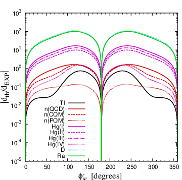
Figure 5: The observable EDMs taking |λ|=0.81|\lambda|=0.81, |κ|=0.08|\kappa|=0.08, |Aλ|=575|A_{\lambda}|=575 GeV, and |Aκ|=110|A_{\kappa}|=110 GeV. The other parameters are fixed as in Eq. (57)
Refer to caption
Refer to caption
Refer to caption
Refer to caption
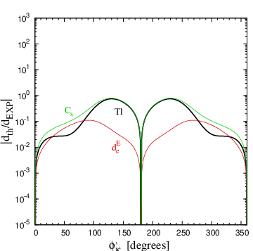
Figure 6: The observable EDMs together with the constituent contributions taking |λ|=0.81|\lambda|=0.81, |κ|=0.08|\kappa|=0.08, |Aλ|=575|A_{\lambda}|=575 GeV, and |Aκ|=110|A_{\kappa}|=110 GeV. The other parameters are fixed as in Eq. (57). Each frame shows: the Thallium EDM (upper left), the neutron EDM in the QCD sum-rule approach (upper right), the neutron EDM in the PQM (lower left), and the Mercury EDM dHgId^{\rm\,I}_{\rm Hg} (lower right).
Refer to caption
Refer to caption
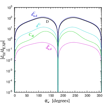
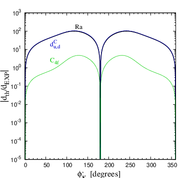
Figure 7: The observable EDMs together with the constituent contributions taking |λ|=0.81|\lambda|=0.81, |κ|=0.08|\kappa|=0.08, |Aλ|=575|A_{\lambda}|=575 GeV, and |Aκ|=110|A_{\kappa}|=110 GeV. The other parameters are fixed as in Eq. (57). The left (right) frame shows the deuteron (Radium) EDM.
Refer to caption
Refer to caption
Refer to caption
Refer to caption
Refer to caption
Refer to caption
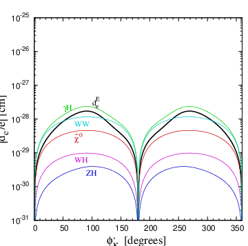
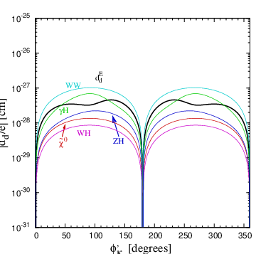
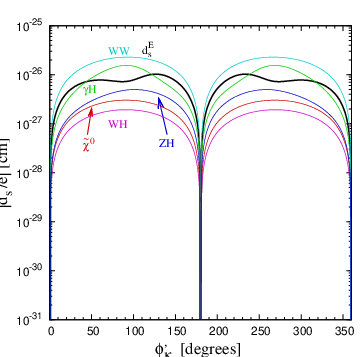
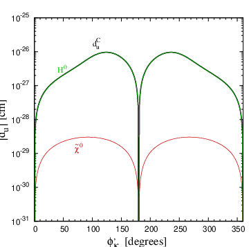
Figure 8: The EDMs and CEDMs of the electron and the light quarks together with their constituent contributions taking |λ|=0.81|\lambda|=0.81, |κ|=0.08|\kappa|=0.08, |Aλ|=575|A_{\lambda}|=575 GeV, and |Aκ|=110|A_{\kappa}|=110 GeV. The other parameters are fixed as in Eq. (57). Each frame shows |deE/e||d^{E}_{e}/e| (upper left), |duE/e||d^{E}_{u}/e| (upper right), |ddE/e||d^{E}_{d}/e| (middle left), |dsE/e||d^{E}_{s}/e| (middle right), |duC||d^{C}_{u}| (lower left), and |ddC||d^{C}_{d}| (lower right) in units of cm.

In the remaining part of this section, we wish to present the details of the observable EDMs by exemplifying a point

|λ|=0.81,|κ|=0.08,|Aλ|=575​GeV,|Aκ|=110​GeV.|\lambda|=0.81\,,\\ \ |\kappa|=0.08\,,\\ \ |A_{\lambda}|=575~~{\rm GeV}\,,\\ \ |A_{\kappa}|=110~~{\rm GeV}. (63)

The other parameters are fixed as in Eq. (57), as motivated by EWBG. In Fig. 5, we show the absolute values of the observable EDMs under consideration divided by the corresponding current experimental limits or the projected experimental sensitivities.

Fig. 6 shows the Thallium, neutron and Mercury EDMs together with the constituent contributions. We observe that both the deEd_{e}^{E} and CSC_{S} terms significantly contribute to the Thallium EDM. The dominant contributions to the neutron EDM in the QCD sum-rule approach come from the CEDM and dGd^{G} terms and we note that the neutron EDM in the CQM shows the similar behavior (not shown). The neutron EDM in the PQM is dominated by the contributions from the EDMs of the up and strange quarks. On the other hand, the Mercury EDM is dominated by the CEDMs of the light quarks. Fig. 7 shows the deuteron and Radium EDMs together with the constituent contributions. We observe both of the EDMs are dominated by the contributions from the CEDM terms.

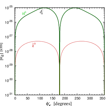
Fig. 8 shows the EDMs and CEDMS of the electron and light quarks together with the constituent contributions. We observe that the electron EDM is dominated by the two-loop Barr–Zee contributions mediated by the γ\gamma-γ\gamma-Hi0H_{i}^{0} and γ\gamma-W±W^{\pm}-W∓W^{\mp} couplings, whereas the one-loop contribution from the neutralino loops is subleading. The one-loop contribution is suppressed because the CP phase ϕκ′\phi_{\kappa}^{\prime} can contribute to EDM only through the multiple singlino-Higgsino-gaugino mixing and we are taking somewhat large values for the masses of the sfermions of the first two generations: MQ~1,2=MU~1,2=MD~1,2=ML~1,2=ME~1,2=1M_{\widetilde{Q}_{1,2}}=M_{\widetilde{U}_{1,2}}=M_{\widetilde{D}_{1,2}}=M_{\widetilde{L}_{1,2}}=M_{\widetilde{E}_{1,2}}=1 TeV. The other two-loop contributions mediated by the γ\gamma-H±H^{\pm}-W∓W^{\mp} and γ\gamma-H0H^{0}-ZZ couplings are suppressed by the large charged Higgs-boson mass ∼600\sim 600 GeV and the small vector coupling of the ZZ boson to electrons, vZ​e+​e−=−1/4+sW2v_{Ze^{+}e^{-}}=-1/4+s_{W}^{2} with sW2=0.23s_{W}^{2}=0.23, respectively.

The EDMs of the light quarks are dominated by the two-loop Barr–Zee contributions mediated by the γ\gamma-γ\gamma-Hi0H_{i}^{0} and γ\gamma-W±W^{\pm}-W∓W^{\mp} couplings. Being different from the case of deEd^{E}_{e}, the two-loop contribution mediated by the γ\gamma-H0H^{0}-ZZ couplings is larger than the one-loop contribution. We note a cancellation occurs between the two dominant two-loop Barr–Zee contributions in dd,sEd^{E}_{d,s}, resulting in |ddE|<|duE|∼|dsE||d^{E}_{d}|<|d^{E}_{u}|\sim|d^{E}_{s}|. The CEDMs of the up and down quarks are dominated by the Higgs-mediated two-loop contributions which are more than 100 times larger than the one-loop contributions and we note |ddC|/|duC|∼(md/mu)​tan⁡β∼10|d^{C}_{d}|/|d^{C}_{u}|\sim(m_{d}/m_{u})\,\tan\beta\sim 10.

Refer to caption
Figure 9: The observable EDMs taking |λ|=0.81|\lambda|=0.81, |κ|=0.08|\kappa|=0.08, |Aλ|=575|A_{\lambda}|=575 GeV, and |Aκ|=110|A_{\kappa}|=110 GeV as functions of MX~1,2≡MQ~1,2=MU~1,2=MD~1,2=ML~1,2=ME~1,2M_{\widetilde{X}_{1,2}}\equiv M_{\widetilde{Q}_{1,2}}=M_{\widetilde{U}_{1,2}}=M_{\widetilde{D}_{1,2}}=M_{\widetilde{L}_{1,2}}=M_{\widetilde{E}_{1,2}}. We have fixed ϕκ′=90∘\phi_{\kappa}^{\prime}=90^{\circ} and the other parameters are taken as in Eq. (57). The lines are the same as those in Fig. 5.

Finally, we examine the dependence of the observable EDMs on the sfermion masses of the first two generations. Fig. 9 shows the observables EDMs as functions of the common mass scale for the first two generations, MX~1,2≡MQ~1,2=MU~1,2=MD~1,2=ML~1,2=ME~1,2M_{\widetilde{X}_{1,2}}\equiv M_{\widetilde{Q}_{1,2}}=M_{\widetilde{U}_{1,2}}=M_{\widetilde{D}_{1,2}}=M_{\widetilde{L}_{1,2}}=M_{\widetilde{E}_{1,2}}. Except the neutron EDM based on the CQM which lies below the current experimental limit independently of MX~1,2M_{\widetilde{X}_{1,2}}, all the EDMs exhibit dips at certain values of MX~1,2M_{\widetilde{X}_{1,2}}. The dips occur because of the cancellation between the one- and two-loop contributions. When MX~1,2M_{\widetilde{X}_{1,2}} is small the one-loop contribution dominates. As MX~1,2M_{\widetilde{X}_{1,2}} grows, the one-loop contribution decouples and the EDMs saturate to certain values determined by the two-loop contribution. Therefore, for the neutron (QCD), Mercury, deuteron, and Radium EDMs, we observe that the one-loop contribution is comparable to or larger than the two-loop one only when MX~1,2​    <  [-0.07cm] ∼  ​300M_{\widetilde{X}_{1,2}}\raisebox{-3.69899pt}{~\shortstack{$<$ \\ [-0.07cm] $\sim$}}~300 GeV. On the other hand, for the neutron EDM based on the PQM and the Thallium EDM, the one-loop contributions are larger but the two-loop contribution starts to dominate when MX~1,2M_{\widetilde{X}_{1,2}} is larger than ∼600\sim 600 GeV. By choosing dHgIVd^{\rm\,IV}_{\rm Hg} for the Mercury EDM, we observe that all the EDM constraints could be fulfilled when MX~1,2​    >  [-0.07cm] ∼  ​300M_{\widetilde{X}_{1,2}}\raisebox{-3.69899pt}{~\shortstack{$>$ \\ [-0.07cm] $\sim$}}~300 GeV without relying on the cancellation mechanism. If we make other choices for the Mercury EDM, to suppress all the EDMs for Thallium, neutron, and Mercury below their present experimental bounds, the required degree of cancellation is about 90 % over the whole range of MX~1,2M_{\widetilde{X}_{1,2}}, with 100 % corresponding to complete cancellation.

Before we close this section, we make a comment on the tan⁡β\tan\beta dependence of the EDMs of the electron and the down and strange quarks. The one-loop neutralino contribution is proportional to tan⁡β\tan\beta. The Barr–Zee contribution mediated by the γ\gamma-W±W^{\pm}-W∓W^{\mp} couplings, one of the two two-loop leading contributions, is nearly independent of tan⁡β\tan\beta. The tan⁡β\tan\beta dependence of the other dominant Barr–Zee contribution mediated by the γ\gamma-γ\gamma-Hi0H_{i}^{0} couplings is much milder compared to the MSSM case in which the sbottom and stau contributions are proportional to tan3⁡β\tan^{3}\beta [59, 60, 49]. This is because the masses of the two heavy Higgs states, which include the CP-odd state from the Higgs doublets, increase as tan⁡β\tan\beta grows, MH4,H5≃(|λ|​vS/2)​tan⁡βM_{H_{4},H_{5}}\simeq(|\lambda|v_{S}/\sqrt{2})\,\tan\beta, to avoid tachyonic Higgs states [36].

6 Conclusions

We have performed a study on the predictions of EDMs for Thallium, neutron, Mercury, deuteron, and Radium in the framework of CP violating NMSSM. The rephasing invariant combinations of the physical CP phases contributing to the EDMs are (ϕλ′+ϕAf)(\phi_{\lambda}^{\prime}+\phi_{A_{f}}), (ϕλ′+ϕi)(\phi_{\lambda}^{\prime}+\phi_{i}), and (ϕλ′−ϕκ′)(\phi_{\lambda}^{\prime}-\phi_{\kappa}^{\prime}), with ϕAf\phi_{A_{f}} and ϕi\phi_{i} denoting the CP phases of the soft trilinear parameters AfA_{f} and the three gaugino mass parameters Mi=1,2,3M_{i=1,2,3}, respectively. Unlike the MSSM the non-vanishing CP phase (ϕλ′−ϕκ′)(\phi_{\lambda}^{\prime}-\phi_{\kappa}^{\prime}) could result in significant CP-violating mixing among the neutral Higgs bosons at tree level even when sin⁡(ϕλ′+ϕAf)=sin⁡(ϕλ′+ϕi)=0\sin(\phi_{\lambda}^{\prime}+\phi_{A_{f}})=\sin(\phi_{\lambda}^{\prime}+\phi_{i})=0. Throughout this work, we have taken a convention of ϕλ′=0\phi_{\lambda}^{\prime}=0.

The MSSM CP phases ϕAf\phi_{A_{f}} and ϕi\phi_{i} are generally known to be strongly constrained by the non-observation of the Thallium, neutron, and Mercury EDMs, without invoking cancellations among various comparable contributions, if the sfermions are within the reach of the LHC. On the other hand, the matter-dominated Universe requires sources of CP violation other than the single Kobayashi--Maskawa phase §§ § See Ref. [58] for the recently suggested bino-driven EWBG scenario exploiting the CP phase of the bino mass parameter, ϕ1\phi_{1}, to account for successful EWBG without inducing large EDMs.. In this work, we concentrate on the CP phase ϕκ′\phi_{\kappa}^{\prime}, which only exist in the NMSSM framework, by taking sin⁡(ϕAf)=sin⁡(ϕi)=0\sin(\phi_{A_{f}})=\sin(\phi_{i})=0.

One of the attractive features of the NMSSM, compared to the MSSM, might be that the mechanism of EWBG could be realized in a more natural setting. In analyzing the EDM constraint on the CP phase ϕκ′\phi_{\kappa}^{\prime}, we have taken a scenario in which a first-order phase transition is presumed to occur. The strong enough first-order phase transition is essential to the EWBG.

Previously, the constraint on ϕκ′\phi_{\kappa}^{\prime} from the neutron and electron (equivalently, Thallium) EDMs had been considered but only the one-loop neutralino contributions were taken into account. We check that our one-loop results agree well with the previous ones, showing no strong constraints on ϕκ′\phi_{\kappa}^{\prime} especially when the sfermions of the first two generations are heavier than ∼\sim 300 GeV. In this work, we have further considered the constraint from the non-observation of Mercury EDM and found the similar results.

In addition to the one-loop contributions, we have taken account of the higher-order corrections to the EDMs and CEDMs of the light quarks and electron, the dimension-six Weinberg and the Higgs-exchange four-fermion operators. We note that most of these operators are generated due to the CP-violating neutral Higgs-boson mixing induced by the CP phase ϕκ′\phi_{\kappa}^{\prime}. The two-loop contributions and, especially, the coefficient of the dimension-six Weinberg operator start to dominate when the sfermions of the first two generations are heavier than ∼\sim 300 GeV. We found that they can saturate the current bound on the neutron EDM and can go over that on the Mercury EDM. For the Mercury EDM, we have included the uncertainties in the calculation of the Schiff-moment-induced term and found that there is still a room to have the maximal CP phase ϕκ′∼90∘\phi_{\kappa}^{\prime}\sim 90^{\circ}. We have also shown that the large CP phase ϕκ′∼90∘\phi_{\kappa}^{\prime}\sim 90^{\circ} can be easily probed in the proposed future experiments searching for the EDMs of deuteron and the 225Ra atom and it might be connected to the EWBG, providing a new mechanism for it [61].

Furthermore, we offer a few more comments as follows before we close.

  1. 1.

    The new CP phase that we considered here can be applied to a number of low-energy phenomenologies, such as CP asymmetries in BB mesons and KK mesons.

  2. 2.

    In our previous work [36], we have imposed the following constraints to the parameter space: the LEP limits, the global minimum condition, and the positivity of the square of the Higgs-boson masses. In the present work, we have further constrained the parameter space required by the EDM constraints. Therefore, by combining all these constraints we can explore further phenomenologies, including the Higgs physics at the LHC, the muon anomalous magnetic moment, and electroweak baryogenesis.

  3. 3.

    One of the reasons why the 2-loop BZ diagrams can dominate is that one or more of the neutral Higgs bosons become very light. One can imagine that contributions to the muon anomalous magnetic moments can also become important in comparison to the one-loop result. In fact, one can show that the muon anomalous magnetic moment and EDM are related to the real and imaginary parts of the combination of couplings. We will come back to this issue in a future work.

  4. 4.

    We will soon make available a computer code for calculating all the couplings and masses of the Higgs bosons, with the parameter space restricted by all the experimental constraints (all the above mentioned ones as well as direct search limits, muon g−2g-2, etc) as we proceed further in this framework.

Acknowledgements

The work was supported in parts by the NSC of Taiwan (grant No. 99-2112-M-007-005-MY3), the NCTS, and by the WCU program through the KOSEF funded by the MEST (R31-2008-000-10057-0).

Appendices

Throughout Appendices, we are following the conventions and notations of CPsuperH [27].

Appendix A Masses and mixing matrices

Here we set up our conventions and notations of the masses and mixing matrices of neutral Higgs bosons, charginos, neutralinos, third-generations sfermions.

  • •

    Neutral Higgs bosons:

    (ϕd0,ϕu0,ϕS0,a,aS)αT=Oα​i​(H1,H2,H3,H4,H5)iT,(\phi_{d}^{0},\phi_{u}^{0},\phi_{S}^{0},a,a_{S})^{T}_{\alpha}=O_{\alpha i}(H_{1},H_{2},H_{3},H_{4},H_{5})^{T}_{i}\,, (A.1)

    where OT​ℳH2​O=𝖽𝗂𝖺𝗀⁡(MH12,MH22,MH32,MH42,MH52)O^{T}{\cal M}^{2}_{H}\,O={\sf diag}\,(M^{2}_{H_{1}},M^{2}_{H_{2}},M^{2}_{H_{3}},M^{2}_{H_{4}},M^{2}_{H_{5}}) with MH1≤MH2≤MH3≤MH4≤MH5M_{H_{1}}\leq M_{H_{2}}\leq M_{H_{3}}\leq M_{H_{4}}\leq M_{H_{5}}.

  • •

    Charginos: We adopt the convention H~L⁡(R)−=H~d⁡(u)−\widetilde{H}^{-}_{L(R)}=\widetilde{H}^{-}_{d(u)}. The chargino mass matrix in the (W~−,H~−)(\widetilde{W}^{-},\widetilde{H}^{-}) basis

    ℳC=(M22​MW​cβ2​MW​sβ|λ|​vS2​ei⁡(ϕλ+θ+φ)),\displaystyle{\cal M}_{C}=\left(\begin{array}[]{cc}M_{2}&\sqrt{2}M_{W}\,c_{\beta}\\[5.69054pt] \sqrt{2}M_{W}\,s_{\beta}&\frac{|\lambda|v_{S}}{\sqrt{2}}\,e^{i(\phi_{\lambda}+\theta+\varphi)}\end{array}\right)\,,

    is diagonalized by two different unitary matrices CR​ℳC​CL†=𝖽𝗂𝖺𝗀⁡{mχ~1±,mχ~2±}C_{R}{\cal M}_{C}C_{L}^{\dagger}={\sf diag}\{m_{\widetilde{\chi}^{\pm}_{1}},\,m_{\widetilde{\chi}^{\pm}_{2}}\}, where mχ~1±≤mχ~2±m_{\widetilde{\chi}^{\pm}_{1}}\leq m_{\widetilde{\chi}^{\pm}_{2}}. The chargino mixing matrices (CL)i​α(C_{L})_{i\alpha} and (CR)i​α(C_{R})_{i\alpha} relate the electroweak eigenstates to the mass eigenstates, via

    χ~α​L−\displaystyle\widetilde{\chi}^{-}_{\alpha L} =\displaystyle= (CL)i​α∗​χ~i​L−,χ~α​L−=(W~−,H~−)LT,\displaystyle(C_{L})^{*}_{i\alpha}\widetilde{\chi}_{iL}^{-}\,,\qquad\widetilde{\chi}^{-}_{\alpha L}\ =\ (\widetilde{W}^{-},\widetilde{H}^{-})_{L}^{T}\,,
    χ~α​R−\displaystyle\widetilde{\chi}^{-}_{\alpha R} =\displaystyle= (CR)i​α∗​χ~i​R−,χ~α​R−=(W~−,H~−)RT.\displaystyle(C_{R})^{*}_{i\alpha}\widetilde{\chi}_{iR}^{-}\,,\qquad\widetilde{\chi}^{-}_{\alpha R}\ =\ (\widetilde{W}^{-},\widetilde{H}^{-})_{R}^{T}\,. (A.5)

    We use the following abbreviations throughout this paper: sβ≡sin⁡βs_{\beta}\equiv\sin\beta, cβ≡cos⁡βc_{\beta}\equiv\cos\beta, tβ=tan⁡βt_{\beta}=\tan\beta, s2​β≡sin⁡ 2​βs_{2\beta}\equiv\sin\,2\beta, c2​β≡cos⁡ 2​βc_{2\beta}\equiv\cos\,2\beta, sW≡sin⁡θWs_{W}\equiv\sin\theta_{W}, cW≡cos⁡θWc_{W}\equiv\cos\theta_{W}, etc.

  • •

    Neutralinos: The symmetric neutralino mass matrix in the (B~,W~0,H~d0,H~u0,S~)(\widetilde{B},\widetilde{W}^{0},\widetilde{H}^{0}_{d},\widetilde{H}^{0}_{u},\widetilde{S}) basis is given by

    ℳN=(M10−MZ​cβ​sWMZ​sβ​sW0M2MZ​cβ​cW−MZ​sβ​cW00−|λ|​vS2​ei⁡(ϕλ+θ+φ)−|λ|​v​sβ2​ei⁡(ϕλ+θ+φ)0−|λ|​v​cβ2​ei⁡(ϕλ+θ+φ)2​|κ|​vS​ei⁡(ϕκ+3​φ))\displaystyle{\cal M}_{N}=\left(\begin{array}[]{ccccc}M_{1}&0&-M_{Z}c_{\beta}s_{W}&M_{Z}s_{\beta}s_{W}&0\\[5.69054pt] &M_{2}&M_{Z}c_{\beta}c_{W}&-M_{Z}s_{\beta}c_{W}&0\\[5.69054pt] &&0&-\frac{|\lambda|v_{S}}{\sqrt{2}}\,e^{i(\phi_{\lambda}+\theta+\varphi)}&-\frac{|\lambda|vs_{\beta}}{\sqrt{2}}\,e^{i(\phi_{\lambda}+\theta+\varphi)}\\[5.69054pt] &&&0&-\frac{|\lambda|vc_{\beta}}{\sqrt{2}}\,e^{i(\phi_{\lambda}+\theta+\varphi)}\\[5.69054pt] &&&&\sqrt{2}|\kappa|v_{S}\,e^{i(\phi_{\kappa}+3\varphi)}\end{array}\right)\,

    This neutralino mass matrix is diagonalized by a unitary matrix NN: N∗​ℳN​N†=𝖽𝗂𝖺𝗀⁡(mχ~10,mχ~20,mχ~30,mχ~40,mχ~50)N^{*}{\cal M}_{N}N^{\dagger}={\sf diag}\,(m_{\widetilde{\chi}_{1}^{0}},m_{\widetilde{\chi}_{2}^{0}},m_{\widetilde{\chi}_{3}^{0}},m_{\widetilde{\chi}_{4}^{0}},m_{\widetilde{\chi}_{5}^{0}}) with mχ~10≤mχ~20≤mχ~30≤mχ~40≤mχ~50m_{\widetilde{\chi}_{1}^{0}}\leq m_{\widetilde{\chi}_{2}^{0}}\leq m_{\widetilde{\chi}_{3}^{0}}\leq m_{\widetilde{\chi}_{4}^{0}}\leq m_{\widetilde{\chi}_{5}^{0}}. The neutralino mixing matrix Ni​αN_{i\alpha} relates the electroweak eigenstates to the mass eigenstates via

    (B~,W~0,H~d0,H~u0,S~)αT=Ni​α∗​(χ~10,χ~20,χ~30,χ~40,χ~50)iT.\displaystyle(\widetilde{B},\widetilde{W}^{0},\widetilde{H}^{0}_{d},\widetilde{H}^{0}_{u},\widetilde{S})^{T}_{\alpha}=N_{i\alpha}^{*}({\widetilde{\chi}_{1}^{0}},{\widetilde{\chi}_{2}^{0}},{\widetilde{\chi}_{3}^{0}},{\widetilde{\chi}_{4}^{0}},{\widetilde{\chi}_{5}^{0}})^{T}_{i}\,. (A.12)
  • •

    Stops, sbottoms, staus and tau sneutrino: At the tree level, the Yukawa couplings are given by

    hl=2​mlv​cβ;hd=2​mdv​cβ;hu=e−i​θ​2​muv​sβ.h_{l}=\frac{\sqrt{2}\,m_{l}}{vc_{\beta}}\,;\ \ \ h_{d}=\frac{\sqrt{2}\,m_{d}}{vc_{\beta}}\,;\ \ \ h_{u}=e^{-i\theta}\,\frac{\sqrt{2}\,m_{u}}{vs_{\beta}}\,. (A.13)

    The stop and sbottom mass matrices may conveniently be written in the (q~L,q~R)\left(\widetilde{q}_{L},\widetilde{q}_{R}\right) basis as

    ℳ~t2\displaystyle\hskip-14.22636pt\widetilde{\cal M}^{2}_{t} =\displaystyle= (MQ~32+mt2+c2​β​MZ2​(T3​Lt−Qt​sW2)ht∗​vu​(Au∗​e−i​θ−|λ|​vS2​ei⁡(ϕλ+φ)​cot⁡β)/2ht​vu​(Au​ei​θ−|λ|​vS2​e−i⁡(ϕλ+φ)​cot⁡β)/2MU~32+mt2+c2​β​MZ2​Qt​sW2),\displaystyle\left(\begin{array}[]{cc}M^{2}_{\widetilde{Q}_{3}}\,+\,m^{2}_{t}\,+\,c_{2\beta}M^{2}_{Z}\,(T^{t}_{3L}\,-\,Q_{t}s_{W}^{2})&h_{t}^{*}v_{u}(A^{*}_{u}e^{-i\theta}-\frac{|\lambda|v_{S}}{\sqrt{2}}e^{i(\phi_{\lambda}+\varphi)}\cot\beta)/\sqrt{2}\\ h_{t}v_{u}(A_{u}e^{i\theta}-\frac{|\lambda|v_{S}}{\sqrt{2}}e^{-i(\phi_{\lambda}+\varphi)}\cot\beta)/\sqrt{2}&\hskip-5.69046ptM^{2}_{\widetilde{U}_{3}}\,+\,m^{2}_{t}\,+\,c_{2\beta}M^{2}_{Z}\,Q_{t}s^{2}_{W}\end{array}\right)\,,
    ℳ~b2\displaystyle\hskip-14.22636pt\widetilde{\cal M}^{2}_{b} =\displaystyle= (MQ~32+mb2+c2​β​MZ2​(T3​Lb−Qb​sW2)hb∗​vd​(Ab∗−|λ|​vS2​ei⁡(ϕλ+θ+φ)​tan⁡β)/2hb​vd​(Ab−|λ|​vS2​e−i⁡(ϕλ+θ+φ)​tan⁡β)/2MD~32+mb2+c2​β​MZ2​Qb​sW2),\displaystyle\left(\begin{array}[]{cc}M^{2}_{\widetilde{Q}_{3}}\,+\,m^{2}_{b}\,+\,c_{2\beta}M^{2}_{Z}\,(T^{b}_{3L}\,-\,Q_{b}s_{W}^{2})&h_{b}^{*}v_{d}(A^{*}_{b}-\frac{|\lambda|v_{S}}{\sqrt{2}}e^{i(\phi_{\lambda}+\theta+\varphi)}\tan\beta)/\sqrt{2}\\ h_{b}v_{d}(A_{b}-\frac{|\lambda|v_{S}}{\sqrt{2}}e^{-i(\phi_{\lambda}+\theta+\varphi)}\tan\beta)/\sqrt{2}&\hskip-5.69046ptM^{2}_{\widetilde{D}_{3}}\,+\,m^{2}_{b}\,+\,c_{2\beta}M^{2}_{Z}\,Q_{b}s^{2}_{W}\end{array}\right)\,,

    with T3​Lt=−T3​Lb=1/2T^{t}_{3L}=-T^{b}_{3L}=1/2, Qt=2/3Q_{t}=2/3, Qb=−1/3Q_{b}=-1/3, and hqh_{q} is the Yukawa coupling of the quark qq. On the other hand, the stau mass matrix is written in the (τ~L,τ~R)\left(\widetilde{\tau}_{L},\widetilde{\tau}_{R}\right) basis as

    ℳ~τ2=(ML~32+mτ2+c2​β​MZ2​(sW2−1/2)hτ∗​vd​(Aτ∗−|λ|​vS2​ei⁡(ϕλ+θ+φ)​tan⁡β)/2hτ​vd​(Aτ−|λ|​vS2​e−i⁡(ϕλ+θ+φ)​tan⁡β)/2ME~32+mτ2−c2​β​MZ2​sW2),\hskip-14.22636pt\widetilde{\cal M}^{2}_{\tau}=\left(\begin{array}[]{cc}M^{2}_{\widetilde{L}_{3}}\,+\,m^{2}_{\tau}\,+\,c_{2\beta}M^{2}_{Z}\,(s_{W}^{2}-1/2)&h_{\tau}^{*}v_{d}(A^{*}_{\tau}-\frac{|\lambda|v_{S}}{\sqrt{2}}e^{i(\phi_{\lambda}+\theta+\varphi)}\tan\beta)/\sqrt{2}\\ h_{\tau}v_{d}(A_{\tau}-\frac{|\lambda|v_{S}}{\sqrt{2}}e^{-i(\phi_{\lambda}+\theta+\varphi)}\tan\beta)/\sqrt{2}&\hskip-5.69046ptM^{2}_{\widetilde{E}_{3}}\,+\,m^{2}_{\tau}\,-\,c_{2\beta}M^{2}_{Z}\,s^{2}_{W}\end{array}\right)\,, (A.21)

    and the mass of the tau sneutrino ντ~\widetilde{\nu_{\tau}} is simply mν~τ=ML~32+12​c2​β​MZ2m_{\widetilde{\nu}_{\tau}}=\sqrt{M^{2}_{\widetilde{L}_{3}}+\frac{1}{2}c_{2\beta}M_{Z}^{2}}, as it has no right–handed counterpart in the NMSSM as in the MSSM.

    The 2×22\times 2 sfermion mass matrix ℳ~f2\widetilde{\cal M}^{2}_{f} for f=t,bf=t,b and τ\tau is diagonalized by a unitary matrix Uf~U^{\widetilde{f}}: Uf~†ℳ~f2Uf~=𝖽𝗂𝖺𝗀(mf~12,mf~22)U^{\widetilde{f}\dagger}\,\widetilde{\cal M}^{2}_{f}\,U^{\widetilde{f}}={\sf diag}(m_{\widetilde{f}_{1}}^{2},m_{\widetilde{f}_{2}}^{2})\, with mf~12≤mf~22m_{\widetilde{f}_{1}}^{2}\leq m_{\widetilde{f}_{2}}^{2}. The mixing matrix Uf~U^{\widetilde{f}} relates the electroweak eigenstates f~L,R\widetilde{f}_{L,R} to the mass eigenstates f~1,2\widetilde{f}_{1,2}, via

    (f~L,f~R)αT=Uα​if~​(f~1,f~2)iT.(\widetilde{f}_{L},\widetilde{f}_{R})^{T}_{\alpha}\,=\,U^{\widetilde{f}}_{\alpha i}\,(\widetilde{f}_{1},\widetilde{f}_{2})^{T}_{i}\,. (A.22)

Appendix B Higgs-boson couplings to sfermions

Here we present the couplings of the neutral and charged Higgs bosons to squarks and sleptons in the weak basis.

  • •

    The neutral Higgs couplings to sfermions:

    • –

      In the (b~L,b~R)(\widetilde{b}_{L},\widetilde{b}_{R}) basis, the neutral Higgs couplings to the sbottoms:

      Γϕd0​b~∗​b~\displaystyle\Gamma^{\phi_{d}^{0}\,\widetilde{b}^{*}\widetilde{b}} =\displaystyle= (−|hb|2​v​cβ+14​(g2+13​g′2)​v​cβ−12​hb∗​Ab∗−12​hb​Ab−|hb|2​v​cβ+16​g′2​v​cβ),\displaystyle\left(\begin{array}[]{cc}-|h_{b}|^{2}vc_{\beta}+\frac{1}{4}\left(g^{2}+\frac{1}{3}g^{\prime 2}\right)vc_{\beta}&-\frac{1}{\sqrt{2}}h_{b}^{*}A_{b}^{*}\\[5.69054pt] -\frac{1}{\sqrt{2}}h_{b}A_{b}&-|h_{b}|^{2}vc_{\beta}+\frac{1}{6}g^{\prime 2}vc_{\beta}\end{array}\right)\,,
      Γϕu0​b~∗​b~\displaystyle\Gamma^{\phi_{u}^{0}\widetilde{b}^{*}\widetilde{b}} =\displaystyle= (−14​(g2+13​g′2)​v​sβ12​hb∗​|λ|​vS​ei⁡(ϕλ+θ+φ)12​hb​|λ|​vS​e−i⁡(ϕλ+θ+φ)−16​g′2​v​sβ),\displaystyle\left(\begin{array}[]{cc}-\frac{1}{4}\left(g^{2}+\frac{1}{3}g^{\prime 2}\right)vs_{\beta}&\frac{1}{2}h_{b}^{*}|\lambda|v_{S}\,e^{i(\phi_{\lambda}+\theta+\varphi)}\\[5.69054pt] \frac{1}{2}h_{b}|\lambda|v_{S}\,e^{-i(\phi_{\lambda}+\theta+\varphi)}&-\frac{1}{6}g^{\prime 2}vs_{\beta}\end{array}\right)\,,
      ΓϕS0​b~∗​b~\displaystyle\Gamma^{\phi_{S}^{0}\,\widetilde{b}^{*}\widetilde{b}} =\displaystyle= (012​hb∗​|λ|​v​sβ​ei⁡(ϕλ+θ+φ)12​hb​|λ|​v​sβ​e−i⁡(ϕλ+θ+φ)0),\displaystyle\left(\begin{array}[]{cc}0&\frac{1}{2}\,h_{b}^{*}|\lambda|\,v\,s_{\beta}\,e^{i(\phi_{\lambda}+\theta+\varphi)}\\[5.69054pt] \frac{1}{2}\,h_{b}|\lambda|\,v\,s_{\beta}\,e^{-i(\phi_{\lambda}+\theta+\varphi)}&0\end{array}\right)\,,
      Γa​b~∗​b~\displaystyle\Gamma^{a\,\widetilde{b}^{*}\widetilde{b}} =\displaystyle= 12​(0i​hb∗​(sβ​Ab∗+cβ​|λ|​vS2​ei⁡(ϕλ+θ+φ))−i​hb​(sβ​Ab+cβ​|λ|​vS2​e−i⁡(ϕλ+θ+φ))0),\displaystyle\frac{1}{\sqrt{2}}\left(\begin{array}[]{cc}0&i\,h_{b}^{*}\left(s_{\beta}A_{b}^{*}+c_{\beta}\frac{|\lambda|\,v_{S}}{\sqrt{2}}\,e^{i(\phi_{\lambda}+\theta+\varphi)}\right)\\[5.69054pt] -i\,h_{b}\left(s_{\beta}A_{b}+c_{\beta}\frac{|\lambda|\,v_{S}}{\sqrt{2}}\,e^{-i(\phi_{\lambda}+\theta+\varphi)}\right)&0\end{array}\right)\,,
      ΓaS​b~∗​b~\displaystyle\Gamma^{a_{S}\,\widetilde{b}^{*}\widetilde{b}} =\displaystyle= (0i​12​hb∗​|λ|​v​sβ​ei⁡(ϕλ+θ+φ)−i​12​hb​|λ|​v​sβ​e−i⁡(ϕλ+θ+φ)0),\displaystyle\left(\begin{array}[]{cc}0&i\,\frac{1}{2}\,h_{b}^{*}|\lambda|\,v\,s_{\beta}\,e^{i(\phi_{\lambda}+\theta+\varphi)}\\[5.69054pt] -i\,\frac{1}{2}\,h_{b}|\lambda|\,v\,s_{\beta}\,e^{-i(\phi_{\lambda}+\theta+\varphi)}&0\end{array}\right)\,,
    • –

      In the (t~L,t~R)(\widetilde{t}_{L},\widetilde{t}_{R}) basis, the neutral Higgs couplings to the stops:

      Γϕd0​t~∗​t~\displaystyle\Gamma^{\phi_{d}^{0}\,\widetilde{t}^{*}\widetilde{t}} =\displaystyle= (−14​(g2−13​g′2)​v​cβ12​ht∗​|λ|​vS​ei⁡(ϕλ+φ)12​ht​|λ|​vS​e−i⁡(ϕλ+φ)−13​g′2​v​cβ),\displaystyle\left(\begin{array}[]{cc}-\frac{1}{4}\left(g^{2}-\frac{1}{3}g^{\prime 2}\right)vc_{\beta}&\frac{1}{2}h_{t}^{*}|\lambda|v_{S}\,e^{i(\phi_{\lambda}+\varphi)}\\[5.69054pt] \frac{1}{2}h_{t}|\lambda|v_{S}\,e^{-i(\phi_{\lambda}+\varphi)}&-\frac{1}{3}g^{\prime 2}vc_{\beta}\end{array}\right)\,,
      Γϕu0​t~∗​t~\displaystyle\Gamma^{\phi_{u}^{0}\,\widetilde{t}^{*}\widetilde{t}} =\displaystyle= (−|ht|2​v​sβ+14​(g2−13​g′2)​v​sβ−12​ht∗​At∗​e−i​θ−12​ht​At​ei​θ−|ht|2​v​sβ+13​g′2​v​sβ),\displaystyle\left(\begin{array}[]{cc}-|h_{t}|^{2}vs_{\beta}+\frac{1}{4}\left(g^{2}-\frac{1}{3}g^{\prime 2}\right)vs_{\beta}&-\frac{1}{\sqrt{2}}h_{t}^{*}A_{t}^{*}\,e^{-i\theta}\\[5.69054pt] -\frac{1}{\sqrt{2}}h_{t}A_{t}\,e^{i\theta}&-|h_{t}|^{2}vs_{\beta}+\frac{1}{3}g^{\prime 2}vs_{\beta}\end{array}\right)\,,
      ΓϕS0​t~∗​t~\displaystyle\Gamma^{\phi_{S}^{0}\,\widetilde{t}^{*}\widetilde{t}} =\displaystyle= (012​ht∗​|λ|​v​cβ​ei⁡(ϕλ+φ)12​ht​|λ|​v​cβ​e−i⁡(ϕλ+φ)0),\displaystyle\left(\begin{array}[]{cc}0&\frac{1}{2}\,h_{t}^{*}|\lambda|\,v\,c_{\beta}\,e^{i(\phi_{\lambda}+\varphi)}\\[5.69054pt] \frac{1}{2}\,h_{t}|\lambda|\,v\,c_{\beta}\,e^{-i(\phi_{\lambda}+\varphi)}&0\end{array}\right)\,,
      Γa​t~∗​t~\displaystyle\Gamma^{a\,\widetilde{t}^{*}\widetilde{t}} =\displaystyle= 12​(0i​ht∗​(cβ​At∗​e−i​θ+sβ​|λ|​vS2​ei⁡(ϕλ+φ))−i​ht​(cβ​At​ei​θ+sβ​|λ|​vS2​e−i⁡(ϕλ+φ))0),\displaystyle\frac{1}{\sqrt{2}}\left(\begin{array}[]{cc}0&i\,h_{t}^{*}\left(c_{\beta}A_{t}^{*}\,e^{-i\theta}+s_{\beta}\frac{|\lambda|\,v_{S}}{\sqrt{2}}\,e^{i(\phi_{\lambda}+\varphi)}\right)\\[5.69054pt] -i\,h_{t}\left(c_{\beta}A_{t}\,e^{i\theta}+s_{\beta}\frac{|\lambda|\,v_{S}}{\sqrt{2}}\,e^{-i(\phi_{\lambda}+\varphi)}\right)&0\end{array}\right)\,,
      ΓaS​t~∗​t~\displaystyle\Gamma^{a_{S}\,\widetilde{t}^{*}\widetilde{t}} =\displaystyle= (0i​12​ht∗​|λ|​v​cβ​ei⁡(ϕλ+φ)−i​12​ht​|λ|​v​cβ​e−i⁡(ϕλ+φ)0),\displaystyle\left(\begin{array}[]{cc}0&i\,\frac{1}{2}\,h_{t}^{*}|\lambda|\,v\,c_{\beta}\,e^{i(\phi_{\lambda}+\varphi)}\\[5.69054pt] -i\,\frac{1}{2}\,h_{t}|\lambda|\,v\,c_{\beta}\,e^{-i(\phi_{\lambda}+\varphi)}&0\end{array}\right)\,,
    • –

      In the (τ~L,τ~R)(\widetilde{\tau}_{L},\widetilde{\tau}_{R}) basis, the neutral Higgs couplings to the staus:

      Γϕd0​τ~∗​τ~\displaystyle\Gamma^{\phi_{d}^{0}\,\widetilde{\tau}^{*}\widetilde{\tau}} =\displaystyle= (−|hτ|2​v​cβ+14​(g2−g′2)​v​cβ−12​hτ∗​Aτ∗−12​hτ​Aτ−|hτ|2​v​cβ+12​g′2​v​cβ),\displaystyle\left(\begin{array}[]{cc}-|h_{\tau}|^{2}vc_{\beta}+\frac{1}{4}\left(g^{2}-g^{\prime 2}\right)vc_{\beta}&-\frac{1}{\sqrt{2}}h_{\tau}^{*}A_{\tau}^{*}\\[5.69054pt] -\frac{1}{\sqrt{2}}h_{\tau}A_{\tau}&-|h_{\tau}|^{2}vc_{\beta}+\frac{1}{2}g^{\prime 2}vc_{\beta}\end{array}\right)\,,
      Γϕu0​τ~∗​τ~\displaystyle\Gamma^{\phi_{u}^{0}\widetilde{\tau}^{*}\widetilde{\tau}} =\displaystyle= (−14​(g2−g′2)​v​sβ12​hτ∗​|λ|​vS​ei⁡(ϕλ+θ+φ)12​hτ​|λ|​vS​e−i⁡(ϕλ+θ+φ)−12​g′2​v​sβ),\displaystyle\left(\begin{array}[]{cc}-\frac{1}{4}\left(g^{2}-g^{\prime 2}\right)vs_{\beta}&\frac{1}{2}h_{\tau}^{*}|\lambda|v_{S}\,e^{i(\phi_{\lambda}+\theta+\varphi)}\\[5.69054pt] \frac{1}{2}h_{\tau}|\lambda|v_{S}\,e^{-i(\phi_{\lambda}+\theta+\varphi)}&-\frac{1}{2}g^{\prime 2}vs_{\beta}\end{array}\right)\,,
      ΓϕS0​τ~∗​τ~\displaystyle\Gamma^{\phi_{S}^{0}\,\widetilde{\tau}^{*}\widetilde{\tau}} =\displaystyle= (012​hτ∗​|λ|​v​sβ​ei⁡(ϕλ+θ+φ)12​hτ​|λ|​v​sβ​e−i⁡(ϕλ+θ+φ)0),\displaystyle\left(\begin{array}[]{cc}0&\frac{1}{2}\,h_{\tau}^{*}|\lambda|\,v\,s_{\beta}\,e^{i(\phi_{\lambda}+\theta+\varphi)}\\[5.69054pt] \frac{1}{2}\,h_{\tau}|\lambda|\,v\,s_{\beta}\,e^{-i(\phi_{\lambda}+\theta+\varphi)}&0\end{array}\right)\,,
      Γa​τ~∗​τ~\displaystyle\Gamma^{a\,\widetilde{\tau}^{*}\widetilde{\tau}} =\displaystyle= 12​(0i​hτ∗​(sβ​Aτ∗+cβ​|λ|​vS2​ei⁡(ϕλ+θ+φ))−i​hτ​(sβ​Aτ+cβ​|λ|​vS2​e−i⁡(ϕλ+θ+φ))0),\displaystyle\frac{1}{\sqrt{2}}\left(\begin{array}[]{cc}0&i\,h_{\tau}^{*}\left(s_{\beta}A_{\tau}^{*}+c_{\beta}\frac{|\lambda|\,v_{S}}{\sqrt{2}}\,e^{i(\phi_{\lambda}+\theta+\varphi)}\right)\\[5.69054pt] -i\,h_{\tau}\left(s_{\beta}A_{\tau}+c_{\beta}\frac{|\lambda|\,v_{S}}{\sqrt{2}}\,e^{-i(\phi_{\lambda}+\theta+\varphi)}\right)&0\end{array}\right)\,,
      ΓaS​τ~∗​τ~\displaystyle\Gamma^{a_{S}\,\widetilde{\tau}^{*}\widetilde{\tau}} =\displaystyle= (0i​12​hτ∗​|λ|​v​sβ​ei⁡(ϕλ+θ+φ)−i​12​hτ​|λ|​v​sβ​e−i⁡(ϕλ+θ+φ)0),\displaystyle\left(\begin{array}[]{cc}0&i\,\frac{1}{2}\,h_{\tau}^{*}|\lambda|\,v\,s_{\beta}\,e^{i(\phi_{\lambda}+\theta+\varphi)}\\[5.69054pt] -i\,\frac{1}{2}\,h_{\tau}|\lambda|\,v\,s_{\beta}\,e^{-i(\phi_{\lambda}+\theta+\varphi)}&0\end{array}\right)\,,
    • –

      The neutral Higgs couplings to the sneutrinos

      Γϕ1​ν~τ∗​ν~τ=−14​(g2+g′2)​v​cβ,Γϕ2​ν~τ∗​ν~τ=14​(g2+g′2)​v​sβ,\displaystyle\Gamma^{\phi_{1}\widetilde{\nu}^{*}_{\tau}\widetilde{\nu}_{\tau}}=-\frac{1}{4}\left(g^{2}+g^{\prime 2}\right)vc_{\beta},\qquad\Gamma^{\phi_{2}\widetilde{\nu}^{*}_{\tau}\widetilde{\nu}_{\tau}}=\frac{1}{4}\left(g^{2}+g^{\prime 2}\right)vs_{\beta}\,,

      and the other couplings are vanishing.

  • •

    The charged Higgs couplings to sfermions:

    ΓH+​u~∗​d~\displaystyle\Gamma^{H^{+}\widetilde{u}^{*}\widetilde{d}}\ =\displaystyle= (12​(|hu|2+|hd|2−g2)​v​sβ​cβhd∗​(sβ​Ad∗+cβ​|λ|​vS2​ei⁡(ϕλ+θ+φ))hu​(cβ​Au​ei​θ+sβ​|λ|​vS2​e−i⁡(ϕλ+φ))12​hu​hd∗​v)\displaystyle\ \left(\begin{array}[]{cc}\frac{1}{\sqrt{2}}\,(|h_{u}|^{2}+|h_{d}|^{2}-g^{2})\,vs_{\beta}c_{\beta}&h_{d}^{*}\,\left(s_{\beta}A^{*}_{d}+c_{\beta}\frac{|\lambda|\,v_{S}}{\sqrt{2}}\,e^{i(\phi_{\lambda}+\theta+\varphi)}\right)\\[5.69054pt] h_{u}\,\left(c_{\beta}A_{u}\,e^{i\theta}+s_{\beta}\frac{|\lambda|\,v_{S}}{\sqrt{2}}\,e^{-i(\phi_{\lambda}+\varphi)}\right)&\frac{1}{\sqrt{2}}\,h_{u}h^{*}_{d}\,v\end{array}\right)\,
    ΓH+​ν~τ∗​τ~L\displaystyle\Gamma^{H^{+}\widetilde{\nu}_{\tau}^{*}\widetilde{\tau}_{L}}\ =\displaystyle= 12​(|hτ|2−g2)​v​sβ​cβ,ΓH+​ν~τ∗​τ~R=hτ∗​(sβ​Aτ∗+cβ​|λ|​vS2​ei⁡(ϕλ+θ+φ)).\displaystyle\ \frac{1}{\sqrt{2}}\,(|h_{\tau}|^{2}-g^{2})\,vs_{\beta}\,c_{\beta}\,,\qquad\Gamma^{H^{+}\widetilde{\nu}_{\tau}^{*}\widetilde{\tau}_{R}}\ =\ h^{*}_{\tau}\left(s_{\beta}A^{*}_{\tau}+c_{\beta}\frac{|\lambda|\,v_{S}}{\sqrt{2}}\,e^{i(\phi_{\lambda}+\theta+\varphi)}\right)\,.

References

  • [1] M. Dine, W. Fischler and M. Srednicki, Phys. Lett. B 104 (1981) 199; H. P. Nilles, M. Srednicki and D. Wyler, Phys. Lett. B 120 (1983) 346; J. M. Frere, D. R. T. Jones and S. Raby, Nucl. Phys. B 222 (1983) 11; A. I. Veselov, M. I. Vysotsky and K. A. Ter-Martirosian, Sov. Phys. JETP 63 (1986) 489 [Zh. Eksp. Teor. Fiz. 90 (1986) 838]; J. P. Derendinger and C. A. Savoy, Nucl. Phys. B 237 (1984) 307.
  • [2] J. R. Ellis, J. F. Gunion, H. E. Haber, L. Roszkowski and F. Zwirner, Phys. Rev. D 39 (1989) 844; U. Ellwanger, Phys. Lett. B 303 (1993) 271 [arXiv:hep-ph/9302224]; U. Ellwanger, M. Rausch de Traubenberg and C. A. Savoy, Phys. Lett. B 315 (1993) 331 [arXiv:hep-ph/9307322]; P. N. Pandita, Phys. Lett. B 318 (1993) 338; P. N. Pandita, Z. Phys. C 59 (1993) 575; T. Elliott, S. F. King and P. L. White, Phys. Rev. D 49 (1994) 2435 [arXiv:hep-ph/9308309]; G. K. Yeghian, arXiv:hep-ph/9904488; S. F. King and P. L. White, Phys. Rev. D 52 (1995) 4183 [arXiv:hep-ph/9505326]; U. Ellwanger, M. Rausch de Traubenberg and C. A. Savoy, Nucl. Phys. B 492 (1997) 21 [arXiv:hep-ph/9611251]; F. Franke and H. Fraas, Int. J. Mod. Phys. A 12 (1997) 479 [arXiv:hep-ph/9512366]; B. Ananthanarayan and P. N. Pandita, Int. J. Mod. Phys. A 12 (1997) 2321 [arXiv:hep-ph/9601372]; U. Ellwanger and C. Hugonie, Eur. Phys. J. C 25 (2002) 297 [arXiv:hep-ph/9909260]; U. Ellwanger, J. F. Gunion, C. Hugonie and S. Moretti, arXiv:hep-ph/0305109; U. Ellwanger and C. Hugonie, Phys. Lett. B 623 (2005) 93 [arXiv:hep-ph/0504269].
  • [3] M. Matsuda and M. Tanimoto, Phys. Rev. D 52 (1995) 3100 [arXiv:hep-ph/9504260]; N. Haba, Prog. Theor. Phys. 97 (1997) 301 [arXiv:hep-ph/9608357]; S. W. Ham, J. Kim, S. K. Oh and D. Son, Phys. Rev. D 64 (2001) 035007 [arXiv:hep-ph/0104144]; S. W. Ham, S. K. Oh and D. Son, Phys. Rev. D 65 (2002) 075004 [arXiv:hep-ph/0110052]; S. W. Ham, S. H. Kim, S. K. OH and D. Son, Phys. Rev. D 76 (2007) 115013 [arXiv:0708.2755 [hep-ph]].
  • [4] M. Boz, Mod. Phys. Lett. A 21 (2006) 243 [arXiv:hep-ph/0511072].
  • [5] G. Degrassi and P. Slavich, Nucl. Phys. B 825, 119 (2010) [arXiv:0907.4682 [hep-ph]].
  • [6] For recent reviews on the NMSSM, see, U. Ellwanger, C. Hugonie and A. M. Teixeira, arXiv:0910.1785 [hep-ph]; S. Chang, R. Dermisek, J. F. Gunion and N. Weiner, Ann. Rev. Nucl. Part. Sci. 58, 75 (2008) [arXiv:0801.4554 [hep-ph]].
  • [7] J. E. Kim and H. P. Nilles, Phys. Lett. B 138, 150 (1984); Y. Nir, Phys. Lett. B 354, 107 (1995); M. Cvetic and P. Langacker, Phys. Rev. D 54, 3570 (1996).
  • [8] R. Dermisek and J. F. Gunion, Phys. Rev. Lett. 95, 041801 (2005); Phys. Rev. D 73, 111701 (2006); Phys. Rev. D 76, 095006 (2007); S. Chang, P. J. Fox and N. Weiner, JHEP 0608, 068 (2006) [arXiv:hep-ph/0511250].
  • [9] R. Barate et al. [LEP Working Group for Higgs boson searches], Phys. Lett. B 565, 61 (2003).
  • [10] B. A. Dobrescu, G. Landsberg and K. T. Matchev, Phys. Rev. D 63, 075003 (2001); U. Ellwanger, J. F. Gunion and C. Hugonie, JHEP 0507, 041 (2005); V. Barger, P. Langacker, H. S. Lee and G. Shaughnessy, Phys. Rev. D 73, 115010 (2006); S. Chang, P. J. Fox and N. Weiner, Phys. Rev. Lett. 98, 111802 (2007); V. Barger, P. Langacker and G. Shaughnessy, Phys. Rev. D 75, 055013 (2007); T. Stelzer, S. Wiesenfeldt and S. Willenbrock, Phys. Rev. D 75, 077701 (2007) [arXiv:hep-ph/0611242]; K. Cheung, J. Song and Q. S. Yan, Phys. Rev. Lett. 99, 031801 (2007) [arXiv:hep-ph/0703149]; M. Carena, T. Han, G. Y. Huang and C. E. M. Wagner, JHEP 0804, 092 (2008) [arXiv:0712.2466 [hep-ph]]; J. Cao, H. E. Logan and J. M. Yang, Phys. Rev. D 79, 091701 (2009) [arXiv:0901.1437 [hep-ph]]; A. Belyaev, J. Pivarski, A. Safonov, S. Senkin and A. Tatarinov, Phys. Rev. D 81, 075021 (2010) [arXiv:1002.1956 [hep-ph]].
  • [11] A. D. Sakharov, Universe,” Pisma Zh. Eksp. Teor. Fiz. 5 (1967) 32 [JETP Lett. 5 (1967 SOPUA,34,392-393.1991 UFNAA,161,61-64.1991) 24].
  • [12] N. Cabibbo, Phys. Rev. Lett. 10 (1963) 531; M. Kobayashi and T. Maskawa, Prog. Theor. Phys. 49 (1973) 652.
  • [13] M. B. Gavela, P. Hernandez, J. Orloff and O. Pene, Mod. Phys. Lett. A 9 (1994) 795;  M. B. Gavela, P. Hernandez, J. Orloff, O. Pene and C. Quimbay, Nucl. Phys. B 430 (1994) 382;  P. Huet and E. Sather, Phys. Rev. D 51 (1995) 379;  T. Konstandin, T. Prokopec and M. G. Schmidt, Nucl. Phys. B 679 (2004) 246.
  • [14] K. Kajantie, M. Laine, K. Rummukainen and M. E. Shaposhnikov, Phys. Rev. Lett. 77, 2887 (1996);  K. Rummukainen, M. Tsypin, K. Kajantie, M. Laine and M. E. Shaposhnikov, Nucl. Phys. B 532, 283 (1998);  F. Csikor, Z. Fodor and J. Heitger, Phys. Rev. Lett. 82, 21 (1999);  Y. Aoki, F. Csikor, Z. Fodor and A. Ukawa, Phys. Rev. D 60, 013001 (1999).
  • [15] For reviews, see A. G. Cohen, D. B. Kaplan and A. E. Nelson, Ann. Rev. Nucl. Part. Sci. 43 (1993) 27 [arXiv:hep-ph/9302210]; M. Quiros, Helv. Phys. Acta 67 (1994) 451; V. A. Rubakov and M. E. Shaposhnikov, Usp. Fiz. Nauk 166 (1996) 493 [Phys. Usp. 39 (1996) 461] [arXiv:hep-ph/9603208]; K. Funakubo, Prog. Theor. Phys. 96 (1996) 475 [arXiv:hep-ph/9608358]; M. Trodden, Rev. Mod. Phys. 71 (1999) 1463 [arXiv:hep-ph/9803479]; W. Bernreuther, Lect. Notes Phys. 591 (2002) 237 [arXiv:hep-ph/0205279].
  • [16] M. S. Carena, M. Quiros and C. E. M. Wagner, Phys. Lett. B 380, 81 (1996). D. Delepine, J. M. Gerard, R. Gonzalez Felipe and J. Weyers, Phys. Lett. B 386, 183 (1996);  P. Huet and A. E. Nelson, Phys. Rev. D 53, 4578 (1996);  B. de Carlos and J. R. Espinosa, Nucl. Phys. B 503, 24 (1997);  M. S. Carena, M. Quiros, A. Riotto, I. Vilja and C. E. M. Wagner, Nucl. Phys. B 503, 387 (1997);  A. Riotto, Nucl. Phys. B 518, 339 (1998);  M. S. Carena, M. Quiros and C. E. M. Wagner, Nucl. Phys. B 524, 3 (1998);  K. Funakubo, A. Kakuto, S. Otsuki and F. Toyoda, Prog. Theor. Phys. 99, 1045 (1998);  A. Riotto, Phys. Rev. D 58, 095009 (1998);  K. Funakubo, Prog. Theor. Phys. 101, 415 (1999);  K. Funakubo, S. Otsuki and F. Toyoda, Prog. Theor. Phys. 102, 389 (1999);  J. M. Cline, M. Joyce and K. Kainulainen, JHEP 0007, 018 (2000);  M. S. Carena, J. M. Moreno, M. Quiros, M. Seco and C. E. M. Wagner, Nucl. Phys. B 599, 158 (2001);  M. S. Carena, M. Quiros, M. Seco and C. E. M. Wagner, Nucl. Phys. B 650, 24 (2003);  T. Prokopec, M. G. Schmidt and S. Weinstock, Annals Phys. 314, 208 (2004);  T. Prokopec, M. G. Schmidt and S. Weinstock, Annals Phys. 314, 267 (2004);  T. Konstandin, T. Prokopec and M. G. Schmidt, Nucl. Phys. B 716, 373 (2005);  C. Lee, V. Cirigliano and M. J. Ramsey-Musolf, Phys. Rev. D 71, 075010 (2005);  V. Cirigliano, M. J. Ramsey-Musolf, S. Tulin and C. Lee, Phys. Rev. D 73, 115009 (2006);  T. Konstandin, T. Prokopec, M. G. Schmidt and M. Seco, Nucl. Phys. B 738, 1 (2006);  V. Cirigliano, S. Profumo and M. J. Ramsey-Musolf, JHEP 0607, 002 (2006);  D. J. H. Chung, B. Garbrecht, M. J. Ramsey-Musolf and S. Tulin, Phys. Rev. Lett. 102, 061301 (2009);  K. Funakubo, S. Tao and F. Toyoda, Prog. Theor. Phys. 109, 415 (2003);  M. Carena, G. Nardini, M. Quiros and C. E. M. Wagner, Nucl. Phys. B 812, 243 (2009);  K. Funakubo and E. Senaha, Phys. Rev. D 79, 115024 (2009).
  • [17] K. Funakubo, A. Kakuto and K. Takenaga, Prog. Theor. Phys. 91, 341 (1994);  M. Joyce, T. Prokopec and N. Turok, Phys. Rev. D 53, 2930 (1996);  M. Joyce, T. Prokopec and N. Turok, Phys. Rev. D 53, 2958 (1996);  J. M. Cline, K. Kainulainen and A. P. Vischer, Phys. Rev. D 54, 2451 (1996);  J. M. Cline and P. A. Lemieux, Phys. Rev. D 55, 3873 (1997);  S. Kanemura, Y. Okada and E. Senaha, Phys. Lett. B 606, 361 (2005);  L. Fromme, S. J. Huber and M. Seniuch, JHEP 0611, 038 (2006).
  • [18] K. Funakubo, S. Tao and F. Toyoda, Prog. Theor. Phys. 114, 369 (2005) [arXiv:hep-ph/0501052].
  • [19] S. J. Huber and M. G. Schmidt, Nucl. Phys. B 606, 183 (2001);  A. Menon, D. E. Morrissey and C. E. M. Wagner, Phys. Rev. D 70, 035005 (2004);  J. Kang, P. Langacker, T. j. Li and T. Liu, Phys. Rev. Lett. 94, 061801 (2005);  S. J. Huber, T. Konstandin, T. Prokopec and M. G. Schmidt, Nucl. Phys. B 757, 172 (2006);  C. Balazs, M. S. Carena, A. Freitas and C. E. M. Wagner, JHEP 0706, 066 (2007);  J. Kang, P. Langacker, T. Li and T. Liu, arXiv:0911.2939 [hep-ph];  C. W. Chiang and E. Senaha, JHEP 1006, 030 (2010);  A. Ahriche and S. Nasri, arXiv:1008.3106 [hep-ph].
  • [20] A. Pilaftsis, Phys. Rev. D 58 (1998) 096010; Phys. Lett. B 435 (1998) 88.
  • [21] A. Pilaftsis and C.E.M. Wagner, Nucl. Phys. B 553 (1999) 3.
  • [22] D.A. Demir, Phys. Rev. D 60 (1999) 055006.
  • [23] S.Y. Choi, M. Drees and J.S. Lee, Phys. Lett. B 481 (2000) 57; M. Carena, J. Ellis, A. Pilaftsis and C.E.M. Wagner, Nucl. Phys. B586 (2000) 92; M. Carena, J. Ellis, A. Pilaftsis and C.E.M. Wagner, Nucl. Phys. B625 (2002) 345.
  • [24] J. S. Lee, AIP Conf. Proc. 1078 (2009) 36 [arXiv:0808.2014 [hep-ph]].
  • [25] E. Accomando et al., arXiv:hep-ph/0608079.
  • [26] S. Y. Choi and J. S. Lee, Phys. Rev. D 61 (1999) 015003 [arXiv:hep-ph/9907496]; S. Y. Choi, K. Hagiwara and J. S. Lee, Phys. Rev. D 64 (2001) 032004 [arXiv:hep-ph/0103294]; S. Y. Choi, M. Drees, J. S. Lee and J. Song, Eur. Phys. J. C 25 (2002) 307 [arXiv:hep-ph/0204200].
  • [27] J. S. Lee, A. Pilaftsis, M. Carena, S. Y. Choi, M. Drees, J. R. Ellis and C. E. M. Wagner, Comput. Phys. Commun. 156 (2004) 283 [arXiv:hep-ph/0307377]; J. S. Lee, M. Carena, J. Ellis, A. Pilaftsis and C. E. M. Wagner, Comput. Phys. Commun. 180 (2009) 312 [arXiv:0712.2360 [hep-ph]].
  • [28] S. Schael et al. [ALEPH Collaboration and DELPHI Collaboration and L3 Collaboration and ], Eur. Phys. J. C 47 (2006) 547 [arXiv:hep-ex/0602042].
  • [29] B. C. Regan, E. D. Commins, C. J. Schmidt and D. DeMille, Phys. Rev. Lett. 88 (2002) 071805.
  • [30] C. A. Baker et al., Phys. Rev. Lett. 97 (2006) 131801.
  • [31] M. V. Romalis, W. C. Griffith and E. N. Fortson, Phys. Rev. Lett. 86 (2001) 2505.
  • [32] W. C. Griffith, M. D. Swallows, T. H. Loftus, M. V. Romalis, B. R. Heckel and E. N. Fortson, Phys. Rev. Lett. 102 (2009) 101601.
  • [33] T. Ibrahim and P. Nath, Phys. Rev. D 58 (1998) 111301 [Erratum-ibid. D 60 (1999) 099902] [arXiv:hep-ph/9807501].
  • [34] J. R. Ellis, J. S. Lee and A. Pilaftsis, JHEP 0810 (2008) 049 [arXiv:0808.1819 [hep-ph]].
  • [35] K. Funakubo and S. Tao, Prog. Theor. Phys. 113 (2005) 821 [arXiv:hep-ph/0409294].
  • [36] K. Cheung, T. J. Hou, J. S. Lee and E. Senaha, Phys. Rev. D 82 (2010) 075007 [arXiv:1006.1458 [hep-ph]].
  • [37] J. A. Casas, J. R. Espinosa, M. Quiros and A. Riotto, Nucl. Phys. B 436 (1995) 3 [Erratum-ibid. B 439 (1995) 466] [arXiv:hep-ph/9407389].
  • [38] D. A. Dicus, Phys. Rev. D 41 (1990) 999.
  • [39] J. Ellis, J. S. Lee and A. Pilaftsis, JHEP 1010 (2010) 049 [arXiv:1006.3087 [hep-ph]].
  • [40] G. F. Giudice and A. Romanino, Phys. Lett. B 634 (2006) 307 [arXiv:hep-ph/0510197].
  • [41] Y. Li, S. Profumo and M. Ramsey-Musolf, Phys. Rev. D 78 (2008) 075009 [arXiv:0806.2693 [hep-ph]].
  • [42] I.B. Khriplovich and S.K. Lamoreaux, CP Violation Without Strangeness (Springer, New York, 1997).
  • [43] M. Pospelov and A. Ritz, Annals Phys. 318 (2005) 119.
  • [44] T. Ibrahim and P. Nath, Phys. Rev. D 57 (1998) 478 [Erratum-ibid. D 58 (1998 ERRAT,D60,079903.1999 ERRAT,D60,119901.1999) 019901]
  • [45] J. R. Ellis and R. A. Flores, Phys. Lett. B 377 (1996) 83.
  • [46] M. Pospelov and A. Ritz, Phys. Rev. Lett. 83 (1999) 2526;
    M. Pospelov and A. Ritz, Nucl. Phys. B 573 (2000) 177.
  • [47] M. Pospelov and A. Ritz, Phys. Rev. D 63 (2001) 073015.
  • [48] D. A. Demir, M. Pospelov and A. Ritz, Phys. Rev. D 67 (2003) 015007.
  • [49] D. A. Demir, O. Lebedev, K. A. Olive, M. Pospelov and A. Ritz, Nucl. Phys. B 680 (2004) 339.
  • [50] K. A. Olive, M. Pospelov, A. Ritz and Y. Santoso, Phys. Rev. D 72 (2005) 075001.
  • [51] J. Ellis, J. S. Lee and A. Pilaftsis, JHEP 1102 (2011) 045 [arXiv:1101.3529 [hep-ph]], and references there in.
  • [52] O. Lebedev, K. A. Olive, M. Pospelov and A. Ritz, Phys. Rev. D 70 (2004) 016003.
  • [53] J. Engel, M. Bender, J. Dobaczewski, J. H. De Jesus and P. Olbratowski, “Time-Reversal Violating Schiff Moment of 225Ra,” Phys. Rev. C 68, 025501 (2003).
  • [54] T. Hebbeker, Phys. Lett. B 470 (1999) 259 [arXiv:hep-ph/9910326].
  • [55] R. Harnik, G. D. Kribs, D. T. Larson and H. Murayama, Phys. Rev. D 70, 015002 (2004) [arXiv:hep-ph/0311349].
  • [56] Y. K. Semertzidis et al. [EDM Collaboration], AIP Conf. Proc. 698 (2004) 200.
  • [57] L. Willmann, K. Jungmann, H. W. Wilschut, “Searches for permanent electric dipole moments in Radium Isotopes”, Letter of Intent to the ISOLDE and Neutron Time-of-Flight Experiments Committee for experiments with HIE-ISOLDE, CERN-INTC-2010-049 / INTC-I-115.
  • [58] Y. Li, S. Profumo and M. Ramsey-Musolf, Phys. Lett. B 673 (2009) 95 [arXiv:0811.1987 [hep-ph]].
  • [59] D. Chang, W. -Y. Keung, A. Pilaftsis, Phys. Rev. Lett. 82 (1999) 900 [hep-ph/9811202] [Erratum-ibid. 83 (1999) 3972].
  • [60] A. Pilaftsis, Phys. Lett. B471 (1999) 174 [hep-ph/9909485]; D. Chang, W. -F. Chang, W. -Y. Keung, Phys. Lett. B478 (2000) 239 [hep-ph/9910465].
  • [61] K. Cheung, T.J. Hou, J.S. Lee, and E. Senaha, in preparation.