Theoretical model to deduce a PDF with a power law tail using Extreme Physical Information

Ricardo Bonilla Email: rbonilla@uniandes.edu.co Affiliation: Universidad de los Andes, Bogotá, Colombia, Ceiba-Complejidad Roberto Zarama Email: rzarama@uniandes.edu.co Affiliation: Universidad de los Andes, Bogotá, Colombia, Ceiba-Complejidad Juan Alejandro Valdivia Email: alejo@macul.ciencias.uchile.cl Affiliation: Departamento de Física, Facultad de Ciencias, Universidad de Chile, Santiago, Chile

Abstract

The theory of Extreme Physical Information (EPI) is used to deduce a probability density function (PDF) of a system that exhibits a power law tail. The computed PDF is useful to study and fit several observed distributions in complex systems. With this new approach it is possible to describe extreme and rare events in the tail, and also the frequent events in the distribution head. Using EPI, an information functional is constructed, and minimized using Euler-Lagrange equations. As a solution, a second order differential equation is derived. By solving this equation a family of functions is calculated. Using these functions it is possible to describe the system in terms of eigenstates. A dissipative term is introduced into the model, as a relevant term for the study of open systems. One of the main results is a mathematical relation between the scaling parameter of the power law observed in the tail and the shape of the head.

Keywords:

Fisher Information, power law, fitting long tail, head distribution analysis, Extreme Physical Information

pacs

89.70.Cf, 89.75.Da, 02.60.Ed, 04.20.Fy

I Introduction

In the natural and social sciences there are many variables that distribute as power laws [1, 2]. Several models are described in the literature to explain and fit these power laws. There are models from first principles [3, 4, 5, 6, 7], microscopic interactions [8, 9, 10], using stochastic models [11, 12] and even ad hoc mathematical formulas [13]. The problem identified in many of these models is the lack of analysis of frequent events in the distribution head and the possible relations between head events and extreme events in the tail. The aim of this paper is to construct a model that simultaneously describes the power law in the tail and the shape of the head.

Reed [11] has proposed a model that describes and fits the head and tail of a social variable. Reed’s model is stochastic with independent parameters for head and tail. This article describes a model based on basic information principles, from which a relation between the head and the tail parameters is derived.

The model builds on the basic minimum information principle, using Extreme Physical Information (EPI) theory [14]. EPI theory is used in a simple and particular case to derive a second order system differential equation. This equation of motion reveals the phenomenon dynamics and its solution is a probability density function (PDF) with a power law tail. As an extension to the model a dissipative term is proposed in order to take into account that real systems are usually open, exchanging matter, energy, or information with their surroundings.

Due to the fact that the proposed model is theoretic, it can be used to infer the possible PDF governing a system when its microscopic characteristics are known. The model can also be used to fit an observed distribution numerically. As will be shown later when fitting the tail of an observed distribution, the shape of the head is determined via an equation that relates the scaling parameter in the tail to the shape of the head.

This paper is organized as follows: first, the Fisher information measure is presented; by applying EPI theory, then an information functional is constructed, solved, and the PDF of the system computed; next, a dissipative term is introduced into the information model; finally, the model is used to fit the head and the tail of 4 different power law tails that have been observed and already studied in the literature.

II The information model

The model is based on EPI theory. This theory was developed by Roy Frieden, building on the basic information measure of Fisher information [15, 16]. In EPI theory, this measure is used to construct an information functional that is minimized to get an equation describing the motion of the system.

In the literature EPI theory has been used to deduce several physics equations; for example, it was used to derive the Schrödinger equation in quantum mechanics and Einstein’s field equations of general relativity [17]. It was also used to derive classical statistical physics in thermodynamics [18]. The EPI theory has also been applied to biological, economic and other complex systems, with interesting results [19, 20, 21, 22, 23, 24]. In this paper, EPI theory is used to derive an analytic PDF of a system with a power law tail. The deduced PDF is a piecewise function with two parameters, one for the distribution head and the other for the tail. The major contribution of this model is to show that the two parameters are dependent.

II.1 Fisher information

The information measure used in EPI theory is Fisher information. This measure was derived in 1922 by R.A. Fisher from estimation parameter theory [25, 26]. In estimation parameter theory, an estimator $\hat{\Theta}(x)$ of an unknown quantity $\Theta$ is unbiased if

\left\langle\hat{\Theta}(x)-\Theta\right\rangle\equiv\int dx\,[\hat{\Theta}(x)-\Theta]f(x|\Theta)=0,

(1)

where, $f(x|\Theta)$ is the PDF of the observed variable $x$ given a parameter $\Theta$ . This equation yields to the Cramer-Rao inequality

e^{2}\geq\frac{1}{I},

(2)

where, $e^{2}$ is the mean-square error and $I$ the Fisher information. This relation means the error of a measurement is bounded by the Fisher information. Developing Eq. (1), Fisher information can be written as

I=\int dx\,\frac{1}{f(x|\Theta)}\,\left(\frac{\partial f(x|\Theta)}{\partial\Theta}\right)^{2}.

(3)

When the variable $x$ obeys the shift relation $x\equiv\Theta+y$ , it is possible to simplify Eq. (3). If $g(y|\Theta)$ is the PDF of $y$ given $\Theta$ then

	$\displaystyle f(x\|\Theta)$	$\displaystyle=$	$\displaystyle f(y+\Theta\|\Theta)$		(4)
		$\displaystyle=$	$\displaystyle g(y\|\Theta).$		(4)

Finally, if random variable $y$ was independent of the size of $\Theta$ , Eq. (4) becomes

f(x|\Theta)=g(y).

(5)

Using Eq. (5) in Eq. (3) the Fisher information simplifies to

I=\int dy\,\frac{g^{\prime}(y)^{2}}{g(y)},

(6)

where $I$ represents the information retrieved through the measurement of variable $y$ . The goal of EPI will be the computation of $g(y)$ by means of an information balance.

II.2 Application of EPI

EPI theory involves the construction of an information functional to be minimized. The functional must have at least two terms. The first term is always the Fisher information Eq. (6) and the second term is the bounded information. The Fisher information is the amount of information retrieved when parameter $\Theta$ is estimated measuring $y$ ; the bounded information is a term that can be constructed via a unitary transformation of the Fisher information. Here, the unitary transformation will be the conservation of the probability between the PDF $g(y)$ and a second PDF $h(z)$ , given that $y$ is a function of $z$ .

The model developed in this paper presupposes the existence of two observable variables, $y$ and $z$ , that are related by a the linear relation

z=t(y)\,y,

(7)

where, $t(y)$ is the piecewise function

t(y)=\left\{\begin{array}[]{ccl}t_{1},&&1\leq y\leq y_{0}\\ t_{2},&&y>y_{0}\end{array}\right.,

(8)

and where, $t_{1}\neq 0$ and $t_{2}\neq 0$ are constants.

If Eqs. (7) and (8) were known, then measuring $y$ or $z$ would produce a minimum information discrepancy. It turns out that the information functional $\mathcal{F}$ to minimize is the Fisher information $I^{(y)}$ , the information retrieved when $y$ is measured, minus the Fisher information $I^{(z)}$ , when $z$ is measured:

\displaystyle\mathcal{F}

\displaystyle=

\displaystyle I^{(y)}-\kappa I^{(z)}.

(9)

The constant $\kappa$ is a variable that measures the information discrepancy between measuring $y$ or $z$ in the system. Using Eq. (6) to write each term of Eq. (9), the information functional becomes

\mathcal{F}=\int dy\,\frac{g^{\prime}(y)^{2}}{g(y)}-\kappa\int dz\,\frac{h^{\prime}(z)^{2}}{h(z)}.

(10)

To minimize the functional $\mathcal{F}$ , the second term on the right of Eq. (10) is written in terms of $g^{\prime}(y)$ , $g(y)$ and $y$ :

I^{(z)}=\int dy\,\frac{1}{t(y)^{2}}\frac{g(y)}{y^{2}},

(11)

as shown in appendix A.

Using Eq. (11) the information functional becomes

\displaystyle\mathcal{F}

\displaystyle=

\displaystyle\int dy\,\mathcal{L}[g^{\prime}(y),g(y),y],

(12)

where

\mathcal{L}[g^{\prime}(y),g(y),y]=\frac{g^{\prime}(y)^{2}}{g(y)}-\frac{\kappa}{t(y)^{2}}\frac{g(y)}{y^{2}},

(13)

is the Lagrangian of the system. The solution for $g(y)$ is deduced applying Euler-Lagrange equations. To simplify further calculation, a change of variable is used,

g(y)=q(y)^{2}.

(14)

So, the Lagrangian becomes

\mathcal{L}[q^{\prime}(y),q(y),y]=4q^{\prime}(y)^{2}-\frac{\kappa}{t(y)^{2}}\frac{q(y)^{2}}{y^{2}},

(15)

with solution

4q^{\prime\prime}(y)+\frac{\kappa}{t(y)^{2}}\frac{q(y)}{y^{2}}=0.

(16)

Eq. (16) represents the equation of motion of the system, and represents, therefore, the system behavior.

The general solution of Eq. (16) is piecewise because function $t(y)$ is also piecewise, so:

q(y)=\left\{\begin{array}[]{ccl}q_{1}(y),&&1\leq y\leq y_{0}\\ q_{2}(y),&&y>y_{0}\end{array}\right..

(17)

The general form for solutions $q_{1}(y)$ and $q_{2}(y)$ is

q_{i}(y)=c_{i,1}y^{\frac{1}{2}+k_{i}}+c_{i,2}y^{\frac{1}{2}-k_{i}},

(18)

where $c_{i,1}$ and $c_{i,2}$ are integration constants and coefficient $k_{i}$ obeys

k_{i}=\frac{1}{2}\sqrt{1-\frac{\kappa}{t_{i}^{2}}}.

(19)

The value of $t_{i}$ depends on the range of $y$ through Eq. (8). The equivalence with the solution of a free quantum particle in quantum mechanics is straightforward, as shown in appendix B.

In section IV, Eq. (16) will be complemented with a dissipative term to describe information flow between system and environment.

III A particular solution

To apply the model it is necessary to establish several boundary conditions. These conditions are usually taken from the real system under study. As an example, suppose a piecewise function $t(y)$ with one step, as in Eq. (8). Also, suppose that $q(y=1)=0$ , $q(y\rightarrow\infty)\rightarrow 0$ and $k_{1}\in\mathbb{C}$ . The restriction over $k_{1}$ makes it possible to write $q(y)$ in terms of Sines and Cosines, that is, in terms of an oscillatory wave. Obeying the piecewise function $t(y)$ , the solution for $q(y)$ is,

q(y)=\left\{\begin{array}[]{lcl}c_{1\,}y^{\frac{1}{2}}\sin(k_{1}\log(y)),&&1\leq y\leq y_{0}\\ c_{2}\,y^{\frac{1}{2}-k_{2}},&&y>y_{0}\end{array}\right.,

(20)

where the power law in the tail may be identified. The PDF of the tail can be written in terms of the typical Pareto distribution with scaling parameter $\alpha_{tail}$ as

q_{2}(y)^{2}=\left|c_{2}\right|^{2}y^{1-2k_{2}}=\left|c_{2}\right|^{2}y^{-(\alpha_{tail}+1)},

(21)

with

k_{2}=\frac{\alpha_{tail}+2}{2}.

(22)

To compute coefficients $c_{1}$ and $c_{2}$ in Eq. (20), the continuity of $q(y)$ and $q^{\prime}(y)$ at $y=y_{0}$ is used. These conditions make it possible to calculate the two coefficients in terms of $y_{0}$ , $k_{1}$ and $k_{2}$ .

Taking into account that the PDF must be normalized,

\displaystyle\int q(y)^{2}

\displaystyle dy=

\displaystyle 1,

(23)

an additional equation is deduced

k_{1}=-k_{2}\tan\left(k_{1}\log\left(y_{0}\right)\right).

(24)

Eq. (24) establishes a relation between the scaling parameter of the power law tail and the shape of the head. Using the normalization condition a relation between $k_{1}$ and $k_{2}$ may be derived as a function of $y_{0}$ . The relation will be particular to each system, often a transcendental equation with multiple solutions for $k_{1}$ , given the value of $k_{2}$ and $y_{0}$ . In such cases, when the equation gives several solutions for $k_{1}$ , solutions can be seen as eigenstates of the system. In few words, given a scaling parameter of the tail and the minimum value $y_{0}$ , it is possible to establish several eigenvalues for the shape of the head: the tail of the PDF fixes the head. Up to now, this relation has not been identified or studied analytically.

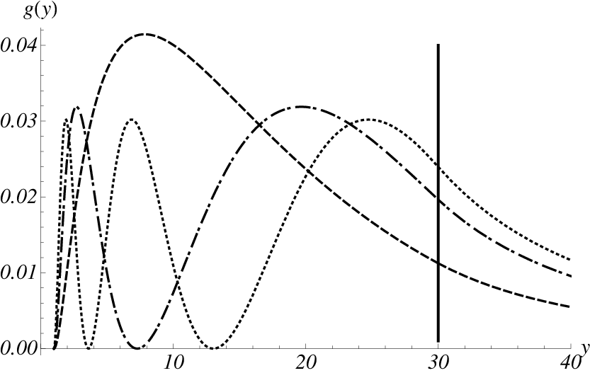
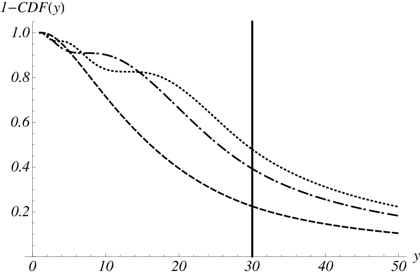
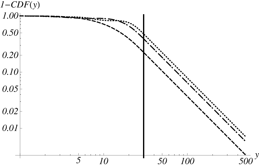
Figure (1) shows Eq. (24), the PDF $g(y)=q(y)^{2}$ and the complementary cumulative distribution function (CDF). Function $g(y)$ is plotted in its $3$ first eigenstates.

IV Dissipative term

Real systems, particularly social systems, are often conceived as open which means they exchange matter, energy or information with their surroundings. In this sense, a dissipative term $H(q^{\prime}(y),y)$ is proposed:

H(q^{\prime}(y),y)=\beta\frac{q^{\prime}(y)}{y}.

(25)

Coefficient $\beta$ will be the strength of the dissipation. This term is constructed by analogy with the Schrödinger equation in quantum mechanics, as shown in appendix B.

Using this dissipative term, the equation of motion becomes

4q^{\prime\prime}(y)+\frac{\kappa}{t(y)^{2}}\frac{q(y)}{y^{2}}=\beta\frac{q^{\prime}(y)}{y}.

(26)

The solutions $q_{1}(y)$ and $q_{2}(y)$ now have the general form

q_{i}(y)=c_{i,1}y^{\lambda+k_{i}}+c_{i,2}y^{\lambda-k_{i}},

(27)

where $c_{i,1}$ and $c_{i,2}$ are integration constants, and coefficient $k_{i}$ obeys

k_{i}=\sqrt{\lambda^{2}-\frac{\kappa}{4t_{i}^{2}}},

(28)

with

\lambda=\frac{4-\beta}{8}.

(29)

Using the same conditions as in section (III), a particular solution can be written as

q(y)=\left\{\begin{array}[]{lcl}c_{1\,}y^{\lambda}\sin(k_{1}\log(y)),&&1\leq y\leq y_{0}\\ c_{2}\,y^{\lambda-k_{2}},&&y>y_{0}\end{array}\right..

(30)

The scaling parameter $\alpha_{tail}$ of the Pareto distribution can now be written in terms of the system characteristics and a dissipative term

\alpha_{tail}=2\left(k_{2}-\lambda\right)-1.

(31)

Using Eqs. (29) and (31) it can be inferred the information exchange direction with the surroundings: if $\lambda<1/2$ the system gain information, if $\lambda>1/2$ the system loose information and if $\lambda=1/2$ the system is in equilibrium with the environment. In natural systems a direct equivalence with entropy changes can be made using Fisher information as an entropy measure [17].

V application of the model

This model can be used in a bottom-up approach, because the macroscopic parameters of an observed distribution, such as the scaling parameter and the $y_{min}$ value, can be related or explained using the microscopic parameters $t_{1}$ , $t_{2}$ , $\kappa$ and $y_{0}$ using Eq. (19). This model can also be seen in a top-down approach, because it can be used to fit an observed PDF by means of numerical estimation of parameters.

To fit an observed PDF, the scaling parameter $\alpha_{tail}$ and the $y_{min}$ value can be estimated using the maximum likelihood (ML) method as standard [27]. Then, using the corresponding relation equation derived from the normalization condition e.g. Eqs. (22) and (23), several eigenvalues $k_{1}$ can be computed to describe the head. Because there could be several different values for $k_{1}$ , the head can be fitted using a linear combination of eigenvalues.

In both approaches the model allows the interpretation of the parameters in terms of physical quantities or properties of the system. In this sense the model is not only descriptive but might become useful to control the system. By employing equations (28) and (31) the scaling parameter of the tail can be adjusted, and the shape of the head can be restricted to some particular values.

Finally, it is apparent that this model was derived using a piecewise function $t(y)$ Eq. (8), with only two pieces; but the solution can be generalized to $n$ pieces. In this case the solution will be a piecewise solution with $n$ different $q_{i}(y)$ . A PDF with several scale parameters in the tail can be useful if the observed PDF shows more than one slope in the upper-tail.

V.1 Fitting the real data set

The model was used to fit $4$ data sets with power law tails. The power law tails of selected data set were studied in [27, 1] (downloaded from http://tuvalu.santafe.edu/~aaronc/powerlaws/data.htm) and in [12], where world wealth distribution is simulated using an agent based model (ABM).

To fit the whole PDF, first the scaling parameter $\alpha_{tail}$ and the $y_{min}$ were estimated using an ML method, then the strength of the dissipative term and the shape of the head (a linear combination of the first two eigenstates) were estimated by direct minimization of the Kolmogorov-Smirnov statistic.

The data set comprised:

1.

The numbers of customers affected by electrical blackouts in the United States between 1984 and 2002 ( $211$ registers).
2.

The human population of US cities in the 2000 US Census ( $19447$ registers).
3.

Peak gamma-ray intensity of solar flares between 1980 and 1989 ( $12773$ registers).
4.

World wealth distribution simulated using an ABM ( $5000$ agents).

Table (1) shows boundary conditions and estimated parameters. Figure (2) shows fitted distributions. Plots were made in a linear plane to observe the fit of the head and in a Log-Log plane to observed the fit of the tail.

Data set	$t(y)$	$y_{min}$	$\alpha_{tail}$	$\lambda$	Information flow	$k_{1}$	$D_{KL}$	$D_{C}$
1	One step	$228000$	$1.2(1)$	$-0.1$	In	$\left(0.23,\,0.46\right)$	$0.04$	$0.11$
2	Two steps	$50580$	$1.36(5)$	$0.2$	In	$0.41$	$0.0099$	$0.011$
3	Two steps	$321$	$0.77(2)$	$2.0$	Out	$0.72$	$0.0140$	$0.0144$
4	One step	$614$	$1.68(5)$	$0.25$	In	$\left(0.44,\,0.89\right)$	$0.007$	$0.023$

Table 1: Boundaries conditions and estimated parameters for each data set. The one step function is a

2

piecewise function as in Eq. (8); the two steps functions are a

3

piecewise function. The presence of two values for the

k_{1}

parameter means that the fit of the head was made with the two first eigenstates.

D_{KL}

is the Kolmogorov-Smirnov statistic measured as the maximum difference between the observed CDF and the analytical CDF.

D_{C}=1.627/\sqrt{n}

is the Kolmogorov-Smirnov goodness-of-fit test critical statistic, from which the model is rejected, so it is necessary that

D_{KL}<D_{C}

(where

n

is the data length).

VI Discussion

In the study of data set probability distribution functions, two basic filters are usually applied. One of these involves discarding the extreme and rare events. These events are considered to be outliers because they do not seem to follow the general tendency. Indeed, using Gaussian statistics it can be seen that extreme events make the variance too wide and the results less significant [28, 29]. As a result, the tail is excluded from the analysis. Another frequently used filter discards the events of the head, because the main issue is the power law tail study. The study of power law tails is an interesting research area because properties such as self-organized criticality and scale-free can be ascribed to the system [30, 31, 32]. In this kind of study, frequent events are excluded by means of a threshold value that renders the power law tail plausible.

In this paper a model is presented that describes the whole distribution, involving the head and the distribution tail, and no data is discarded. Moreover, a relation between the scaling parameter of the power law tail and the shape of the general tendency of the head is also derived.

The model constructed becomes interesting for the study of many systems that exhibit power law tails, because it proposes an equation of motion that describes the behavior of the system and allows its parameters to be interpreted. Even if the model has a piecewise restriction function Eq. (8) it can be used to explain and fit several systems, in particular social systems. A lot of social variables, such as prices, taxes, incentives, budgets, etc., follow piecewise restrictions. The model can also be used to gain insight concerning microscopic processes in natural systems that follow power law tails and are not already well understood

The analysis and fitting of power law tails is an active research area. The computation of the scaling parameter of the PDF and the $y_{min}$ value (value from where the power law is plausible) is not as trivial as it seems [27]. The model developed here contributes to this research area: first, by taking into account all the registers in the data set; second, by offering a new interpretation of the scaling parameter and third, by providing a relation between the tail and the head.

A dissipative term was introduced into the model. This term permits the description of a large number of phenomena, and it should be interpreted in terms of the particular scenario of the system under study. For now, a simple interpretation is given in terms of the flow direction of the dissipation. A gain of information can be interpreted, as order is been established on the system, i.e. data sets $1$ , $2$ and $4$ ; a loss of information can be interpreted as the system seeking its thermodynamic equilibrium state, i.e. data set $3$ .

VII Conclusions

Using EPI theory according to the basic information principle, the equation of motion and the system PDF with a power law tail are deduced. The calculated PDF is as useful in describing the tail as the head of the PDF. In particular, the head is described as a combination of several eigenstates. This model, in a bottom-up approach, gives an explanation of the macroscopic parameters, $\alpha_{tail}$ and $y_{min}$ , and the shape of the head, from the microscopic parameters of the system. In a top-down approach the model is equally useful in fitting the tail as the head of an observed PDF, giving an interpretation for the estimated parameters.

The principal contribution of this paper to the analysis of systems with power law tail behavior concerns the relation between rare events in the tail and frequent events in head. In the literature, no one denies that there must be a relation between the head and the tail; here, a relation is proposed, by means of eigenstates. With this model it is not necessary to filter the data set and discard events: it is possible to study the general behavior in the head and take into account that the system presents complex characteristics as a power law in the tail.

Not only will the proposed dissipative term give a better fit in a top-down approach, but it permits a description to be made of the interactions between the systems and their surroundings. Using this model the scaling parameter in the tail could be understood as a combination of the structure and properties of a system and its interaction with the environment.

We believe that our model is capable of taking into account the fact that in many systems behavior is a mixture of order and disorder. It is also possible to gain insights regarding the plausible causes of emergent behavior, given the way parameters are fed into the model.

Appendix A Bounded Information

To write the information functional

\mathcal{F}=\int dy\,\frac{g^{\prime}(y)^{2}}{g(y)}-\kappa\int dz\,\frac{h^{\prime}(z)^{2}}{h(z)},

(32)

in terms of $g^{\prime}(y)$ , $g(y)$ and $y$ , the term

I^{(z)}=\int dz\,\frac{h^{\prime}(z)^{2}}{h(z)},

(33)

must be re-written.

The conservation of the probability is applied, using Eq. (7) and (8). Supposing that $y$ and $t(y)$ are random variables the PDF $h(z)$ can be written as the product of two random variables; by definition

\displaystyle h(z=t(y)\,y)

\displaystyle=

\displaystyle\int dy\,\frac{1}{|y|}g(y)p(\frac{z}{y}|y),

(34)

where the function $p(t|y)$ is the probability of $t=t_{1}$ or $t=t_{2}$ , given $y$ . This probability function, $p(t|y)$ , can be written in term of the delta function $\delta(y-y_{0})$ and the Heaviside function $H(y-y_{0})$ as

	$\displaystyle p(t\|y)$	$\displaystyle=$	$\displaystyle a_{1}\delta(t-t_{1})(1-H(y-y_{0})$		(35)
			$\displaystyle+a_{2}\delta(t-t_{2})H(y-y_{0}),$		(35)

where $a_{1}+a_{2}=1$ .

Using equations Eq. (35) in Eq. (34) we get

	$\displaystyle h(z)$	$\displaystyle=$	$\displaystyle\intop_{0}^{\infty}dy\,\frac{1}{\|y\|}g(y)\left\{a_{1}\delta(\frac{z}{y}-t_{1})(1-H(y-y_{0})+a_{2}\delta(\frac{z}{y}-t_{2})H(y-y_{0})\right\}$		(36)
		$\displaystyle=$	$\displaystyle\intop_{0}^{y_{0}}dy\,\frac{1}{\|y\|}g(y)a_{1}\delta(\frac{z}{y}-t_{1})+\intop_{y_{0}}^{\infty}dy\,\frac{1}{\|y\|}g(y)a_{2}\delta(\frac{z}{y}-t_{2}).$		(36)

Now $h^{\prime}(y)$ is calculated taken the derivative $\frac{\partial}{\partial y}$ of Eq. (36),

$\displaystyle\frac{\partial h(z)}{\partial z}$	$\displaystyle=$	$\displaystyle\intop_{0}^{y0}dy\,\frac{1}{\|y\|}g(y)a_{1}\,\frac{\partial}{\partial z}\delta(\frac{z}{y}-t_{1})+\intop_{y_{0}}^{\infty}dy\,\frac{1}{\|y\|}g(y)a_{2}\,\frac{\partial}{\partial z}\delta(\frac{z}{y}-t_{2})$	(37)
	$\displaystyle=$	$\displaystyle-\intop_{0}^{y0}dy\,\frac{1}{\|y\|}g(y)a_{1}\,\frac{\left\|y\right\|}{z}\delta(z-t_{1}y)-\intop_{y_{0}}^{\infty}dy\,\frac{1}{\|y\|}g(y)a_{2}\,\frac{\left\|y\right\|}{z}\delta(z-t_{2}y)$
	$\displaystyle=$	$\displaystyle-\frac{1}{z}h(z).$

This last development takes into account that $g(\frac{z}{t_{i}})=t_{i}h(z)$ .

Finally, using Eqs. (37) and (7), we write $I^{(z)}=\int dz\,\frac{h^{\prime}(z)^{2}}{h(z)}$ as

$\displaystyle I^{(z)}$	$\displaystyle=$	$\displaystyle\int dz\,\frac{h(z)}{z^{2}}$	(38)
	$\displaystyle=$	$\displaystyle\intop_{1}^{z^{}}dz\,\frac{h(z)}{z^{2}}+\intop_{z*}^{\infty}dz\,\frac{h(z)}{z^{2}}$
	$\displaystyle=$	$\displaystyle\intop_{1}^{y_{0}}dy\,t_{1}\frac{h(t_{1}y)}{t_{1}^{2}y^{2}}+\intop_{y_{0}}^{\infty}dy\,t_{2}\frac{h(t_{2}y)}{t_{2}^{2}y^{2}}$
	$\displaystyle=$	$\displaystyle\int dy\,\frac{1}{t(y)^{2}}\frac{g(y)}{y^{2}},$

where $z*=t_{1}y_{0}$ and $z**=t_{2}y_{0}$ , and $h(t_{i}y)=\frac{1}{t_{i}}g(y)$ .

Appendix B Dissipative term

To introduce a dissipative term into the analysis it is only necessary to equate the second order differential equation Eq. (16) to a function $H(q^{\prime}(y),y)$ , where $H(q^{\prime}(y),y)$ has a general form of a dissipative term, that is, in terms of $q^{\prime}(y)$ . Here, a particular form for the dissipative term is inspired by the mathematical equivalence of Eq (16) with the Schrödinger equation. Under the change of variable $\tilde{y}=\log\,y$ , the Schrödinger equation of a free particle

a\varphi^{\prime\prime}(\tilde{y})+b\varphi(\tilde{y})=0,

(39)

becomes

aq^{\prime\prime}(y)+a\frac{q^{\prime}(y)}{y}+b\frac{q(y)}{y^{2}}=0.

(40)

In the same way, the general solution of the Schrödinger equation

\varphi(\tilde{y})=A\exp\left(k\tilde{y}\right)+B\exp\left(-k\tilde{y}\right),

(41)

becomes

q(y)=A\,y^{k}+B\,y^{-k}.

(42)

In both cases, $k=\pm\sqrt{-b/a}$ .

Comparing Eq. (40) with Eq. (16) an additional term $a\frac{q^{\prime}(y)}{y}$ can be identified. Because this term has a first derivative, by analogy with dissipative forces we propose that $a\frac{q^{\prime}(y)}{y}$ can be related to a dissipative source of information. So, by analogy with a quantum system we propose

H(q^{\prime}(y),y)=\beta\frac{q^{\prime}(y)}{y},

(43)

where, $\beta$ is a constant, related to the strength of the dissipation.

The dissipative term is still not well understood, but allows a sharp estimate to be made of the scaling parameter at the tail: see Eq. (30). It is also interesting to discuss a new interpretation for the scaling parameter of the power law tail using Eq. (31).

Acknowledgements.

We acknowledge COLCIENCIAS’s financial support R.B, and the Research Fund of the Engineering Faculty of the Universidad de los Andes, Colombia R.Z..

References

[1] M. E. J. Newman, Contemporary Physics 46, 323 (2005)
[2] P. Andriani and B. McKelvey, Organization Science 20, 1053 (2009)
[3] B. Mandelbrot, in Communication Theory, edited by B. W. Jackson (1953) pp. 486–502
[4] P. Bak, C. Tang, and K. Wiesenfeld, Phys. Rev. Lett. 59, 381 (1987)
[5] S. Abe and A. Rajagopal, J. Phys. A: Math. Theor. 33 (2000)
[6] C. B. Yang, J. Phys. A: Math. Theor. 37, L523 (2004)
[7] F. Pennini and A. Plastino, Physica A 334, 132 (2004)
[8] A. L. Barabási, H. Jeong, Z. Neda, E. Ravasz, A. Schubert, and T. Vicsek, Physica A 311, 590 (2002)
[9] M. Mitzenmacher, Internet Mathematics 1, 305 (2002)
[10] J. C. Bohorquez, S. Gourley, A. R. Dixon, M. Spagat, and N. F. Johnson, Nature 462, 911 (2009)
[11] W. J. Reed, Physica A 319, 469 (2003)
[12] N. Lammoglia, V. Munoz, J. Rogan, B. Toledo, R. Zarama, and J. A. Valdivia, Phys. Rev. E 78, 047103 (2008)
[13] J. M. Sarabia and F. Prieto, Physica A 388, 4179 (2009)
[14] B. R. Frieden, Science from Fisher Information: A Unification (Cambridge University Press, 2004)
[15] B. R. Frieden, Phys. Rev. A 41, 4265 (1990)
[16] B. R. Frieden and W. J. Cocke, Phys. Rev. E 54, 257 (1996)
[17] B. R. Frieden and B. H. Soffer, Phys. Rev. E 52, 2274 (1995)
[18] B. R. Frieden, A. Plastino, A. R. Plastino, and B. H. Soffer, Phys. Rev. E 60, 48 (1999)
[19] P. M. Binder, Phys. Rev. E 61, R3303 (2000)
[20] R. A. Gatenby and B. R. Frieden, Cancer Research 62, 3675 (2002)
[21] R. J. Hawkins and B. R. Frieden, Physics Letters A 322, 126 (2004)
[22] B. R. Frieden and R. A. Gatenby, Phys. Rev. E 72 (2005)
[23] R. Gatenby and B. R. Frieden, Bulletin of Mathematical Biology 69, 635 (2007)
[24] R. J. Hawkins, M. Aoki, and B. R. Frieden, Physica A 389, 3565 (2010)
[25] R. A. Fisher, Philos. Trans. R. Soc. London Series A 222, 309 (1922)
[26] R. A. Fisher, Mathematical Proceedings of the Cambridge Philosophical Society 22, 700 (1925)
[27] A. Clauset, C. Shalizi, and M. Newman, SIAM Review 51, 661 (2009)
[28] R. M. Sakia, Statistician 41, 169 (1992)
[29] T.-C. Cheng, Comput. Stat. Data An. 49, 875 (2005)
[30] A. L. Barabási and R. Albert, Science 286, 509 (1999)
[31] D. Sornette, Critical Phenomena in Natural Sciences: Chaos, Fractals, Selforganization and Disorder: Concepts and Tools (Springer, 2006)
[32] M. Mitzenmacher, Internet Mathematics 1, 226 (2003)