跳到论文正文
W Papers独立论文阅读器 arXiv:1102.5259 论文正文 计算阅读时间 · 0%
引用这篇论文根据当前论文元数据生成,正式投稿前建议核对。


License: arXiv.org perpetual non-exclusive license
arXiv:1102.5259v1 [math-ph] 25 Feb 2011

Dirichlet-to-Neumann and Neumann-to-Dirichlet methods for bound states of the Helmholtz equation

Sebastian Bielski Affiliation: Atomic Physics Division, Department of Atomic Physics and Luminescence, Affiliation: Faculty of Applied Physics and Mathematics, Gdańsk University of Technology, Affiliation: Narutowicza 11/12, PL 80–233 Gdańsk, Poland Email: Email:bolo@mif.pg.gda.pl
August 24, 2026
Abstract

Two methods for computing bound states of the Helmholtz equation in a finite domain are presented. The methods are formulated in terms of the Dirichlet-to-Neumann (DtN) and Neumann-to-Dirichlet (NtD) surface integral operators. They are adapted from the DtN and NtD methods for bound states of the Schrödinger equation in ℝ3\mathbb{R}^{3}. A variational principle that enables the usage of the operators is constructed. The variational principle allows the use of discontinuous (in values or derivatives) trial functions. A numerical example presenting the usefulness of the DtN and NtD methods is given.

1 Introduction

In this work we are interested in finding solutions to the problem consisting of the Helmholtz equation defined in a two- (or more) dimensional finite volume Γ\Gamma:

Δ​Ψ​(𝐫)+k2​Ψ​(𝐫)=0,𝐫∈Γ\Delta\Psi(\mathbf{r})+k^{2}\Psi(\mathbf{r})=0,\qquad\mathbf{r}\in\Gamma (1)

and the homogeneous Dirichlet condition on the boundary ∂Γ\partial\Gamma:

Ψ⁡(𝐫)=0,𝐫∈∂Γ.\Psi(\mathbf{r})=0,\qquad\mathbf{r}\in\partial\Gamma. (2)

The set (1)–(2) is an eigenproblem in which the values {−k2}\left\{-k^{2}\right\} are the eigenvalues and {Ψ}\left\{\Psi\right\} are the corresponding eigenfunctions. The eigenproblem (1)–(2) appears in many different areas of physics. It describes, for example, the behaviour of a particle confined in an infinitely deep potential (in this case k2k^{2} is proportional to the energy of the particle while |Ψ|2\left|\Psi\right|^{2} is the probability density) or vibrations of a homogeneous membrane (kk is proportional to the vibration frequency, Ψ\Psi is the amplitude), it is useful in studying the propagation of electromagnetic waves in waveguides, etc. So, although the problem of finding eigenvalues and eigenfunctions of the Laplace operator has been known for many decades, it remains very important in many fields.

The standard analytical approach to problems like (1)–(2) is the method of separation of variables. The first step in the method is to choose an appropriate coordinate system. The choice depends on the shape of ∂Γ\partial\Gamma. In practice, only in some cases it is possible to find a system fitted to the geometry of a problem and to obtain the exact solutions using the separation of variables technique. In general, the shape of the boundary of Γ\Gamma may be arbitrary and no useful coordinate system may be found, so other methods may need to be used. There are many different attempts. Amore [1] has applied a collocation method using so-called little sinc functions for problems defined in two-dimensional domains of arbitrary shape. Chakraborty et al. [2] have presented an analytical perturbative method. In the two mentioned works brief surveys of other methods may be found. Recently, Steinbach et al. [3] have formulated a boundary element domain decomposition method that enables to transform the original problem to a new one defined on the boundaries separating the subdomains.

The goal of this work is to present two methods that are applicable to the eigenproblem (1)–(2) in case the domain is such that it can be naturally divided into two non-overlapping subdomains. The methods consist in the application of a variational principle allowing the use of trial functions that may experience jumps in values or derivatives when passing from one subdomain to other. The Dirichlet-to-Neumann (DtN) integral operator or the Neumann-to-Dirichlet (NtD) integral operator is used, both are defined on the interface separating the subdomains. Each of the methods allows to replace the initial problem (1)–(2) with a new problem defined in one of the subdomains and on the interface. The methods are related to the DtN and the NtD embedding methods for the bound states of the Schrödinger equation (defined in ℝ3\mathbb{R}^{3}) and their relativistic counterparts [4, 5]. The DtN method for the Schrödinger equation is a close relative of the embedding method proposed by Inglesfield [6]. In the Inglesfield’s method the Green function formalism is used while in the DtN (and NtD) method an operator approach analogous to that employed in the R-matrix theory [7, 8] is applied.

The structure of the paper is as follows. In section II a systematic construction of a variational principle (allowing the use of discontinuous trial functions) for bound states of the Helmholtz equation is presented. In section III the DtN and NtD operators are defined. Sections IV and V are devoted to the formalism of the DtN and NtD methods for bound states of the Helmholtz equation. In section VI a numerical example is provided.

2 Variational principle allowing the use of discontinuous trial functions

Let Γ\Gamma be a two- (or more) dimensional finite domain of such a shape that it may be in a natural way divided into two subdomains, ΓI\Gamma_{I} and ΓI​I\Gamma_{II}, separated by a smooth curve (or surface) denoted by 𝒮\mathcal{S}, as shown in figure 1. Thus, the boundary of ΓI\Gamma_{I} consists of ∂ΓI\partial\Gamma_{I} and 𝒮\mathcal{S} while the boundary of ΓI​I\Gamma_{II} is composed of ∂ΓI​I\partial\Gamma_{II} and 𝒮\mathcal{S}.

Refer to caption
Figure 1: Partitioning of the domain Γ\Gamma into two subdomains ΓI\Gamma_{I} and ΓI​I\Gamma_{II}, separated by the interface 𝒮\mathcal{S}; 𝐧⁡(𝝆)\mathbf{n}(\boldsymbol{\rho}) is the unit vector normal to the interface 𝒮\mathcal{S} at the point 𝝆\boldsymbol{\rho}.

A position vector lying on 𝒮\mathcal{S} will be denoted by 𝝆\boldsymbol{\rho} and 𝐧⁡(𝝆)\mathbf{n}(\boldsymbol{\rho}) will be the unit vector normal to 𝒮\mathcal{S} at the point 𝝆\boldsymbol{\rho} (we assume that 𝐧⁡(𝝆)\mathbf{n}(\boldsymbol{\rho}) is always pointed outward from ΓI\Gamma_{I}). Denoting

Ψi​(𝐫)=Ψ⁡(𝐫)(𝐫∈Γi,i=I,II),\Psi_{i}(\mathbf{r})=\Psi(\mathbf{r})\qquad(\mathbf{r}\in\Gamma_{i}\,;i=I,\textit{II}), (3)

we may rewrite the initial problem (1)–(2) as

Δ​ΨI​(𝐫)+k2​ΨI​(𝐫)=0,𝐫∈ΓI,\Delta\Psi_{I}(\mathbf{r})+k^{2}\Psi_{I}(\mathbf{r})=0,\qquad\mathbf{r}\in\Gamma_{I}, (4)
ΨI​(𝐫)=0,𝐫∈∂ΓI,\Psi_{I}(\mathbf{r})=0,\qquad\mathbf{r}\in\partial\Gamma_{I}, (5)
Δ​ΨI​I​(𝐫)+k2​ΨI​I​(𝐫)=0,𝐫∈ΓI​I,\Delta\Psi_{II}(\mathbf{r})+k^{2}\Psi_{II}(\mathbf{r})=0,\qquad\mathbf{r}\in\Gamma_{II}, (6)
ΨI​I​(𝐫)=0,𝐫∈∂ΓI​I.\Psi_{II}(\mathbf{r})=0,\qquad\mathbf{r}\in\partial\Gamma_{II}. (7)

The function Ψ⁡(𝐫)\Psi(\mathbf{r}) and its gradient must be continuous in the whole domain Γ\Gamma, so it is obvious that the functions ΨI​(𝐫)\Psi_{I}(\mathbf{r}) and ΨI​I​(𝐫)\Psi_{II}(\mathbf{r}) obey the equations:

ΨI​(𝝆)−ΨI​I​(𝝆)=0,\Psi_{I}(\boldsymbol{\rho})-\Psi_{II}(\boldsymbol{\rho})=0, (8)
∇⟂ΨI​(𝝆)−∇⟂ΨI​I​(𝝆)=0,\nabla_{\perp}\Psi_{I}(\boldsymbol{\rho})-\nabla_{\perp}\Psi_{II}(\boldsymbol{\rho})=0, (9)

where

∇⟂Ψi​(𝝆)=𝐧⁡(𝝆)⋅∇Ψi​(𝐫)|𝐫=𝝆\nabla_{\perp}\Psi_{i}(\boldsymbol{\rho})=\mathbf{n}(\boldsymbol{\rho})\cdot\boldsymbol{\nabla}\Psi_{i}(\mathbf{r})\Big|_{\mathbf{r}=\boldsymbol{\rho}} (10)

is the normal derivative of Ψi\Psi_{i} at 𝝆\boldsymbol{\rho}.

We want to determine the values of {k2}\left\{k^{2}\right\} and the corresponding functions {Ψ⁡(𝐫)}\left\{\Psi(\mathbf{r})\right\}. Basing on equations (4), (6), (8) and (9) and using a method proposed by Gerjuoy et al. [9] we define a functional that provides some estimate of one of the sought values {k2}\left\{k^{2}\right\}:

ℱ[k¯,Ψ¯I,Ψ¯I​I;Λ¯I,Λ¯I​I,λ¯,χ¯]=k¯2+⟨Λ¯I|[Δ+k¯2]Ψ¯I⟩I+⟨Λ¯I​I|[Δ+k¯2]Ψ¯I​I⟩I​I\displaystyle\mathcal{F}[\overline{k},\overline{\Psi}_{I},\overline{\Psi}_{II};\overline{\Lambda}_{I},\overline{\Lambda}_{II},\overline{\lambda},\overline{\chi}]=\overline{k}\,^{2}+\big<\overline{\Lambda}_{I}\big|[\Delta+\overline{k}\,^{2}]\overline{\Psi}_{I}\big>_{I}+\big<\overline{\Lambda}_{II}\big|[\Delta+\overline{k}\,^{2}]\overline{\Psi}_{II}\big>_{II}
+(λ¯|Ψ¯I−Ψ¯I​I)+(χ¯|∇⟂Ψ¯I−∇⟂Ψ¯I​I).\displaystyle\qquad+\big(\overline{\lambda}\big|\overline{\Psi}_{I}-\overline{\Psi}_{II}\big)+\big(\overline{\chi}\big|\nabla_{\perp}\overline{\Psi}_{I}-\nabla_{\perp}\overline{\Psi}_{II}\big). (11)

The scalar products are defined as follows:

⟨Φ|Φ′⟩i=∫Γid𝐫Φ∗(𝐫)Φ′(𝐫),\big<\Phi\big|\Phi^{\prime}\big>_{i}=\int_{\Gamma_{i}}\mathrm{d}\mathbf{r}\>\Phi^{*}(\mathbf{r})\Phi^{\prime}(\mathbf{r}), (12)
(Φ|Φ′)=∫𝒮d​𝝆​Φ∗​(𝝆)​Φ′​(𝝆)\big(\Phi\big|\Phi^{\prime}\big)=\int_{\mathcal{S}}\mathrm{d}\boldsymbol{\rho}\>\Phi^{*}(\boldsymbol{\rho})\Phi^{\prime}(\boldsymbol{\rho}) (13)

(d​𝐫\mathrm{d}\mathbf{r} is an infinitesimal volume element around the point 𝐫\mathbf{r}, d​𝝆\mathrm{d}\boldsymbol{\rho} is an infinitesimal scalar element of the interface 𝒮\mathcal{S} around the point 𝝆\boldsymbol{\rho}, and ∗* denotes the complex conjugation). The value k¯\overline{k}, the function Ψ¯I\overline{\Psi}_{I} (vanishing on ∂ΓI\partial\Gamma_{I}) and the function Ψ¯I​I\overline{\Psi}_{II} (vanishing on ∂ΓI​I\partial\Gamma_{II}) are some trial estimates of the exact quantities kk, ΨI\Psi_{I} and ΨI​I\Psi_{II}. The functions Λ¯I\overline{\Lambda}_{I} (defined in ΓI\Gamma_{I}), Λ¯I​I\overline{\Lambda}_{II} (defined in ΓI​I\Gamma_{II}), λ¯\overline{\lambda} and χ¯\overline{\chi} (both defined on 𝒮\mathcal{S}) play role of the Lagrange functions including equations (4), (6), (8) and (9) in the functional. The first variation of the functional (11) with respect to arbitrary variations of k¯\overline{k}, Ψ¯I\overline{\Psi}_{I}, Ψ¯I​I\overline{\Psi}_{II} about kk, ΨI\Psi_{I}, ΨI​I\Psi_{II} (supposing that the variations δ​ΨI\delta\Psi_{I} and δ​ΨI​I\delta\Psi_{II} vanish on ∂ΓI\partial\Gamma_{I} and ∂ΓI​I\partial\Gamma_{II}, respectively) and Λ¯I\overline{\Lambda}_{I}, Λ¯I​I\overline{\Lambda}_{II}, λ¯\overline{\lambda}, χ¯\overline{\chi} about some arbitrarily chosen ΛI\Lambda_{I}, ΛI​I\Lambda_{II}, λ\lambda, χ\chi may be written as

δℱ[k,ΨI,ΨI​I;ΛI,ΛI​I,λ,χ]=2kδk[1+⟨ΛI|ΨI⟩I+⟨ΛI​I|ΨI​I⟩I​I]\displaystyle\delta\mathcal{F}[k,\Psi_{I},\Psi_{II};\Lambda_{I},\Lambda_{II},\lambda,\chi]=2k\delta k\left[1+\big<\Lambda_{I}\big|\Psi_{I}\big>_{I}+\big<\Lambda_{II}\big|\Psi_{II}\big>_{II}\right]
+⟨[Δ+k2]ΛI|δΨI⟩I+⟨[Δ+k2]ΛI​I|δΨI​I⟩I​I\displaystyle\qquad+\big<[\Delta+k^{2}]\Lambda_{I}\big|\delta\Psi_{I}\big>_{I}+\big<[\Delta+k^{2}]\Lambda_{II}\big|\delta\Psi_{II}\big>_{II}
+(λ−∇⟂ΛI|δ​ΨI)−(λ−∇⟂ΛI​I|δ​ΨI​I)\displaystyle\qquad+\big(\lambda-\nabla_{\perp}\Lambda_{I}\big|\delta\Psi_{I}\big)-\big(\lambda-\nabla_{\perp}\Lambda_{II}\big|\delta\Psi_{II}\big)
+(χ+ΛI|∇⟂δ​ΨI)−(χ+ΛI​I|∇⟂δ​ΨI​I)\displaystyle\qquad+\big(\chi+\Lambda_{I}\big|\nabla_{\perp}\delta\Psi_{I}\big)-\big(\chi+\Lambda_{II}\big|\nabla_{\perp}\delta\Psi_{II}\big)
+(ΛI|∇⟂δ​ΨI)I+(ΛI​I|∇⟂δ​ΨI​I)I​I,\displaystyle\qquad+\big(\Lambda_{I}\big|\nabla_{\perp}\delta\Psi_{I}\big)_{I}+\big(\Lambda_{II}\big|\nabla_{\perp}\delta\Psi_{II}\big)_{II}, (14)

where

(Φ|Φ′)i=∫∂Γid​𝐫​Φ∗​(𝐫)​Φ′​(𝐫).\big(\Phi\big|\Phi^{\prime}\big)_{i}=\int_{\partial\Gamma_{i}}\mathrm{d}\mathbf{r}\>\Phi^{*}(\mathbf{r})\Phi^{\prime}(\mathbf{r}). (15)

In the above scalar product, d​𝐫\mathrm{d}\mathbf{r} is an infinitesimal scalar element of ∂Γi\partial\Gamma_{i} around the point 𝐫\mathbf{r} (cf. the definitions (12) and (13)). We seek such functions ΛI\Lambda_{I}, ΛI​I\Lambda_{II}, λ\lambda and χ\chi for which the functional is stationary, i.e. its first variation is equal to zero. So the functions ΛI\Lambda_{I}, ΛI​I\Lambda_{II}, λ\lambda and χ\chi fulfil the equations:

1+⟨ΛI|ΨI⟩I+⟨ΛI​I|ΨI​I⟩I​I=0,1+\big<\Lambda_{I}\big|\Psi_{I}\big>_{I}+\big<\Lambda_{II}\big|\Psi_{II}\big>_{II}=0, (16)
[Δ+k2]​Λi​(𝐫)=0,𝐫∈Γi,[\Delta+k^{2}]\Lambda_{i}(\mathbf{r})=0,\qquad\mathbf{r}\in\Gamma_{i}, (17)
Λi​(𝐫)=0,𝐫∈∂Γi,\Lambda_{i}(\mathbf{r})=0,\qquad\mathbf{r}\in\partial\Gamma_{i}, (18)
λ⁡(𝝆)−∇⟂Λi​(𝝆)=0,\lambda(\boldsymbol{\rho})-\nabla_{\perp}\Lambda_{i}(\boldsymbol{\rho})=0, (19)
χ⁡(𝝆)+Λi​(𝝆)=0,\chi(\boldsymbol{\rho})+\Lambda_{i}(\boldsymbol{\rho})=0, (20)

where i=I,IIi=I,\textit{II}. From equations (19) and (20) we obtain

ΛI​(𝝆)−ΛI​I​(𝝆)=0,\Lambda_{I}(\boldsymbol{\rho})-\Lambda_{II}(\boldsymbol{\rho})=0, (21)
∇⟂ΛI​(𝝆)−∇⟂ΛI​I​(𝝆)=0.\nabla_{\perp}\Lambda_{I}(\boldsymbol{\rho})-\nabla_{\perp}\Lambda_{II}(\boldsymbol{\rho})=0. (22)

Comparying equations (17), (18), (21) and (22) with equations (4)–(9) we find that ΛI​(𝐫)\Lambda_{I}(\mathbf{r}) and ΛI​I​(𝐫)\Lambda_{II}(\mathbf{r}) obey the same differential equations and the same boundary conditions as ΨI​(𝐫)\Psi_{I}(\mathbf{r}) and ΨI​I​(𝐫)\Psi_{II}(\mathbf{r}). This means that the functions ΛI\Lambda_{I} and ΛI​I\Lambda_{II} are proportional to ΨI\Psi_{I} and ΨI​I\Psi_{II}:

Λi​(𝐫)=η​Ψi​(𝐫)(i=I,II).\Lambda_{i}(\mathbf{r})=\eta\Psi_{i}(\mathbf{r})\qquad(i=I,\textit{II}). (23)

The value of η\eta may be found using the formulas (23) in equation (16):

η=−1⟨ΨI|ΨI⟩I+⟨ΨI​I|ΨI​I⟩I​I.\eta=-\frac{1}{\big<\Psi_{I}\big|\Psi_{I}\big>_{I}+\big<\Psi_{II}\big|\Psi_{II}\big>_{II}}. (24)

According to equations (19), (20) and (23), we may write

λ⁡(𝝆)=η⁡[a​∇⟂ΨI​(𝝆)+(1−a)​∇⟂ΨI​I​(𝝆)],\lambda(\boldsymbol{\rho})=\eta[a\nabla_{\perp}\Psi_{I}(\boldsymbol{\rho})+(1-a)\nabla_{\perp}\Psi_{II}(\boldsymbol{\rho})], (25)
χ⁡(𝝆)=−η⁡[b​ΨI​(𝝆)+(1−b)​ΨI​I​(𝝆)],\chi(\boldsymbol{\rho})=-\eta[b\Psi_{I}(\boldsymbol{\rho})+(1-b)\Psi_{II}(\boldsymbol{\rho})], (26)

where aa and bb are arbitrary complex constants.

Now, let us assume, that the trial Lagrange functions Λ¯I\overline{\Lambda}_{I},Λ¯I​I\overline{\Lambda}_{II},λ¯\overline{\lambda}, χ¯\overline{\chi}, appearing in the functional (11), are related to the estimates Ψ¯I\overline{\Psi}_{I} and Ψ¯I​I\overline{\Psi}_{II} in the same way that the functions ΛI\Lambda_{I}, ΛI​I\Lambda_{II}, λ\lambda, χ\chi are related to the exact functions ΨI\Psi_{I} and ΨI​I\Psi_{II}. Using the formulas obtained from equations (23)–(26) by replacing the functions ΨI\Psi_{I}, ΨI​I\Psi_{II}, ΛI\Lambda_{I}, ΛI​I\Lambda_{II}, λ\lambda and χ\chi with the trial functions Ψ¯I\overline{\Psi}_{I}, Ψ¯I​I\overline{\Psi}_{II}, Λ¯I\overline{\Lambda}_{I}, Λ¯I​I\overline{\Lambda}_{II}, λ¯\overline{\lambda} and χ¯\overline{\chi}, transforms the functional (11) to

ℱ⁡[Ψ¯I,Ψ¯I​I]=−⟨Ψ¯I|ΔΨ¯I⟩I+⟨Ψ¯I​I|ΔΨ¯I​I⟩I​I⟨Ψ¯I|Ψ¯I⟩I+⟨Ψ¯I​I|Ψ¯I​I⟩I​I−(a​∇⟂Ψ¯I+[1−a]​∇⟂Ψ¯I​I|Ψ¯I−Ψ¯I​I)⟨Ψ¯I|Ψ¯I⟩I+⟨Ψ¯I​I|Ψ¯I​I⟩I​I\displaystyle\mathcal{F}[\overline{\Psi}_{I},\overline{\Psi}_{II}]=-\frac{\big<\overline{\Psi}_{I}\big|\Delta\overline{\Psi}_{I}\big>_{I}+\big<\overline{\Psi}_{II}\big|\Delta\overline{\Psi}_{II}\big>_{II}}{\big<\overline{\Psi}_{I}\big|\overline{\Psi}_{I}\big>_{I}+\big<\overline{\Psi}_{II}\big|\overline{\Psi}_{II}\big>_{II}}-\frac{\big(a\nabla_{\perp}\overline{\Psi}_{I}+[1-a]\nabla_{\perp}\overline{\Psi}_{II}\big|\overline{\Psi}_{I}-\overline{\Psi}_{II}\big)}{\big<\overline{\Psi}_{I}\big|\overline{\Psi}_{I}\big>_{I}+\big<\overline{\Psi}_{II}\big|\overline{\Psi}_{II}\big>_{II}}
+(b​Ψ¯I+[1−b]​Ψ¯I​I|∇⟂Ψ¯I−∇⟂Ψ¯I​I)⟨Ψ¯I|Ψ¯I⟩I+⟨Ψ¯I​I|Ψ¯I​I⟩I​I.\displaystyle\qquad+\frac{\big(b\overline{\Psi}_{I}+[1-b]\overline{\Psi}_{II}\big|\nabla_{\perp}\overline{\Psi}_{I}-\nabla_{\perp}\overline{\Psi}_{II}\big)}{\big<\overline{\Psi}_{I}\big|\overline{\Psi}_{I}\big>_{I}+\big<\overline{\Psi}_{II}\big|\overline{\Psi}_{II}\big>_{II}}. (27)

Our functional is supposed to estimate of a real quantity, so it should possess the property

ℱ∗​[Ψ¯I,Ψ¯I​I]=ℱ⁡[Ψ¯I,Ψ¯I​I].\mathcal{F}^{*}[\overline{\Psi}_{I},\overline{\Psi}_{II}]=\mathcal{F}[\overline{\Psi}_{I},\overline{\Psi}_{II}]. (28)

After some rearrangements we find that equation (28) is obeyed if

b=1−a∗b=1-a^{*} (29)

and the final form of the functional is

ℱ⁡[Ψ¯I,Ψ¯I​I]=−⟨Ψ¯I|ΔΨ¯I⟩I+⟨Ψ¯I​I|ΔΨ¯I​I⟩I​I⟨Ψ¯I|Ψ¯I⟩I+⟨Ψ¯I​I|Ψ¯I​I⟩I​I−(a​∇⟂Ψ¯I+[1−a]​∇⟂Ψ¯I​I|Ψ¯I−Ψ¯I​I)⟨Ψ¯I|Ψ¯I⟩I+⟨Ψ¯I​I|Ψ¯I​I⟩I​I\displaystyle\mathcal{F}[\overline{\Psi}_{I},\overline{\Psi}_{II}]=-\frac{\big<\overline{\Psi}_{I}\big|\Delta\overline{\Psi}_{I}\big>_{I}+\big<\overline{\Psi}_{II}\big|\Delta\overline{\Psi}_{II}\big>_{II}}{\big<\overline{\Psi}_{I}\big|\overline{\Psi}_{I}\big>_{I}+\big<\overline{\Psi}_{II}\big|\overline{\Psi}_{II}\big>_{II}}-\frac{\big(a\nabla_{\perp}\overline{\Psi}_{I}+[1-a]\nabla_{\perp}\overline{\Psi}_{II}\big|\overline{\Psi}_{I}-\overline{\Psi}_{II}\big)}{\big<\overline{\Psi}_{I}\big|\overline{\Psi}_{I}\big>_{I}+\big<\overline{\Psi}_{II}\big|\overline{\Psi}_{II}\big>_{II}}
+([1−a∗]​Ψ¯I+a∗​Ψ¯I​I|∇⟂Ψ¯I−∇⟂Ψ¯I​I)⟨Ψ¯I|Ψ¯I⟩I+⟨Ψ¯I​I|Ψ¯I​I⟩I​I.\displaystyle\qquad+\frac{\big([1-a^{*}]\overline{\Psi}_{I}+a^{*}\overline{\Psi}_{II}\big|\nabla_{\perp}\overline{\Psi}_{I}-\nabla_{\perp}\overline{\Psi}_{II}\big)}{\big<\overline{\Psi}_{I}\big|\overline{\Psi}_{I}\big>_{I}+\big<\overline{\Psi}_{II}\big|\overline{\Psi}_{II}\big>_{II}}. (30)

It is easy to verify that the exact functions are the stationary points of the functional (30):

δ​ℱ​[ΨI,ΨI​I]=0,\delta\mathcal{F}[\Psi_{I},\Psi_{II}]=0, (31)

and the corresponding stationary values are equal to k2k^{2}:

ℱ⁡[ΨI,ΨI​I]=k2.\mathcal{F}[\Psi_{I},\Psi_{II}]=k^{2}. (32)

The initial problem (1)–(2) is then equivalent to the variational principle (30)–(32). The important thing is that the functional (30) allows to use trial functions Ψ¯I\overline{\Psi}_{I} and Ψ¯I​I\overline{\Psi}_{II} that, together with their gradients, are continuous in their domains, but do not have to match at 𝒮\mathcal{S}, so at least one of the following cases may occur:

Ψ¯I​(𝝆)≠Ψ¯I​I​(𝝆),∇⟂Ψ¯I​(𝝆)≠∇⟂Ψ¯I​I​(𝝆).\overline{\Psi}_{I}(\boldsymbol{\rho})\neq\overline{\Psi}_{II}(\boldsymbol{\rho}),\quad\nabla_{\perp}\overline{\Psi}_{I}(\boldsymbol{\rho})\neq\nabla_{\perp}\overline{\Psi}_{II}(\boldsymbol{\rho}). (33)

It is worth noting that such functionals are rather rarely applied. More details about the construction of similar functionals may be found in the paper of Szmytkowski et al. [10], where variational principles for bound states of the Schrödinger and the Dirac equations have been presented.

3 The DtN and NtD operators

Let us assume that the subdomain ΓI​I\Gamma_{II} is such that we are able to find analytically the functions ψ⁡(κ,𝐫)\psi(\kappa,\mathbf{r}) obeying the Helmholtz equation at some fixed real value of the parameter κ\kappa (which need not be in the spectrum of the eigenproblem (1)–(2)):

Δ​ψ​(κ,𝐫)+κ2​ψ​(κ,𝐫)=0,𝐫∈ΓI​I\Delta\psi(\kappa,\mathbf{r})+\kappa^{2}\psi(\kappa,\mathbf{r})=0,\qquad\mathbf{r}\in\Gamma_{II} (34)

and the boundary condition

ψ⁡(κ,𝐫)=0,𝐫∈∂ΓI​I.\psi(\kappa,\mathbf{r})=0,\qquad\mathbf{r}\in\partial\Gamma_{II}. (35)

Now, let us define two mutually reciprocal integral operators ℬ^​(κ)\hat{\mathcal{B}}(\kappa) and ℛ^​(κ)\hat{\mathcal{R}}(\kappa) such that for every ψ⁡(κ,𝐫)\psi(\kappa,\mathbf{r}) at the interface 𝒮\mathcal{S} it holds that

∇⟂ψ​(κ,𝝆)=ℬ^​(κ)​ψ​(κ,𝝆),\nabla_{\perp}\psi(\kappa,\boldsymbol{\rho})=\hat{\mathcal{B}}(\kappa)\psi(\kappa,\boldsymbol{\rho}), (36)
ℛ^​(κ)​∇⟂ψ​(κ,𝝆)=ψ⁡(κ,𝝆)\hat{\mathcal{R}}(\kappa)\nabla_{\perp}\psi(\kappa,\boldsymbol{\rho})=\psi(\kappa,\boldsymbol{\rho}) (37)

(note that the operators ∇⟂\nabla_{\perp} and ℬ^​(κ)\hat{\mathcal{B}}(\kappa) are not identical, equation (36) is valid only for the functions ψ⁡(κ,𝐫)\psi(\kappa,\mathbf{r})). The operator ℬ^​(κ)\hat{\mathcal{B}}(\kappa) transforms the Dirichlet datum ψ⁡(κ,𝝆)\psi(\kappa,\boldsymbol{\rho}) into the Neumann datum ∇⟂ψ​(κ,𝝆)\nabla_{\perp}\psi(\kappa,\boldsymbol{\rho}) so it is called the Dirichlet-to-Neumann (DtN) operator. In analogy, the operator ℛ^​(κ)\hat{\mathcal{R}}(\kappa) is called the Neumann-to-Dirichlet (NtD) operator. Using integral kernels ℬ⁡(κ,𝝆,𝝆′)\mathcal{B}(\kappa,\boldsymbol{\rho},\boldsymbol{\rho}^{\prime}) and ℛ⁡(κ,𝝆,𝝆′)\mathcal{R}(\kappa,\boldsymbol{\rho},\boldsymbol{\rho}^{\prime}) of the operators, we may rewrite equations (36) and (37) in the following forms:

∇⟂ψ​(κ,𝝆)=∫𝒮d​𝝆′​ℬ​(κ,𝝆,𝝆′)​ψ​(κ,𝝆′),\nabla_{\perp}\psi(\kappa,\boldsymbol{\rho})=\int_{\mathcal{S}}\mathrm{d}\boldsymbol{\rho}^{\prime}\>\mathcal{B}(\kappa,\boldsymbol{\rho},\boldsymbol{\rho}^{\prime})\psi(\kappa,\boldsymbol{\rho}^{\prime}), (38)
ψ⁡(κ,𝝆)=∫𝒮d​𝝆′​ℛ​(κ,𝝆,𝝆′)​∇⟂ψ​(κ,𝝆′).\psi(\kappa,\boldsymbol{\rho})=\int_{\mathcal{S}}\mathrm{d}\boldsymbol{\rho}^{\prime}\>\mathcal{R}(\kappa,\boldsymbol{\rho},\boldsymbol{\rho}^{\prime})\nabla_{\perp}\psi(\kappa,\boldsymbol{\rho}^{\prime}). (39)

Now, let us analyze the eigensystem

Δ​ψn​(κ,𝐫)+κ2​ψn​(κ,𝐫)=0,𝐫∈ΓI​I,\Delta\psi_{n}(\kappa,\mathbf{r})+\kappa^{2}\psi_{n}(\kappa,\mathbf{r})=0,\qquad\mathbf{r}\in\Gamma_{II}, (40)
ψn​(κ,𝐫)=0,𝐫∈∂ΓI​I,\psi_{n}(\kappa,\mathbf{r})=0,\qquad\mathbf{r}\in\partial\Gamma_{II}, (41)
∇⟂ψn​(κ,𝝆)=bn​(κ)​ψn​(κ,𝝆).\nabla_{\perp}\psi_{n}(\kappa,\boldsymbol{\rho})=b_{n}(\kappa)\psi_{n}(\kappa,\boldsymbol{\rho}). (42)

In the above system bn​(κ)b_{n}(\kappa) is an eigenvalue, ψn​(κ,𝐫)\psi_{n}(\kappa,\mathbf{r}) is an eigenfunction and κ\kappa is some fixed real parameter. The eigensystem (40)–(42) is non-standard, because the eigenvalue bn​(κ)b_{n}(\kappa) appears not in the differential equation but in the boundary condition. Eigenproblems of such type are known as the Steklov eigenproblems [11].

Using the Green’s theorem (and the condition (41)) for two arbitrary eigenfunctions ψn​(κ,𝐫)\psi_{n}(\kappa,\mathbf{r}) and ψn′​(κ,𝐫)\psi_{n^{\prime}}(\kappa,\mathbf{r}) we obtain

⟨ψn|Δψn′⟩I​I−⟨Δψn|ψn′⟩I​I=(∇⟂ψn|ψn′)−(ψn|∇⟂ψn′).\big<\psi_{n}\big|\Delta\psi_{n^{\prime}}\big>_{II}-\big<\Delta\psi_{n}\big|\psi_{n^{\prime}}\big>_{II}=\big(\nabla_{\perp}\psi_{n}\big|\psi_{n^{\prime}}\big)-\big(\psi_{n}\big|\nabla_{\perp}\psi_{n^{\prime}}\big). (43)

In virtue of equation (40) the left-hand side of equation (43) vanishes. Applying equation (42) leads us to

[bn∗​(κ)−bn′​(κ)]​(ψn|ψn′)=0.[b_{n}^{*}(\kappa)-b_{n^{\prime}}(\kappa)]\big(\psi_{n}\big|\psi_{n^{\prime}}\big)=0. (44)

There are two conclusions we may draw from equation (44). First, if we take n′n^{\prime} equal to nn, we see that the eigenvalues are real

bn​(κ)=bn∗​(κ).b_{n}(\kappa)=b_{n}^{*}(\kappa). (45)

Second, if the eigenfunctions ψn​(κ,𝐫)\psi_{n}(\kappa,\mathbf{r}) and ψn′​(κ,𝐫)\psi_{n^{\prime}}(\kappa,\mathbf{r}) belong to different eigenvalues, they are orthogonal with respect to the surface scalar product (13):

(ψn|ψn′)=0[bn(κ)≠bn′(κ)].\big(\psi_{n}\big|\psi_{n^{\prime}}\big)=0\qquad[b_{n}(\kappa)\neq b_{n^{\prime}}(\kappa)]. (46)

Now, let us assume that all the eigenfunctions of (40)–(42) are orthonormal on 𝒮\mathcal{S}:

(ψn|ψn′)=δn​n′,\big(\psi_{n}\big|\psi_{n^{\prime}}\big)=\delta_{nn^{\prime}}, (47)

and that the surface functions {ψn​(κ,𝝆)}\left\{\psi_{n}(\kappa,\boldsymbol{\rho})\right\} form a complete set in the space of single-valued square-integrable functions defined on 𝒮\mathcal{S} and therefore obey the closure relation

∑nψn​(κ,𝝆)​ψn∗​(κ,𝝆′)=δ𝒮​(𝝆−𝝆′),\sum_{n}\psi_{n}(\kappa,\boldsymbol{\rho})\psi_{n}^{*}(\kappa,\boldsymbol{\rho}^{\prime})=\delta_{\mathcal{S}}(\boldsymbol{\rho}-\boldsymbol{\rho}^{\prime}), (48)

where δ𝒮​(𝝆−𝝆′)\delta_{\mathcal{S}}(\boldsymbol{\rho}-\boldsymbol{\rho}^{\prime}) is the Dirac delta function on 𝒮\mathcal{S}.

Combining the definition of the DtN operator (36) with equation (42) we may write:

ℬ^​(κ)​ψn​(κ,𝝆)=bn​(κ)​ψn​(κ,𝝆).\hat{\mathcal{B}}(\kappa)\psi_{n}(\kappa,\boldsymbol{\rho})=b_{n}(\kappa)\psi_{n}(\kappa,\boldsymbol{\rho}). (49)

We observe that eigenvalues of the DtN operator are the eigenvalues {bn​(κ)}\left\{b_{n}(\kappa)\right\} of the eigensystem (40)–(42) and the associated eigenfunctions are the surface parts {ψn​(κ,𝝆)}\left\{\psi_{n}(\kappa,\boldsymbol{\rho})\right\} of the eigenfunctions {ψn​(κ,𝐫)}\left\{\psi_{n}(\kappa,\mathbf{r})\right\}. According to equation (38), we may rewrite equation (49) as

∫𝒮d​𝝆′​ℬ​(κ,𝝆,𝝆′)​ψn​(κ,𝝆′)=bn​(κ)​ψn​(κ,𝝆).\int_{\mathcal{S}}\mathrm{d}\boldsymbol{\rho}^{\prime}\,\mathcal{B}(\kappa,\boldsymbol{\rho},\boldsymbol{\rho}^{\prime})\psi_{n}(\kappa,\boldsymbol{\rho}^{\prime})=b_{n}(\kappa)\psi_{n}(\kappa,\boldsymbol{\rho}). (50)

Multiplying the above formula by ψn∗​(κ,𝝆′′)\psi_{n}^{*}(\kappa,\boldsymbol{\rho}^{\prime\prime}), summing over nn and using the closure relation (48) leads us to the spectral expansion of the DtN operator kernel

ℬ⁡(κ,𝝆,𝝆′)=∑nψn​(κ,𝝆)​bn​(κ)​ψn∗​(κ,𝝆′).\mathcal{B}(\kappa,\boldsymbol{\rho},\boldsymbol{\rho}^{\prime})=\sum_{n}\psi_{n}(\kappa,\boldsymbol{\rho})b_{n}(\kappa)\psi_{n}^{*}(\kappa,\boldsymbol{\rho}^{\prime}). (51)

As the DtN operator and the NtD operator are mutually reciprocal, the spectral expansion of the NtD kernel takes form

ℛ⁡(κ,𝝆,𝝆′)=∑nψn​(κ,𝝆)​bn−1​(κ)​ψn∗​(κ,𝝆′).\mathcal{R}(\kappa,\boldsymbol{\rho},\boldsymbol{\rho}^{\prime})=\sum_{n}\psi_{n}(\kappa,\boldsymbol{\rho})b_{n}^{-1}(\kappa)\psi_{n}^{*}(\kappa,\boldsymbol{\rho}^{\prime}). (52)

It is obvious from the expansions (51) and (52) that the operators ℬ^​(κ)\hat{\mathcal{B}}(\kappa) and ℛ^​(κ)\hat{\mathcal{R}}(\kappa) are Hermitian.

4 The DtN method

If the trial functions employed in the functional (30) are continuous on 𝒮\mathcal{S}, i.e.

Ψ¯I​(𝝆)=Ψ¯I​I​(𝝆),\overline{\Psi}_{I}(\boldsymbol{\rho})=\overline{\Psi}_{II}(\boldsymbol{\rho}), (53)

the functional reduces to the following form:

ℱ(D)​[Ψ¯I,Ψ¯I​I]=−⟨Ψ¯I|ΔΨ¯I⟩I+⟨Ψ¯I​I|ΔΨ¯I​I⟩I​I⟨Ψ¯I|Ψ¯I⟩I+⟨Ψ¯I​I|Ψ¯I​I⟩I​I+(Ψ¯I|∇⟂Ψ¯I−∇⟂Ψ¯I​I)⟨Ψ¯I|Ψ¯I⟩I+⟨Ψ¯I​I|Ψ¯I​I⟩I​I.\mathcal{F}^{(D)}[\overline{\Psi}_{I},\overline{\Psi}_{II}]=-\frac{\big<\overline{\Psi}_{I}\big|\Delta\overline{\Psi}_{I}\big>_{I}+\big<\overline{\Psi}_{II}\big|\Delta\overline{\Psi}_{II}\big>_{II}}{\big<\overline{\Psi}_{I}\big|\overline{\Psi}_{I}\big>_{I}+\big<\overline{\Psi}_{II}\big|\overline{\Psi}_{II}\big>_{II}}+\frac{\big(\overline{\Psi}_{I}\big|\nabla_{\perp}\overline{\Psi}_{I}-\nabla_{\perp}\overline{\Psi}_{II}\big)}{\big<\overline{\Psi}_{I}\big|\overline{\Psi}_{I}\big>_{I}+\big<\overline{\Psi}_{II}\big|\overline{\Psi}_{II}\big>_{II}}. (54)

Let us assume that the trial function Ψ¯I​I\overline{\Psi}_{II} is some function ψ(D)​(κ,𝐫)\psi^{(D)}(\kappa,\mathbf{r}), obeying (34) and (35):

Ψ¯I​I​(𝐫)=ψ(D)​(κ,𝐫)(𝐫∈ΓI​I).\overline{\Psi}_{II}(\mathbf{r})=\psi^{(\mathrm{D})}(\kappa,\mathbf{r})\qquad(\mathbf{r}\in\Gamma_{II}). (55)

Such choice of Ψ¯I​I​(𝐫)\overline{\Psi}_{II}(\mathbf{r}) in virtue of equations (36) and (53) gives

∇⟂Ψ¯I​I​(𝝆)=ℬ^​(κ)​Ψ¯I​(𝝆).\nabla_{\perp}\overline{\Psi}_{II}(\boldsymbol{\rho})=\hat{\mathcal{B}}(\kappa)\overline{\Psi}_{I}(\boldsymbol{\rho}). (56)

Applying equations (55), (34) and (56) to equation (54) leads us to such a form of the functional in which the only term containing ψ(D)​(κ,𝐫)\psi^{(D)}(\kappa,\mathbf{r}) is the integral ⟨ψ(D)|ψ(D)⟩I​I\big<\psi^{(D)}\big|\psi^{(D)}\big>_{II}:

ℱ(D)​[Ψ¯I,ψ(D)]=−⟨Ψ¯I|ΔΨ¯I⟩I−κ2⟨ψ(D)|ψ(D)⟩I​I⟨Ψ¯I|Ψ¯I⟩I+⟨ψ(D)|ψ(D)⟩I​I+(Ψ¯I|∇⟂Ψ¯I−ℬ^​Ψ¯I​(𝝆))⟨Ψ¯I|Ψ¯I⟩I+⟨ψ(D)|ψ(D)⟩I​I.\mathcal{F}^{(D)}[\overline{\Psi}_{I},\psi^{(D)}]=-\frac{\big<\overline{\Psi}_{I}\big|\Delta\overline{\Psi}_{I}\big>_{I}-\kappa^{2}\big<\psi^{(D)}\big|\psi^{(D)}\big>_{II}}{\big<\overline{\Psi}_{I}\big|\overline{\Psi}_{I}\big>_{I}+\big<\psi^{(D)}\big|\psi^{(D)}\big>_{II}}+\frac{\big(\overline{\Psi}_{I}\big|\nabla_{\perp}\overline{\Psi}_{I}-\hat{\mathcal{B}}\,\overline{\Psi}_{I}(\boldsymbol{\rho})\big)}{\big<\overline{\Psi}_{I}\big|\overline{\Psi}_{I}\big>_{I}+\big<\psi^{(D)}\big|\psi^{(D)}\big>_{II}}. (57)

Subtracting the complex conjugation of the Helmholtz equation for ψ(D)​(κ,𝐫)\psi^{(D)}(\kappa,\mathbf{r}) multiplied by ∂ψ(D)​(κ,𝐫)/∂κ\partial\psi^{(D)}(\kappa,\mathbf{r})/\partial\kappa from the Helmholtz equation for ψ(D)​(κ,𝐫)\psi^{(D)}(\kappa,\mathbf{r}) differentiated with respect to κ\kappa and multiplied by ψ(D)∗(κ,𝐫)\psi^{(D)*}(\kappa,\mathbf{r}) we obtain

ψ(D)∗(κ,𝐫)Δ∂ψ(D)​(κ,𝐫)∂κ−∂ψ(D)​(κ,𝐫)∂κΔψ(D)∗(κ,𝐫)=−2κψ(D)∗(κ,𝐫)ψ(D)(κ,𝐫).\psi^{(D)*}(\kappa,\mathbf{r})\Delta\frac{\partial\psi^{(D)}(\kappa,\mathbf{r})}{\partial\kappa}-\frac{\partial\psi^{(D)}(\kappa,\mathbf{r})}{\partial\kappa}\Delta\psi^{(D)*}(\kappa,\mathbf{r})=-2\kappa\psi^{(D)*}(\kappa,\mathbf{r})\psi^{(D)}(\kappa,\mathbf{r}). (58)

Integration of (58) over ΓI​I\Gamma_{II} after employing the Green’s theorem, the definition (36), the Hermiticity of ℬ^​(κ)\hat{\mathcal{B}}(\kappa) and the continuity constraint (53) results in

⟨ψ(D)|ψ(D)⟩I​I=12​κ(Ψ¯I|∂ℬ^∂κΨ¯I).\big<\psi^{(D)}\big|\psi^{(D)}\big>_{II}=\frac{1}{2\kappa}\bigg(\overline{\Psi}_{I}\bigg|\frac{\partial\hat{\mathcal{B}}}{\partial\kappa}\overline{\Psi}_{I}\bigg). (59)

Substitution of equation (59) transforms the functional (57) into the form

ℱ(D)​[κ,Ψ¯I]=−⟨Ψ¯I|ΔΨ¯I⟩I+(Ψ¯I|∇⟂Ψ¯I−ℬ^Ψ¯I+κ2[∂ℬ^/∂κ]Ψ¯I)⟨Ψ¯I|Ψ¯I⟩I+12​κ(Ψ¯I|[∂ℬ^/∂κ]Ψ¯I),\hskip-28.45274pt\mathcal{F}^{(D)}[\kappa,\overline{\Psi}_{I}]=\frac{-\big<\overline{\Psi}_{I}\big|\Delta\overline{\Psi}_{I}\big>_{I}+\big(\overline{\Psi}_{I}\big|\nabla_{\perp}\overline{\Psi}_{I}-\hat{\mathcal{B}}\overline{\Psi}_{I}+\frac{\kappa}{2}[{\partial\hat{\mathcal{B}}}/{\partial\kappa}]\overline{\Psi}_{I}\big)}{\big<\overline{\Psi}_{I}\big|\overline{\Psi}_{I}\big>_{I}+\frac{1}{2\kappa}\big(\overline{\Psi}_{I}\big|[{\partial\hat{\mathcal{B}}}/{\partial\kappa}]\overline{\Psi}_{I}\big)}, (60)

which depends only on the parameter κ\kappa and the trial function Ψ¯I\overline{\Psi}_{I} defined in ΓI\Gamma_{I} and on 𝒮\mathcal{S}. We arrive at a conclusion that the usage of the surface integral DtN operator allows us to reduce the initial problem defined in Γ\Gamma to the subdomain ΓI\Gamma_{I} and the interface 𝒮\mathcal{S}.

We need to find such functions Ψ(D)​(κ,𝐫)\Psi^{(D)}(\kappa,\mathbf{r}), (𝐫∈ΓI)(\mathbf{r}\in\Gamma_{I}), that make the functional (60) stationary. The associated stationary values are estimates of some of the values {k2}\left\{k^{2}\right\} appearing in the problem (1)–(2). In practice, it may be impossible to find Ψ(D)​(κ,𝐫)\Psi^{(D)}(\kappa,\mathbf{r}) analytically. In order to obtain some approximate solutions let us represent the trial function Ψ¯I​(𝐫)\overline{\Psi}_{I}(\mathbf{r}) as a linear combination of some basis functions ϕμ​(𝐫)\phi_{\mu}(\mathbf{r}), defined in ΓI\Gamma_{I}:

Ψ¯I​(𝐫)=∑μ=1Ma¯μ​ϕμ​(𝐫)(𝐫∈ΓI).\overline{\Psi}_{I}(\mathbf{r})=\sum_{\mu=1}^{M}\overline{a}_{\mu}\phi_{\mu}(\mathbf{r})\qquad(\mathbf{r}\in\Gamma_{I}). (61)

Applying (61) to (60) yields

ℱϕ(D)​[κ,𝖺¯†,𝖺¯]=𝖺¯†​Λ(D)​(κ)​𝖺¯𝖺¯†​Δ(D)​(κ)​𝖺¯,\mathcal{F}_{\phi}^{(D)}[\kappa,\overline{\mathsf{a}}\,^{{\dagger}},\overline{\mathsf{a}}]=\frac{\overline{\mathsf{a}}\,^{{\dagger}}\mathsf{\Lambda}^{(D)}(\kappa)\overline{\mathsf{a}}}{\overline{\mathsf{a}}\,^{{\dagger}}\mathsf{\Delta}^{(D)}(\kappa)\overline{\mathsf{a}}}, (62)

where 𝖺¯\overline{\mathsf{a}} is an MM-component column vector with elements {a¯μ}\{\overline{a}_{\mu}\} and 𝖺¯†\overline{\mathsf{a}}\,^{{\dagger}} is its Hermitian adjoint, while Λ(D)​(κ)\Lambda^{(D)}(\kappa) and Δ(D)​(κ)\Delta^{(D)}(\kappa) are M×MM\times M Hermitian matrices with elements

Λμ​ν(D)(κ)=[−⟨ϕμ|Δϕν⟩I+(ϕμ|∇⟂ϕν−ℬ^ϕν+κ2[∂ℬ^/∂κ]ϕν)],\Lambda_{\mu\nu}^{(D)}(\kappa)=\left[-\big<\phi_{\mu}\big|\Delta\phi_{\nu}\big>_{I}+\big(\phi_{\mu}\big|\nabla_{\perp}\phi_{\nu}-\hat{\mathcal{B}}\phi_{\nu}+\frac{\kappa}{2}[\partial\hat{\mathcal{B}}/\partial\kappa]\phi_{\nu}\big)\right], (63)
Δμ​ν(D)(κ)=⟨ϕμ|ϕν⟩I+12​κ(ϕμ|[∂ℬ^/∂κ]ϕν).\Delta_{\mu\nu}^{(D)}(\kappa)=\big<\phi_{\mu}\big|\phi_{\nu}\big>_{I}+\frac{1}{2\kappa}\big(\phi_{\mu}\big|[\partial\hat{\mathcal{B}}/\partial\kappa]\phi_{\nu}\big). (64)

Let 𝖺~(D)​(κ)\widetilde{\mathsf{a}}\,^{(D)}(\kappa) and 𝖺~(D)†(κ)\widetilde{\mathsf{a}}\,^{(D){\dagger}}(\kappa) be such particular vectors 𝖺¯\overline{\mathsf{a}} and 𝖺¯†\overline{\mathsf{a}}\,^{{\dagger}} that make the functional (62) stationary with respect to variations in their components:

δℱϕ(D)[κ,𝖺~(D)†(κ),𝖺~(D)(κ)]=0.\delta\mathcal{F}_{\phi}^{(D)}[\kappa,\widetilde{\mathsf{a}}\,^{(D){\dagger}}(\kappa),\widetilde{\mathsf{a}}\,^{(D)}(\kappa)]=0. (65)

From equations (65) and (62) we arrive at the algebraic eigensystem

Λ(D)​(κ)​𝖺~(D)​(κ)=F~(D)​(κ)​Δ(D)​(κ)​𝖺~(D)​(κ)\mathsf{\Lambda}^{(D)}(\kappa)\widetilde{\mathsf{a}}\,^{(D)}(\kappa)=\widetilde{F}\,^{(D)}(\kappa)\mathsf{\Delta}^{(D)}(\kappa)\widetilde{\mathsf{a}}\,^{(D)}(\kappa) (66)

(and its Hermitian conjugate), where F~(D)​(κ)\widetilde{F}\,^{(D)}(\kappa) is defined as

F~(D)(κ)=ℱϕ(D)[κ,𝖺~(D)†(κ),𝖺~(D)(κ)].\widetilde{F}\,^{(D)}(\kappa)=\mathcal{F}_{\phi}^{(D)}[\kappa,\widetilde{\mathsf{a}}\,^{(D){\dagger}}(\kappa),\widetilde{\mathsf{a}}\,^{(D)}(\kappa)]. (67)

The eigensystem (66) has M(D)≤MM^{(D)}\leq M eigenvalues {F~γ(D)​(κ)}\{\widetilde{F}_{\gamma}\,^{(D)}(\kappa)\} and corresponding eigenvectors {𝖺~γ(D)​(κ)}\{\widetilde{\mathsf{a}}_{\gamma}\,^{(D)}(\kappa)\}. These eigenvalues are second-order variational estimates of some among values {k2}\{k^{2}\} of the system (1)–(2). In virtue of equation (61), the eigenvectors {𝖺~μ(D)​(κ)}\{\widetilde{\mathsf{a}}_{\mu}\,^{(D)}(\kappa)\}, with the components {a~μ​γ(D)​(κ)}\{\widetilde{a}_{\mu\gamma}^{\,(D)}(\kappa)\}, give us M(D)M^{(D)} functions:

Ψ~γ(D)​(κ,𝐫)=∑μ=1Ma~μ​γ(D)​(κ)​ϕμ​(𝐫)(𝐫∈ΓI),\widetilde{\Psi}\,^{(D)}_{\gamma}(\kappa,\mathbf{r})=\sum_{\mu=1}^{M}\widetilde{a}\,^{(D)}_{\mu\gamma}(\kappa)\phi_{\mu}(\mathbf{r})\qquad(\mathbf{r}\in\Gamma_{I}), (68)

which are first-order variational estimates of some of the eigenfunctions of the system (1)–(2) in the subdomain ΓI\Gamma_{I}. Now we may find the functions {ψγ(D)​(κ,𝐫)}\{\psi^{(D)}_{\gamma}(\kappa,\mathbf{r})\} which are the estimates of the eigenfunctions in ΓI​I\Gamma_{II}. Let us expand them in the basis constitued by the eigenfunctions of the Steklov system (40)–(42):

ψγ(D)​(κ,𝐫)=∑ncn​γ(D)​(κ)​ψn​(κ,𝐫)(𝐫∈ΓI​I).\psi^{(D)}_{\gamma}(\kappa,\mathbf{r})=\sum_{n}c_{n\gamma}^{(D)}(\kappa)\psi_{n}(\kappa,\mathbf{r})\qquad(\mathbf{r}\in\Gamma_{II}). (69)

Letting the point 𝐫\mathbf{r} tend to the interface 𝒮\mathcal{S}, employing the orthonormality relation (47), and using the formula (53), we obtain

cn​γ(D)​(κ)=(ψn|Ψ~γ(D)).c_{n\gamma}^{(D)}(\kappa)=\big(\psi_{n}\big|\widetilde{\Psi}\,^{(D)}_{\gamma}\big). (70)

5 The NtD method

In the previous section we started our reasoning with the matching condition (53) for the trial functions used in the functional (30). Now, let us turn to another possibility and impose a weaker condition

∇⟂Ψ¯I​(𝝆)=∇⟂Ψ¯I​I​(𝝆).\nabla_{\perp}\overline{\Psi}_{I}(\boldsymbol{\rho})=\nabla_{\perp}\overline{\Psi}_{II}(\boldsymbol{\rho}). (71)

In this case, the functional (30) simplifies to

ℱ(N)​[Ψ¯I,Ψ¯I​I]=−⟨Ψ¯I|ΔΨ¯I⟩I+⟨Ψ¯I​I|ΔΨ¯I​I⟩I​I⟨Ψ¯I|Ψ¯I⟩I+⟨Ψ¯I​I|Ψ¯I​I⟩I​I−(∇⟂Ψ¯I|Ψ¯I−Ψ¯I​I)⟨Ψ¯I|Ψ¯I⟩I+⟨Ψ¯I​I|Ψ¯I​I⟩I​I.\hskip-28.45274pt\mathcal{F}^{(N)}[\overline{\Psi}_{I},\overline{\Psi}_{II}]=-\frac{\big<\overline{\Psi}_{I}\big|\Delta\overline{\Psi}_{I}\big>_{I}+\big<\overline{\Psi}_{II}\big|\Delta\overline{\Psi}_{II}\big>_{II}}{\big<\overline{\Psi}_{I}\big|\overline{\Psi}_{I}\big>_{I}+\big<\overline{\Psi}_{II}\big|\overline{\Psi}_{II}\big>_{II}}-\frac{\big(\nabla_{\perp}\overline{\Psi}_{I}\big|\overline{\Psi}_{I}-\overline{\Psi}_{II}\big)}{\big<\overline{\Psi}_{I}\big|\overline{\Psi}_{I}\big>_{I}+\big<\overline{\Psi}_{II}\big|\overline{\Psi}_{II}\big>_{II}}. (72)

We assume that the trial function Ψ¯I​I​(𝐫)\overline{\Psi}_{II}(\mathbf{r}) is some function obeying the set (34)–(35):

Ψ¯I​I​(𝐫)=ψ(N)​(κ,𝐫)(𝐫∈ΓI​I).\overline{\Psi}_{II}(\mathbf{r})=\psi^{(N)}(\kappa,\mathbf{r})\qquad(\mathbf{r}\in\Gamma_{II}). (73)

Investigation analogous to that leading to (59) yields

⟨ψ(N)|ψ(N)⟩I​I=−12​κ(∇⟂Ψ¯I|∂ℛ^∂κ∇⟂Ψ¯I)\big<\psi^{(N)}\big|\psi^{(N)}\big>_{II}=-\frac{1}{2\kappa}\bigg(\nabla_{\perp}\overline{\Psi}_{I}\bigg|\frac{\partial\hat{\mathcal{R}}}{\partial\kappa}\nabla_{\perp}\overline{\Psi}_{I}\bigg) (74)

and the functional (72) transforms to

ℱ(N)​[κ,Ψ¯I]=−⟨Ψ¯I|ΔΨ¯I⟩I+(∇⟂Ψ¯I|ℛ^∇⟂Ψ¯I−Ψ¯I−κ2[∂ℛ^/∂κ]∇⟂Ψ¯I)⟨Ψ¯I|Ψ¯I⟩I−12​κ(∇⟂Ψ¯I|[∂ℛ^/∂κ]∇⟂Ψ¯I).\hskip-28.45274pt\mathcal{F}^{(N)}[\kappa,\overline{\Psi}_{I}]=\frac{-\big<\overline{\Psi}_{I}\big|\Delta\overline{\Psi}_{I}\big>_{I}+\big(\nabla_{\perp}\overline{\Psi}_{I}\big|\hat{\mathcal{R}}\nabla_{\perp}\overline{\Psi}_{I}-\overline{\Psi}_{I}-\frac{\kappa}{2}[{\partial\hat{\mathcal{R}}}/{\partial\kappa}]\nabla_{\perp}\overline{\Psi}_{I}\big)}{\big<\overline{\Psi}_{I}\big|\overline{\Psi}_{I}\big>_{I}-\frac{1}{2\kappa}\big(\nabla_{\perp}\overline{\Psi}_{I}\big|[{\partial\hat{\mathcal{R}}}/{\partial\kappa}]\nabla_{\perp}\overline{\Psi}_{I}\big)}. (75)

Following the method of algebraization applied in case of the DtN method (see the formulas (61)–(66)) we arrive at the generalized matrix eigensystem

Λ(N)​(κ)​𝖺~(N)​(κ)=F~(N)​(κ)​Δ(N)​(κ)​𝖺~(N)​(κ)\mathsf{\Lambda}^{(N)}(\kappa)\widetilde{\mathsf{a}}\,^{(N)}(\kappa)=\widetilde{F}\,^{(N)}(\kappa)\mathsf{\Delta}^{(N)}(\kappa)\widetilde{\mathsf{a}}\,^{(N)}(\kappa) (76)

(and its Hermitian matrix conjugate), where Λ(N)​(κ)\mathsf{\Lambda}^{(N)}(\kappa) and Δ(N)​(κ)\mathsf{\Delta}^{(N)}(\kappa) are M×MM\times M matrices with elements

Λμ​ν(N)(κ)=[−⟨ϕμ|Δϕν⟩I+(∇⟂ϕμ|ℛ^∇⟂ϕν−ϕν−κ2[∂ℛ^/∂κ]∇⟂ϕν)]\Lambda_{\mu\nu}^{(N)}(\kappa)=\left[-\big<\phi_{\mu}\big|\Delta\phi_{\nu}\big>_{I}+\big(\nabla_{\perp}\phi_{\mu}\big|\hat{\mathcal{R}}\nabla_{\perp}\phi_{\nu}-\phi_{\nu}-\frac{\kappa}{2}[\partial\hat{\mathcal{R}}/\partial\kappa]\nabla_{\perp}\phi_{\nu}\big)\right] (77)

and

Δμ​ν(N)(κ)=⟨ϕμ|ϕν⟩I−12​κ(∇⟂ϕμ|[∂ℛ^/∂κ]∇⟂ϕν).\Delta_{\mu\nu}^{(N)}(\kappa)=\big<\phi_{\mu}\big|\phi_{\nu}\big>_{I}-\frac{1}{2\kappa}\big(\nabla_{\perp}\phi_{\mu}\big|[\partial\hat{\mathcal{R}}/\partial\kappa]\nabla_{\perp}\phi_{\nu}\big). (78)

Eigenvalues {F~γ(N)​(κ)}\{\widetilde{F}_{\gamma}\,^{(N)}(\kappa)\} of (76) are second-order variational estimates of some of the values {k2}\{k^{2}\} appearing in the set (1)–(2), while components of the associated eigenvectors {𝖺~γ(N)​(κ)}\{\widetilde{\mathsf{a}}_{\gamma}\,^{(N)}(\kappa)\} yield the estimates of eigenfunctions of (1)–(2) in ΓI\Gamma_{I}:

Ψ~γ(N)​(κ,𝐫)=∑μ=1Ma~μ​γ(N)​(κ)​ϕμ​(𝐫)(𝐫∈ΓI).\widetilde{\Psi}\,^{(N)}_{\gamma}(\kappa,\mathbf{r})=\sum_{\mu=1}^{M}\widetilde{a}\,^{(N)}_{\mu\gamma}(\kappa)\phi_{\mu}(\mathbf{r})\qquad(\mathbf{r}\in\Gamma_{I}). (79)

The last step is to find estimates of eigenfunctions in ΓI​I\Gamma_{II}. We expand ψγ(N)​(κ,𝐫)\psi^{(N)}_{\gamma}(\kappa,\mathbf{r}) as follows

ψγ(N)​(κ,𝐫)=∑ncn​γ(N)​(κ)​ψn​(κ,𝐫)(𝐫∈ΓI​I).\psi^{(N)}_{\gamma}(\kappa,\mathbf{r})=\sum_{n}c_{n\gamma}^{(N)}(\kappa)\psi_{n}(\kappa,\mathbf{r})\qquad(\mathbf{r}\in\Gamma_{II}). (80)

The orthonormality relation (47), the properties of the NtD operator and the matching condition (71) lead to

cn​γ(N)​(κ)=bn−1​(κ)​(ψn|∇⟂Ψ~γ(N)).c_{n\gamma}^{(N)}(\kappa)=b^{-1}_{n}(\kappa)\big(\psi_{n}\big|\nabla_{\perp}\widetilde{\Psi}^{(N)}_{\gamma}\big). (81)

It is worth noticing that in general the DtN method and the NtD method will give different estimates of the solutions of the initial system.

More details about the DtN and NtD methods (for bound states of the Schrödinger equation and the Dirac equation in ℝ3\mathbb{R}^{3}) may be found in the works of Szmytkowski and Bielski [4, 5].

6 Numerical example

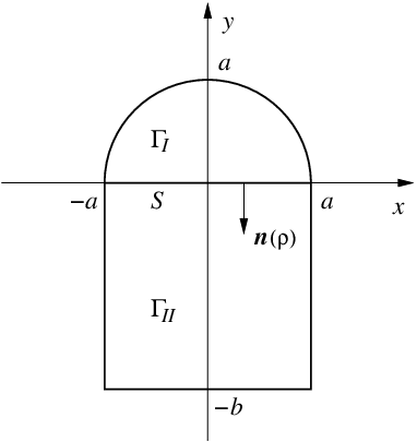
To test the two methods, a few series of numerical calculations have been performed. A system in which Γ\Gamma is a two-dimensional domain consisting of a semicircle of radius aa joined to a rectangle of sides aa and bb, as depicted in figure 2, has been examined.

Refer to caption
Figure 2: Geometry of the system used in the numerical illustration.

The first step is to decide which part of the whole domain Γ\Gamma should be ΓI\Gamma_{I} and which one should be ΓI​I\Gamma_{II}. The decision depends on the simplicity of the construction of the DtN and the NtD operators. The region in which it is easier to solve (40)–(42) should be taken as ΓI​I\Gamma_{II}. In our example the subdomain ΓI\Gamma_{I} is the semicircle and the subdomain ΓI​I\Gamma_{II} is the rectangle. It is not difficult to verify that the eigenvalues of (40)–(42) in this case are

bn​(κ)={−κ2−n2​π2/4​a2​cot⁡(κ2−n2​π2/4​a2​b)forκ2≥n2​π2/4​a2−n2​π2/4​a2−κ2​coth⁡(n2​π2/4​a2−κ2​b)fork2<n2​π2/4​a2,b_{n}(\kappa)=\left\{\begin{array}[]{ccc}-\sqrt{\kappa^{2}-n^{2}\pi^{2}/4a^{2}}\,\cot(\sqrt{\kappa^{2}-n^{2}\pi^{2}/4a^{2}}\,b)&\textrm{for}&\kappa^{2}\geq n^{2}\pi^{2}/4a^{2}\\ -\sqrt{n^{2}\pi^{2}/4a^{2}-\kappa^{2}}\,\coth(\sqrt{n^{2}\pi^{2}/4a^{2}-\kappa^{2}}\,b)&\textrm{for}&k^{2}<n^{2}\pi^{2}/4a^{2}\end{array}\right., (82)

where n=1,2,…n=1,2,\ldots. The corresponding eigenfunctions are of the form

ψn​(κ,x,y)=\displaystyle\psi_{n}(\kappa,x,y)=
An​sin⁡[n​π​(x+a)2​a]​{sin⁡[κ2−n2​π2/4​a2​(y+b)]forκ2≥n2​π2/4​a2sinh⁡[n2​π2/4​a2−κ2​(y+b)]forκ2<n2​π2/4​a2,\displaystyle\quad A_{n}\sin\left[\frac{n\pi(x+a)}{2a}\right]\left\{\begin{array}[]{ccc}\sin\left[\sqrt{\kappa^{2}-n^{2}\pi^{2}/4a^{2}}\,(y+b)\right]&\textrm{for}&\kappa^{2}\geq n^{2}\pi^{2}/4a^{2}\\ \sinh\left[\sqrt{n^{2}\pi^{2}/4a^{2}-\kappa^{2}}\,(y+b)\right]&\textrm{for}&\kappa^{2}<n^{2}\pi^{2}/4a^{2}\end{array}\right.,

where AnA_{n} according to the relation (47) are

An={(a​sin⁡[κ2−n2​π2/4​a2​b])−1forκ2≥n2​π2/4​a2(a​sinh⁡[n2​π2/4​a2−κ2​b])−1forκ2<n2​π2/4​a2.A_{n}=\left\{\begin{array}[]{ccc}\left(\sqrt{a}\,\sin\left[\sqrt{\kappa^{2}-n^{2}\pi^{2}/4a^{2}}\,b\right]\right)^{-1}&\textrm{for}&\kappa^{2}\geq n^{2}\pi^{2}/4a^{2}\\ \left(\sqrt{a}\,\sinh\left[\sqrt{n^{2}\pi^{2}/4a^{2}-\kappa^{2}}\,b\right]\right)^{-1}&\textrm{for}&\kappa^{2}<n^{2}\pi^{2}/4a^{2}\end{array}\right.. (86)

Using equations (82)–(86) in (51) and (52), we obtain the kernels of the DtN and NtD operators. Let us observe that in the examined case we may distinguish the even (symmetric with respect to the y-axis) and the odd (antisymmetric) modes. We may search for them separately (which means working with smaller matrices), applying apropriate basis functions {ϕμ​(𝐫)}\{\phi_{\mu}(\mathbf{r})\} in (61). For the even modes we may use

ϕ1​(𝐫)=r−a,𝐫∈ΓI,\displaystyle\phi_{1}(\mathbf{r})=r-a,\quad\mathbf{r}\in\Gamma_{I}, (87)
ϕμ​(𝐫)=ϕn​m​(𝐫)=r​sin⁡[n​α​(r−a)]​cos⁡(m​β​φ),𝐫∈ΓI\displaystyle\phi_{\mu}(\mathbf{r})=\phi_{nm}(\mathbf{r})=r\sin[n\alpha(r-a)]\cos(m\beta\varphi),\quad\mathbf{r}\in\Gamma_{I} (88)
(μ=2,3,…,n,m=1,2,…)\displaystyle\qquad\qquad\qquad(\mu=2,3,\ldots,\quad n,m=1,2,\ldots)

and for the odd modes we may apply

ϕμ​(𝐫)=ϕn​m​(𝐫)=r​sin⁡[n​α​(r−a)]​sin⁡(m​β​φ),𝐫∈ΓI\displaystyle\phi_{\mu}(\mathbf{r})=\phi_{nm}(\mathbf{r})=r\sin[n\alpha(r-a)]\sin(m\beta\varphi),\quad\mathbf{r}\in\Gamma_{I} (89)
(μ=1,2,…,n,m=1,2,…)\displaystyle\qquad\qquad\qquad(\mu=1,2,\ldots,\quad n,m=1,2,\ldots)

(each μ\mu represents an unique combination of two integers nn and mm). In the above formulas φ\varphi is the angle between the y-axis and the position vector 𝐫=[x,y]\mathbf{r}=[x,y] (we assume that φ\varphi is positive for x<0x<0 and negative for x>0x>0), rr is the length of 𝐫\mathbf{r}, while α\alpha and β\beta are some arbitrary real parameters. Note that all the functions vanish on ∂ΓI\partial\Gamma_{I}. The variational bases are formed from the functions with 1≤n≤nm​a​x1\leq n\leq n_{max} and 1≤m≤mm​a​x1\leq m\leq m_{max}. Do not forget about the extra function (87) used for the symmetric states. The function is added to the basis because all the functions (88) are equal to zero at r=0r=0, while in general the eigenfunctions of the even modes may be nonzero at r=0r=0.

To obtain the estimates of some k2k^{2} and Ψ⁡(𝐫)\Psi(\mathbf{r}), we must establish an initial value of κ\kappa (which is some estimate of kk). Then we apply some chosen variational basis, calculate the matrix elements of Λ(D)​(κ)\mathsf{\Lambda}^{(D)}(\kappa) and Δ(D)​(κ)\mathsf{\Delta}^{(D)}(\kappa) or Λ(N)​(κ)\mathsf{\Lambda}^{(N)}(\kappa) and Δ(N)​(κ)\mathsf{\Delta}^{(N)}(\kappa) and solve the matrix system (66) or (76). The resulting eigenvalues {F~γ(D​o​r​N)​(κ)}\{\widetilde{F}_{\gamma}\,^{(D\;or\;N)}(\kappa)\} are used to set new values of κ\kappa (separately for each γ\gamma). We focus ourselves on an arbitrary chosen state, let it be the state with γ=γ′\gamma=\gamma^{\prime}, so we take

κ=F~γ′(D​o​r​N)​(κ).\kappa=\sqrt{\widetilde{F}_{\gamma^{\prime}}\,^{(D\;or\;N)}(\kappa)}. (90)

We find new matrices, solve the new matrix system and obtain new estimates of eigenvalues {F~γ(D​o​r​N)​(κ)}\{\widetilde{F}_{\gamma}\,^{(D\;or\;N)}(\kappa)\} with F~γ′(D​o​r​N)​(κ)\widetilde{F}_{\gamma^{\prime}}\,^{(D\;or\;N)}(\kappa) among them. We then apply (90) again and the iterative procedure repeats until convergence of F~γ′(D​o​r​N)​(κ)\widetilde{F}_{\gamma^{\prime}}\,^{(D\;or\;N)}(\kappa) is achieved.

Iteration ke​v​e​n,1(D)k_{even,1}^{(D)} ke​v​e​n,1(N)k_{even,1}^{(N)} ko​d​d,1(D)k_{odd,1}^{(D)} ko​d​d,1(N)k_{odd,1}^{(N)}
1 2.0633 2.0487 3.4586 3.4200
2 2.0611 2.0604 3.4508 3.4447
3 2.0611 2.0611 3.4507 3.4505
4 2.0611 3.4507 3.4507
5 3.4507
Table 1: Convergence rate of the DtN and the NtD variational estimates of kk of the lowest even mode and the lowest odd mode of the system used in the numerical example. The results obtained by employing the basis functions (87)–(89) with 1≤n≤151\leq n\leq 15 and 1≤m≤151\leq m\leq 15. The inputs for the iteration procedure have been κ=2.0116\kappa=2.0116 for the first even mode and κ=3.3836\kappa=3.3836 for the first odd mode. SI units are used.
nm​a​xn_{max},mm​a​xm_{max} ke​v​e​n,1(D)k_{even,1}^{(D)} ke​v​e​n,2(D)k_{even,2}^{(D)} ko​d​d,1(D)k_{odd,1}^{(D)} ko​d​d,2(D)k_{odd,2}^{(D)}
ke​v​e​n,1(N)k_{even,1}^{(N)} ke​v​e​n,2(N)k_{even,2}^{(N)} ko​d​d,1(N)k_{odd,1}^{(N)} ko​d​d,2(N)k_{odd,2}^{(N)}
3,3 2.0630 3.0745 3.4527 4.2234
2.0628 3.0809 3.4527 4.2234
5,5 2.0611 3.0734 3.4511 4.2200
2.0611 3.0734 3.4511 4.2200
15,15 2.0611 3.0731 3.4507 4.2190
2.0611 3.0731 3.4507 4.2190
25,25 2.0611 3.0730 3.4506 4.2189
2.0611 3.0730 3.4506 4.2189
30,30 2.0611 3.0730 3.4506 4.2189
2.0611 3.0730 3.4506 4.2189
Table 2: Converged DtN and NtD variational estimates of kk of the two lowest even modes and the two lowest odd modes. The basis functions (87)–(89) with 1≤n≤nm​a​x1\leq n\leq n_{max} and 1≤m≤mm​a​x1\leq m\leq m_{max} have been used. The inputs for the iterative procedures have been κ=2.0116\kappa=2.0116 and κ=2.9638\kappa=2.9638 for the even modes and κ=3.3836\kappa=3.3836 and κ=4.0232\kappa=4.0232 for the odd modes. SI units are used.

The numerical calculations have been made for a=1a=1, b=1.5b=1.5 and α=β=1\alpha=\beta=1 (SI units are used). Table 1 presents estimates of kk of the first even mode and the first odd mode obtained by using the iterative procedure described above. The variational bases have contained the functions (87) and (88) (for the even mode) or (89) (for the odd mode) with 1≤n≤151\leq n\leq 15 and 1≤m≤151\leq m\leq 15. The initial values of κ\kappa have been κ=2.0116\kappa=2.0116 for the first even mode and κ=3.3836\kappa=3.3836 for the first odd mode, they are the exact values of kk (with accuracy of 4 decimal places) of the first even mode and the first odd mode of the system (1)–(2) with Γ\Gamma being a rectangle of sides 2 and 2.5 (in the next series of calculations the fact that in case of the rectangle the second even mode is characterized by k=2.9638k=2.9638 and the second odd mode by k=4.0232k=4.0232 has been used). We see that the estimates converge after a few iterations, and that the results obtained by the DtN method converge faster. To verify, how the converged (after the iterative procedure) estimates of kk depend on the basis dimensions, let us analyze the results collected in table 2. The two lowest even modes and the two lowest odd modes of our problem have been examined. The inputs for the iterative procedures have been κ=2.0116\kappa=2.0116 and κ=2.9638\kappa=2.9638 for the even modes and κ=3.3836\kappa=3.3836 and κ=4.0232\kappa=4.0232 for the odd modes. It is seen that even quite small bases lead to estimates of good accuracy. The aim of the next series of numerical calculations was to estimate eigenfunctions Ψ\Psi of the four states. Figure 3 shows density plots of |Ψ|2|\Psi|^{2} of the four modes obtained by using the DtN method in a way presented at the end of section IV. In the domain ΓI\Gamma_{I} the basis functions (87)–(89) with 1≤n≤251\leq n\leq 25 and 1≤m≤251\leq m\leq 25 have been used. The values of κ\kappa have been equal to the converged estimates of kk (see table 2). Density plots obtained by the NtD method are exactly the same.

Refer to caption Refer to caption
Figure 3: Density plots of |Ψ|2|\Psi|^{2}: (a) and (b) – the two lowest even modes; (c) and (d) – the two lowest odd modes. The results obtained by the DtN method (see section IV). The basis functions (87)–(89) with 1≤n≤251\leq n\leq 25 and 1≤m≤251\leq m\leq 25 have been used. The converged estimates of kk (see the last row of table 2) have been taken as the values of κ\kappa.

Acknowledgments
I wish to thank Professor R. Szmytkowski for many useful discussions.

References

  • [1] P. Amore, J. Phys. A: Math. Theor. 41, 265206/1–29 (2008)
  • [2] S. Chakraborty, J. K. Bhattacharjee, S. P. Khastgir, J. Phys. A: Math. Theor. 42, 195301/1–12 (2009)
  • [3] O. Steinbach, M. Windisch, Numer. Math. DOI: 10.1007/s00211-010-0315-6 (2010)
  • [4] R. Szmytkowski, S. Bielski, Phys. Rev. A 70, 042103/1–12 (2004)
  • [5] S. Bielski, R. Szmytkowski, J. Phys. A 39, 7359–7381 (2006)
  • [6] J. E. Inglesfield, J. Phys. C 14, 3795–3806 (1981)
  • [7] R. Szmytkowski, J. Phys. A: Math. Gen. 30, 4413–4438 (1997)
  • [8] R. Szmytkowski, J. Math. Phys. 39, (1998) 5231–5252, Erratum: J. Math. Phys. 40, 4181 (1999)
  • [9] E. Gerjuoy, A. R. P. Rau, L. Spruch, Rev. Mod. Phys. 55, 725–774 (1983)
  • [10] R. Szmytkowski, S. Bielski, Int. J. Quantum Chem. 97, 966–976 (2004)
  • [11] G. Auchmuty, Num. Funct. Anal. Opt. 25, 321–348 (2004)