Uncertainty Updating in the Description of Coupled Heat and Moisture Transport in Heterogeneous Materials

There are many important factors limiting the service life of buildings. An appropriate reliability analysis needs to take into account uncertainties in the environmental conditions as well as in structural properties. Thanks to the growth of powerful computing resources and technology, recently developed procedures in the field of stochastic mechanics have become applicable to realistic engineering systems.

The most common methods quantifying uncertainties are the first- and second-order reliability methods (FORM/SORM [3]) computing the probability of failure related to limit states. Nevertheless, modern sophisticated and highly nonlinear models lead to non-Gaussian higher-order probability density functions of model parameters and its response. The higher moments become interesting quantities to be estimated by probabilistic analysis such as stochastic finite element methods (SFEM), see e.g. [4] for a recent review. SFEM is a powerful tool in computational stochastic mechanics extending the classical deterministic finite element method (FEM) to the stochastic framework involving finite elements whose properties are random.

This paper is focused on the modelling of uncertainties in material properties and investigates the influence of such uncertainties on structural response. When dealing with homogeneous materials, one obtains a simplified scenario for SFEM, where uncertain material properties are described by random variables, which are assumed to be spatially constant. In the field of heterogeneous materials modelling, a widespread approach is multiscale modelling based on homogenization as presented e.g. in [5, 6, 7]. Nevertheless, homogenization theories have rigorous foundations for materials with well-defined geometry and components described by simple constitutive laws as in the case of regular masonry or composite materials with periodic microstructure. However, these techniques cannot be efficiently applied to materials with random microstructure such as in case of quarry masonry, see Fig. 1.

Another possibility is casting the description of heterogenous material within the probabilistic framework, where uncertain material properties in time and/or space are represented by stochastic processes and fields. The resulting problem can be then solved by different strategies. The most famous group involves spectral stochastic finite element methods (SSFEM) [8]. These methods of uncertainty quantification are focused on propagation of uncertainty in the system properties through the numerical model of the system in order to estimate probabilistic quantification of structural response. It assumes the knowledge of probabilistic formulation of uncertain system properties. Nevertheless, this uncertainty is usually very high before the structure is built, but after the construction, practical measurements can be performed. With these observations, the probabilistic models can be updated, to give a more accurate and reliable estimate. To this goal, the appropriate techniques from the field of inverse analysis should be employed.

The following section presents a brief introduction into the inverse analysis. Section 3 is devoted to Bayesian inference suitable for probabilistic estimation of model parameters from noisy and limited data. Section 4 is focused on the probabilistic description of heterogeneous materials properties where particular material parameters are not spatially constant. Section 5 presents the application of Bayesian inference to model of coupled heat and moisture transfer in heterogeneous material and the obtained results are concluded in Section 6.

In computational mechanics one tries to model a real system $\mathsf{A}$, where system parameters $\mathsf{q}$, a loading $\mathsf{f}$ and a system response $\mathsf{u}$ are related as

The goal here is to obtain the response of the system for given parameters and loading conditions. In the field of inverse analysis, the goal is to find the values of system parameters $\mathsf{q}$ corresponding to given loading conditions $\mathsf{f}$ and experimental observations $\mathsf{z}$. Therefore, one uses the numerical model of the system $\mathsf{A}$ and derives a so-called observation operator $\mathsf{Y}$ mapping the response $\mathsf{u}$ given parameters $\mathsf{q}$ and loading $\mathsf{f}$ to observed quantities $\mathsf{z}$

The subject of this work is concerned with the description of heat and moisture conduction in structural materials and the system parameters $\mathsf{q}$ are related here to the material behaviour. Material parameters are usually determined in the context of a chosen experimental setup, where the loading conditions are fixed, hence, the loading $\mathsf{f}$ is assumed to be constant in the following text.

When simulating some real experiment, the model response is usually not equal to measured data because of experimental errors or imperfection of numerical model itself. It is often difficult to distinguish these sources of errors and they are described together in error vector $\mathsf{\epsilon}$, so Eq. (2) becomes

The most common way of estimating material properties is based on fitting the response of numerical model to the results of real experiments, see e.g. [9] for a recent review of parameters identification strategies. This usually leads to an optimization problem, where the difference between the model response and measured data is minimized by an appropriate optimization algorithm. Nevertheless, the formulation of the suitable error function is not always trivial [10, 11, 12]. The resulting function is often multimodal, non-smooth or non-differentiable and some robust optimization algorithm must be used (see e.g. [13] for an illustrative example of an application of evolutionary algorithm to solve such problem).

There are only several works on including uncertainties into the curve fitting-based approach to parameters identification as e.g. in [14]. In general, these approaches omit related uncertainties in measurements as well as imperfections of the numerical model and also the preliminary knowledge about the material parameters coming from their physical meaning (e.g. Young’s modulus must be positive, Poisson’s ratio must lay within the $-1$ and $0.5$, etc).

Bayesian inference is the statistical inference in which the experimental observations are not used as the only source of information, but they are used to update the preliminary probabilistic description of system - the so-called prior information - to give the posterior distribution [15]. Recall that in realistic applications, observations are noisy, uncertain and limited in number relative to the dimension or complexity of the model space. Also, the model of a system may have limitations on its predictive value because of its imprecision, filtering or smoothing effects. Taking into account all pertinent uncertainties, the process of material properties estimation cannot lead to a single ’optimal’ parameter set, but one has to find a probability distribution of parameters that represents the knowledge about parameter values. The Bayesian setting for the inverse problems offers a rigorous foundation for inference from noisy data and uncertain forward models, a natural mechanism for incorporating prior information, and a quantitative assessment of uncertainty in the inferred results summarizing all available information about the unknown quantity [1]. In addition, unlike other techniques that aim to regularize the ill-posed inverse problem to achieve a point estimate, the Bayesian method treats the inverse problem as a well-posed problem in an expanded stochastic space.

The Bayesian approaches to inverse problems have received much recent interest, since increasing performance of modern computers and clusters enables exhaustive Monte Carlo computations. Among recent applications one can cite applications in environmental modelling [16], hydrology [17] or heat transfer [18]. We review this approach briefly below; for more extensive introductions, see [1].

The main principle of Bayesian inference is casting the inverse problem in the probabilistic setting, where material parameters $\mathsf{q}$ as well as observations $\mathsf{z}$ and also the response of forward operator $\mathsf{Y}(\cdot)$ are considered as random variables or random fields. Therefore, we introduce the following notation. We consider a set $\mathit{\Omega}$ of random elementary events $\omega$ together with $\sigma$-algebra $\mathscr{S}$ to which a real number in the interval $[0,1]$ may be assigned, the probability of occurrence - mathematically a measure $\mathbb{P}$.

In the Bayesian setting, we assume three sources of information and uncertainties, which should be taken into account. The first one is our prior knowledge about the model/material parameters $\mathsf{q}(\omega)$, which is represented by defining the prior density function $p_{\mathsf{q}}(\mathsf{q})$. Prior models may embody simple constraints on $\mathsf{q}$, such as a range of feasible values, or may reflect more detailed knowledge about the parameters, such as correlations or smoothness.

Other source of information comes from measurements, which are violated by uncertain experimental errors $\mathsf{\epsilon}(\bar{\omega})$. Last uncertainty arises from imperfection of the numerical model included in the observation operator $\mathsf{Y}(\cdot)$, when for example our description of the real system $\mathsf{A}$ does not include all important phenomena and therefore the forward operator response $\mathsf{Y}(\cdot,\bar{\bar{\omega}})$ can be assumed as uncertain. The probabilistic formulation of Eq. (3) now becomes

If modelling uncertainties $\bar{\bar{\omega}}$ cannot be neglected, they can be described by conditional probability density $p(\mathsf{z}|\mathsf{q})$ for predicted data $\mathsf{z}$ and given model parameters $\mathsf{q}$. If these uncertainties can be neglected, only model parameters $\mathsf{q}(\omega)$ and observations $\mathsf{z}(\bar{\omega})$ remain uncertain. In practise, it is sometimes difficult to distinguish the imperfection of the system description $\mathsf{A}$ from measurement error $\mathsf{\epsilon}$. Hence modelling uncertainties $\bar{\bar{\omega}}$ can be hidden in measuring error $\mathsf{\epsilon}(\bar{\omega})$. Finally, for noisy measurements we define the last probability density $p_{\mathsf{z}}(\mathsf{z})$.

To update our prior knowledge about model parameters we must include measurements with our theoretical knowledge. Bayesian update is based on the idea of Bayes’ rule defined for probabilities. Definition of Bayes’ rule for continuous distribution is, however, more problematic and hence [1, Chapter 1.5] derived the posterior state of information $\pi(\mathsf{q},\mathsf{z})$ as a conjunction of all information at hand

where $\kappa$ is a normalization constant.

The posterior state of information defined in the space of model parameters $\mathsf{q}$ is given by the marginal probability density

where $\mathit{\bar{\Omega}}$ is a set of random elementary events $\bar{\omega}$ and measured data $\mathsf{z}$ enters through the likelihood function $L(\mathsf{q})$, which gives a measure of how good a forward operator $\mathsf{Y}(\mathsf{q})$ is in explaining the data $\mathsf{z}$. Here, $\mathbb{E}_{\bar{\omega}}$ is the expectation operator averaging over $\mathit{\bar{\Omega}}$.

To keep the presentation of different numerical aspects of particular methods clear and transparent, we focus here on a quite common and simple case, where modelling-uncertainties are neglected and measurement errors are assumed to be Gaussian. Then the likelihood function takes the form

where $C_{\mathrm{obs}}$ is a covariance among measurements $\mathsf{z}$.

The primary computational challenge is extracting information from the posterior density $\pi_{\mathsf{q}}(\mathsf{q})$ [1]. Most estimates take the form of integrals over the posterior, which may be computed with asymptotic methods, deterministic methods, or sampling. The deterministic quadrature or cubature may be attractive alternatives to Monte Carlo simulation at low to moderate dimensions, but Markov chain Monte Carlo (MCMC) [19] remains the most general and flexible method for complex and high-dimensional distributions.

In modelling of heterogeneous material, some material parameters are not constants, but can be described as random fields. It means that the uncertainty in the particular material parameter $q$ is modelled by defining $q(\mathchoice{\displaystyle\boldsymbol{x}}{\textstyle\boldsymbol{x}}{\scriptstyle\boldsymbol{x}}{\scriptscriptstyle\boldsymbol{x}})$ for each $\mathchoice{\displaystyle\boldsymbol{x}}{\textstyle\boldsymbol{x}}{\scriptstyle\boldsymbol{x}}{\scriptscriptstyle\boldsymbol{x}}\in\mathcal{G}$ as a random variable $q(\mathchoice{\displaystyle\boldsymbol{x}}{\textstyle\boldsymbol{x}}{\scriptstyle\boldsymbol{x}}{\scriptscriptstyle\boldsymbol{x}}):\mathit{\Omega}\rightarrow\mathbb{R}$ on a suitable probability space $(\mathit{\Omega},\mathscr{S},\mathbb{P})$ in some bounded admissible region $\mathcal{G}\subset\mathbb{R}^{d}$. As a consequence, $q:\mathcal{G}\times\mathit{\Omega}\rightarrow\mathbb{R}$ is a random field and one may identify $\mathit{\Omega}$ with the set of all possible values of $q$ or with the space of all real-valued functions on $\mathcal{G}$. Alternatively, $q(\mathchoice{\displaystyle\boldsymbol{x}}{\textstyle\boldsymbol{x}}{\scriptstyle\boldsymbol{x}}{\scriptscriptstyle\boldsymbol{x}},\omega)$ can be seen as a collection of real-valued random variables indexed by $\mathchoice{\displaystyle\boldsymbol{x}}{\textstyle\boldsymbol{x}}{\scriptstyle\boldsymbol{x}}{\scriptscriptstyle\boldsymbol{x}}\in\mathcal{G}$.

Assuming the random field $q(\mathchoice{\displaystyle\boldsymbol{x}}{\textstyle\boldsymbol{x}}{\scriptstyle\boldsymbol{x}}{\scriptscriptstyle\boldsymbol{x}},\omega)$ to be Gaussian, it is defined by its mean

and its covariance

Some non-Gaussian fields may be synthesized as – usually nonlinear – functions of Gaussian fields [20, 21]. For instance, most of the material parameters cannot be negative, hence, the lognormal random field can be more suitable for their description. Then the lognormal random field $q(\mathchoice{\displaystyle\boldsymbol{x}}{\textstyle\boldsymbol{x}}{\scriptstyle\boldsymbol{x}}{\scriptscriptstyle\boldsymbol{x}},\omega)$ for each material parameter is obtained by nonlinear transformation of a standard Gaussian random field $q_{g}(\mathchoice{\displaystyle\boldsymbol{x}}{\textstyle\boldsymbol{x}}{\scriptstyle\boldsymbol{x}}{\scriptscriptstyle\boldsymbol{x}},\omega)$ as, given in [21],

The statistical moments $\mu_{g}$ and $\sigma_{g}$ can be obtained from statistical moments $\mu_{q}$ and $\sigma_{q}$ given for lognormally distributed material property according to following relations:

In a computational setting, the random field and the numerical model must be discretized. If the parameter field $q(\mathchoice{\displaystyle\boldsymbol{x}}{\textstyle\boldsymbol{x}}{\scriptstyle\boldsymbol{x}}{\scriptscriptstyle\boldsymbol{x}})$ can be adequately represented on a finite collection of points $\{{\mathchoice{\displaystyle\boldsymbol{x}}{\textstyle\boldsymbol{x}}{\scriptstyle\boldsymbol{x}}{\scriptscriptstyle\boldsymbol{x}}}^{n}_{i=1}\}\in\mathbb{R}^{2}$, then we can write both the prior and posterior densities in terms of $\mathchoice{\displaystyle\boldsymbol{q}}{\textstyle\boldsymbol{q}}{\scriptstyle\boldsymbol{q}}{\scriptscriptstyle\boldsymbol{q}}=(q(\mathchoice{\displaystyle\boldsymbol{x}}{\textstyle\boldsymbol{x}}{\scriptstyle\boldsymbol{x}}{\scriptscriptstyle\boldsymbol{x}}_{1}),\dots,q(\mathchoice{\displaystyle\boldsymbol{x}}{\textstyle\boldsymbol{x}}{\scriptstyle\boldsymbol{x}}{\scriptscriptstyle\boldsymbol{x}}_{n}))$, where $q_{i}=q(\mathchoice{\displaystyle\boldsymbol{x}}{\textstyle\boldsymbol{x}}{\scriptstyle\boldsymbol{x}}{\scriptscriptstyle\boldsymbol{x}}_{i})$ are random variables usually correlated among each other. The vector $\mathchoice{\displaystyle\boldsymbol{q}}{\textstyle\boldsymbol{q}}{\scriptstyle\boldsymbol{q}}{\scriptscriptstyle\boldsymbol{q}}$, however, will probably be high-dimensional and it renders MCMC exploration of the posterior more challenging. Therefore, the Karhunen$-$Loève expansion (KLE) can be applied to dimensionality reduction [22].

KLE is an extremely useful tool for the concise representation of the stochastic processes. Based on the spectral decomposition of covariance function $C_{q}(\mathchoice{\displaystyle\boldsymbol{x}}{\textstyle\boldsymbol{x}}{\scriptstyle\boldsymbol{x}}{\scriptscriptstyle\boldsymbol{x}},\mathchoice{\displaystyle\boldsymbol{x}}{\textstyle\boldsymbol{x}}{\scriptstyle\boldsymbol{x}}{\scriptscriptstyle\boldsymbol{x}}^{\prime})$ and the orthogonality of eigenfunctions $\psi_{i}$, the random field $q(\mathchoice{\displaystyle\boldsymbol{x}}{\textstyle\boldsymbol{x}}{\scriptstyle\boldsymbol{x}}{\scriptscriptstyle\boldsymbol{x}},\omega)$ can be written as

where $\mathchoice{\displaystyle\boldsymbol{\xi}}{\textstyle\boldsymbol{\xi}}{\scriptstyle\boldsymbol{\xi}}{\scriptscriptstyle\boldsymbol{\xi}}(\omega)=(\ldots,\xi_{i}(\omega),\ldots)^{\mathrm{T}}$ is a set of uncorrelated random variables of zero mean and unit variance. The spatial KLE functions $\psi_{i}(\mathchoice{\displaystyle\boldsymbol{x}}{\textstyle\boldsymbol{x}}{\scriptstyle\boldsymbol{x}}{\scriptscriptstyle\boldsymbol{x}})$ are the eigenfunctions of the Fredholm integral equation with the covariance function as the integral kernel:

where $\varsigma_{i}$ are positive eigenvalues ordered in a descending order.

Since the covariance is symmetric and positive definite, it can be expanded in the series

However, computing the eigenfunctions analytically is usually not feasible. Therefore, one discretizes the covariance spatially according to chosen grid points (usually corresponding to a finite element mesh). The resulting covariance matrix $\mathchoice{\displaystyle\mathbf{C}}{\textstyle\mathbf{C}}{\scriptstyle\mathbf{C}}{\scriptscriptstyle\mathbf{C}}_{q}$ is again symmetric and positive definite and Eq. (13) becomes symmetric matrix eigenvalue problem, see [23], where the eigenfunctions $\psi_{i}(\mathchoice{\displaystyle\boldsymbol{x}}{\textstyle\boldsymbol{x}}{\scriptstyle\boldsymbol{x}}{\scriptscriptstyle\boldsymbol{x}})$ are replaced by eigenvectors $\mathchoice{\displaystyle\boldsymbol{\psi}}{\textstyle\boldsymbol{\psi}}{\scriptstyle\boldsymbol{\psi}}{\scriptscriptstyle\boldsymbol{\psi}}_{i}$. The eigenvalue problem is usually solved by a Krylov subspace method with a sparse matrix approximation. For large eigenvalue problems, [24] proposes the efficient low-rank and data sparse hierarchical matrix techniques.

For practical implementation, the series (12) and (14) are truncated after $M$ terms, yielding the approximations

Such spatial semi-discretization is optimal in the sense that the mean square error resulting from a truncation after the $M$-th term is minimized.

This section is devoted to application of previously described techniques to uncertainty updating in coupled heat and moisture transport in heterogeneous material with uncertain structure as quarry masonry. In particular, we employ the model proposed by Künzel [2] described by the energy balance equation

and the conservation of mass equation

where $\theta$ is the temperature, $\varphi$ stands for the moisture and $H$, $\lambda$, etc are described below. The transport coefficients defining the material behaviour are nonlinear functions of structural responses - the temperature and moisture fields - and material properties. We briefly recall their particular relations [2]:

• 1.

  Thermal conductivity $[\mathrm{Wm}^{-1}\mathrm{K}^{-1}]$:

  $$\lambda=\lambda_{0}\left(1+\frac{b_{\mathrm{tcs}}w_{f}(b-1)\varphi}{\rho_{s}(b-\varphi)}\right)\,.$$

  (19)

• 2.

  Evaporation enthalpy of water $[\mathrm{Jkg}^{-1}]$:

  $$h_{v}=2.5008\cdot 10^{6}\left(\frac{273.15}{\theta}\right)^{(0.167+3.67\cdot 10^{-4}\theta)}\,.$$

  (20)

• 3.

  Water vapour permeability $[\mathrm{kgm}^{-1}\mathrm{s}^{-1}\mathrm{Pa}^{-1}]$:

  $$\delta_{p}=\frac{1.9446\cdot 10^{-12}}{\mu}\cdot\left(\theta+273.15\right)^{0.81}\,.$$

  (21)

• 4.

  Water vapour saturation pressure $[\mathrm{Pa}]$:

  $$p_{\mathrm{sat}}=611\exp\left(\frac{17.08\theta}{234.18+\theta}\right)\,.$$

  (22)

• 5.

  Liquid conduction coefficient $[\mathrm{kgm}^{-1}\mathrm{s}^{-1}]$:

  $$D_{\varphi}=3.8\frac{a^{2}}{w_{f}}\cdot 10^{\frac{3w_{f}(b-1)\varphi}{(b-\varphi)(w_{f}-1)}}\cdot\frac{b(b-1)}{(b-\varphi)^{2}}\,.$$

  (23)

• 6.

  Total enthalpy of building material $[\mathrm{Jm}^{-3}]$:

  $$H=\rho_{s}c_{s}\theta\,.$$

  (24)

More detailed discussion about transport coefficients can be found in [2, 25]. Some transport coefficients defined by Eqs. (19) - (24) depend on a subset of the material parameters listed in Tab. 1. The approximation factor $b$ appearing in Eqs. (19) and (23) can be determined from the relation:

where $w_{80}$ is the equilibrium water content at $0.8\,\mathrm{[-]}$ relative humidity. Therefore, $b$ is not considered as a material parameter, while $w_{80}$ is another material property to be determined. Finally, there are $8$ material parameters listed in Tab. 1 to be estimated by updating procedure.

The presented table also contains the prior information about material parameters in terms of the mean values $\mu_{q}$ and the standard deviations $\sigma_{q}$. Their particular values are chosen with regard to values corresponding to materials used in masonry [26]. Other prior information is that all these material parameters cannot be negative and hence, they could be considered as lognormally distributed. To describe the uncertainty about parameters of heterogeneous material, we choose the covariance kernel of a corresponding random field. Since the material properties change in the space because of changes in material components, we assume that the spatial fluctuations of all parameters are equal. It is probably not the best description of a real material. Nevertheless, we are convinced that the full spatial correlation among material properties is more realistic then full spatial independence. For the sake of simplicity, we do not study here the case of arbitrarily correlated parameters. Therefore, we assume the same normalized exponential covariance kernel for all parameters,

where $l_{x_{1}}$ and $l_{x_{2}}$ are covariance lengths. We assume also that the expert is certain about correlation lengths $l_{x_{1}}=0.1$ $\mathrm{[m]}$ and $l_{x_{2}}=0.04$ $\mathrm{[m]}$, but he is not sure about a particular distribution of phases in material. In practise, the correlation lengths can be determined by the image analysis of a given material [27], common size of bricks in masonry etc.

Utilizing the covariance kernel (26), we compute particular realizations of standard Gaussian random field based on Karhunen-Loève expansion

Here, the eigenvectors $\mathchoice{\displaystyle\boldsymbol{\psi}}{\textstyle\boldsymbol{\psi}}{\scriptstyle\boldsymbol{\psi}}{\scriptscriptstyle\boldsymbol{\psi}}_{i}$ describe the fluctuation of material property within the studied domain $\mathcal{G}$. Since the fluctuations reflect here the distribution of phases in material, the random variables $\xi_{i}$ are also considered same for all material parameters. Given the prior mean $\mu_{q}$ and standard deviation $\sigma_{q}$ for each material parameter in Tab. 1, corresponding statistical moments $\mu_{g}$ and $\sigma_{g}$ can be derived from Eq. (11). These can be then applied to Eq. (10) in order to obtain a lognormal random field for each material parameter. Nevertheless, such procedure implies that the expert is also certain about mean value and relative amplitudes (given by the prior standard deviation) of respective random fields. That will unlikely happen in practice. To make the example more realistic, we include the uncertainty in the mean values of particular random fields by adding one random variable $\xi_{q,0}$ for each material property and extending the Eq. (10) into

As a result, the random field corresponding to particular material property can be now shifted independently to each other. For a sake of simplicity and to keep the number of random variables in reasonable bounds, we keep the amplitudes of respective random fields still closely related. The total number of random variables $L$ to be updated within Bayesian framework now becomes $L=M+W$, where $M$ is the number of terms in the truncated KL expansion and $W$ is the number of material properties.

As an example, we consider two-dimensional rectangular domain discretized by FE mesh into $80$ nodes and $120$ elements. Its geometry together with the specific loading conditions are shown in Fig. 2. The initial temperature is $\theta_{\mathrm{in}}=14$ [^∘C] and moisture $\varphi_{\mathrm{in}}=0.5$ [-] in the whole domain. One side of the domain is submitted to exterior loading conditions $\theta_{\mathrm{ext}}=5$ [^∘C] and $\varphi_{\mathrm{ext}}=0.5$ [-], while the opposite side is submitted to interior loading conditions $\theta_{\mathrm{int}}=24$ [^∘C] and $\varphi_{\mathrm{int}}=0.8$ [-].

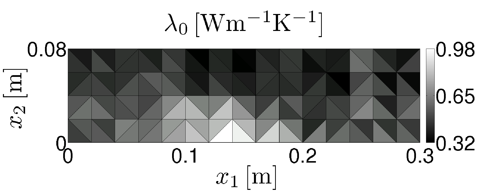
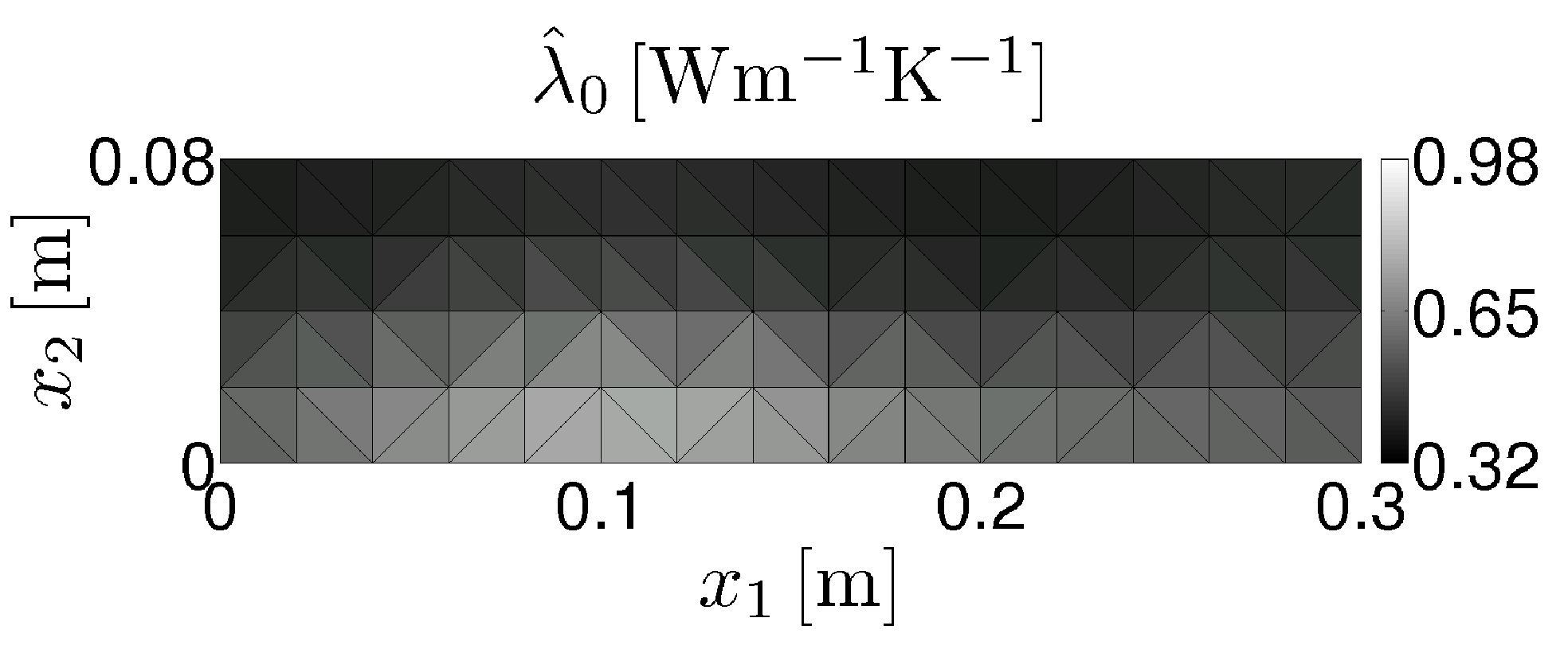
In order to reduce the number of random variables to be updated within the Bayesian inference, one needs to choose the number of eigenmodes $M$ as small as possible, but high enough for a satisfactory description of parameter fields. The attention should be paid to the error in description of parameter fields as well as to the related error in the model response. Fig. 3 presents a comparison of an arbitrary realization of thermal conductivity field $\lambda_{0}(\mathchoice{\displaystyle\boldsymbol{x}}{\textstyle\boldsymbol{x}}{\scriptstyle\boldsymbol{x}}{\scriptscriptstyle\boldsymbol{x}})$ computed using all $120$ eigenmodes and its approximation $\hat{\lambda}_{0}(\mathchoice{\displaystyle\boldsymbol{x}}{\textstyle\boldsymbol{x}}{\scriptstyle\boldsymbol{x}}{\scriptscriptstyle\boldsymbol{x}})$ computed using only first $7$ eigenmodes.

When comparing the corresponding heat and moisture fields, the negligence of higher eigenmodes in description of input parameter fields is reflected by fluctuations of response fields. These are, however, relatively small comparing to absolute values of temperature and moisture (see Fig. 6). For better understanding, Fig. 4 shows only the fluctuations of response fields, since we have subtracted the response fields ($\bar{\theta}(\mathchoice{\displaystyle\boldsymbol{x}}{\textstyle\boldsymbol{x}}{\scriptstyle\boldsymbol{x}}{\scriptscriptstyle\boldsymbol{x}})$ and $\bar{\varphi}(\mathchoice{\displaystyle\boldsymbol{x}}{\textstyle\boldsymbol{x}}{\scriptstyle\boldsymbol{x}}{\scriptscriptstyle\boldsymbol{x}})$) corresponding to homogeneous medium. (The particular response fields correspond to time $t=200$ $\mathrm{[h]}$.)

One can conclude that the employed Künzel’s model has a smoothing effect, because negligence of higher eigenmodes induced relatively high error in the approximation of input parameter fields, while its impact to the fluctuations of response fields is almost vanishing.

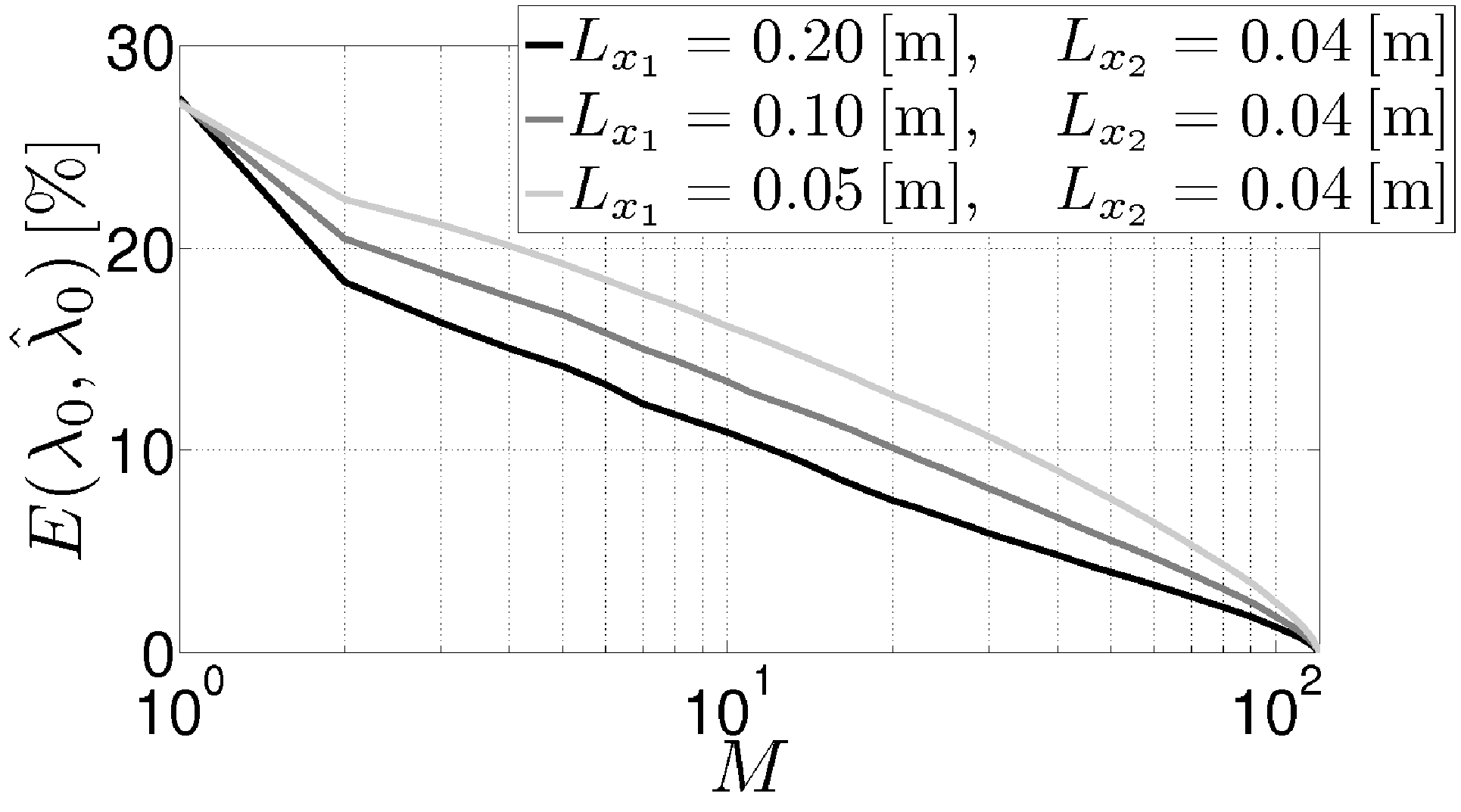
In order to choose an appropriate number of eigenmodes, a relative point-wise error of input fields averaged over all $120$ finite elements and over $100$ independent random realizations can be computed according to

A similar error can be also computed in terms of response fields. These errors as a function of the number of eigenmodes $M$ involved in the description of input fields computed for three different choices of correlation lengths are depicted in Fig. 5. It can be seen again that the error in description of input fields is decreasing slowly, while the error in the response fields descends much faster due to the smoothing effect of the numerical model. Owing to the results in Fig. 5, we decided to perform the Bayesian inference with an approximation of input fields using $7$ KLE modes, which provides a satisfactory accuracy.

According to the formulation of lognormal input fields given in Eq. (28), we use one random variable for each eigenmode involved (it is $M=7$) and one random variable for each material properties (it is $W=8$) in order to enable their relative shift. Hence, we have $L=15$ random variables to be updated within the Bayesian inference.

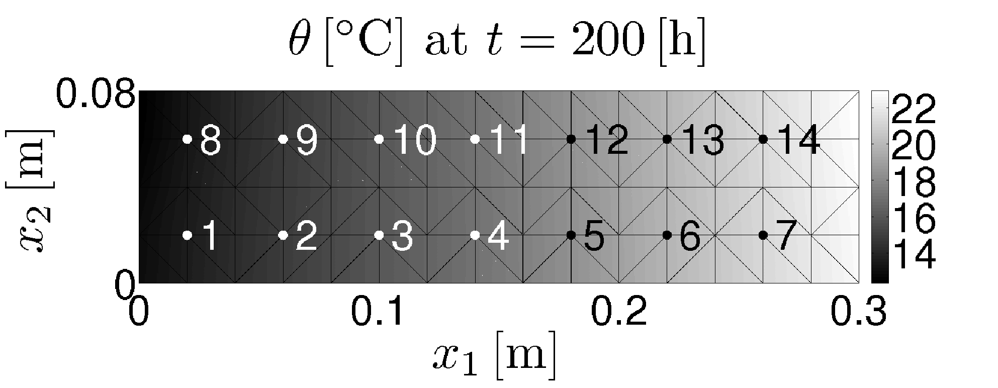
Due to the lack of experimental data, we prepared a virtual experiment based on simulation including all eigenmodes. The values of temperature and moisture are measured in 14 points shown at Figs. 6 (a) and (c) and at three distinct times given in Figs. 6 (b) and (d). Hence, the observations $\mathchoice{\displaystyle\boldsymbol{d}}{\textstyle\boldsymbol{d}}{\scriptstyle\boldsymbol{d}}{\scriptscriptstyle\boldsymbol{d}}$ consist of $84$ values. They were then perturbed by Gaussian noise with standard deviation for temperature $\sigma_{\theta}=0.2$ $\mathrm{[^{\circ}C]}$ and for moisture $\sigma_{\varphi}=0.02$ $\mathrm{[-]}$ and in that way we produced $100$ virtual measurements. Based on them we calculated the observation covariance matrix $\mathchoice{\displaystyle\mathbf{C}}{\textstyle\mathbf{C}}{\scriptstyle\mathbf{C}}{\scriptscriptstyle\mathbf{C}}_{\mathrm{obs}}$ appearing in the likelihood function, which has the Gaussian form shown in the Eq. (7).

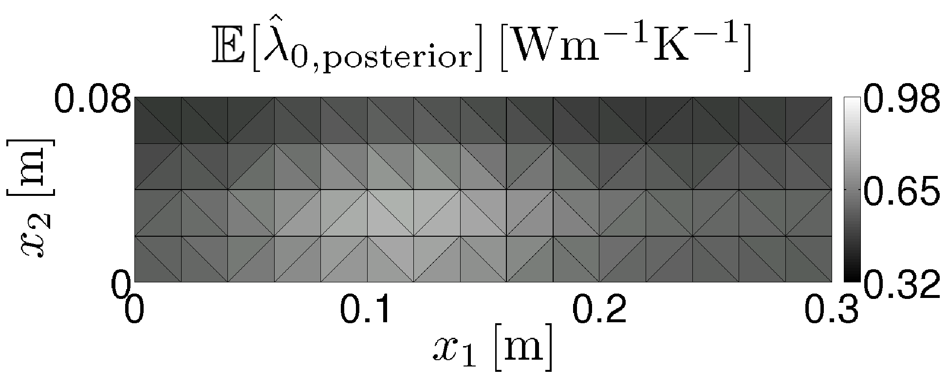
The Bayesian update was performed using Metropolis-Hasting algorithm and $80,000$ samples were generated in order to sample the posterior density (5) over variables $\mathchoice{\displaystyle\boldsymbol{\xi}}{\textstyle\boldsymbol{\xi}}{\scriptstyle\boldsymbol{\xi}}{\scriptscriptstyle\boldsymbol{\xi}}=(\xi_{1}\dots\xi_{15})$. Then, one realization of parameter fields was computed for each sample vector $\mathchoice{\displaystyle\boldsymbol{\xi}}{\textstyle\boldsymbol{\xi}}{\scriptstyle\boldsymbol{\xi}}{\scriptscriptstyle\boldsymbol{\xi}}$. The mean computed over all posterior fields of thermal conductivity $\mathbb{E}[\hat{\lambda}_{0,\mathrm{posterior}}]$ depicted in Fig. 7 (a) can be compared with the reference field in Fig. 3 (a) utilized for preparation of virtual experiment.

Since the mean is not a sufficient descriptor of the a posteriori distribution, Fig. 7 (b) shows a cut of a subset of $200$ posterior samples (light grey lines). The cut is driven along the axis $x$ at $y=0.03$ $\mathrm{[m]}$. These posterior samples can be compared with the same number of fields computed for samples drawn from the a priori distribution (dark grey lines) and the cut through the reference field of $\lambda_{0}$ (bold black line). One can see that the a posteriori samples much better encompass the reference field than the a priori ones.

During the updating process, the model responses obtained for the a posteriori samples were stored. Fig. 8 shows the difference between the reference response fields and the mean computed over posterior response fields, both at time $t=200$ $\mathrm{[h]}$. Comparing the differences in Fig. 8 with size of fluctuations of corresponding fields in Figs. 4 (a) and (b), one can conclude that the differences are relatively small.

Finally, the a posteriori and the a priori distributions of the responses can be compared with the reference response at Fig. 9. The figure shows the evolution of the temperature (a) and the moisture (b) in time at the FE node no. $4$. It is evident from the figures that the a posteriori samples (light grey) are distributed in the very vicinity of the reference response (bold black), while the dispersion of responses computed for $200$ samples drawn from the a priori distribution is very large.

The presented paper deals with the Bayesian updating of uncertainty in properties of heterogeneous materials. The process starts with the a priori highly uncertain information given by an expert about material properties, which enters as input into the chosen material model. The model employed here is the Künzel’s model of coupled heat and moisture transfer, which assumes highly nonlinear relation between $8$ material parameters and the structural response as given in Eqs. (19) – (24). Beside the prior uncertainty in the value of material characteristic itself, another uncertainty arises when describing heterogeneous material with spatial fluctuations of such property. In order to describe the fluctuations, one random field is assigned to each material property. For a sake of simplicity, the fully correlated random fields are assumed, but one random variable is added into the description of each parameter so as to allow their mutual shift. To limit the number of random variables describing the material, the random fields are approximated by Karhunen-Loève expansion with 7 eigenmodes. Finally, to grasp all mentioned uncertainties, $15$ random variables are considered.

Beside the prior information, the virtual experiment is prepared to substitute real experimental observations. The Metropolis-Hastings algorithm is then employed to sample the posterior distributions of random variables combining the prior knowledge and the information obtained from measurements. Figs. 7 and 9 present the results of the Bayesian inference verification. It is shown that even for highly nonlinear model, the updating process leads to much more precise prediction of the material properties as well as model responses.

The drawback of the described procedure is the high computational cost. One simulation of the presented experiment takes $3.8$ $\mathrm{[s]}$ at Intel Core Duo Processor T$9600$ with $4$GB RAM. Hence, the whole sampling lasted almost $90$ $\mathrm{[h]}$. Therefore, our future work will be focussed on the acceleration of sampling procedure via approximation of the structural response (see e.g. [28]) or approximation of the posterior density [29] by polynomial chaos expansion.

This outcome has been achieved with the financial support of the Czech Science Foundation, project No. 103/08/1531 and No. 105/11/0411 and the Ministry of Education, Youth and Sports, project No. MSM6840770003. Many thanks belong also to Prof. H. G. Matthies, Ph.D. from TU Braunschweig for a lot of fruitful discussions through the whole work on this paper.

References

- [1] A. Tarantola, Inverse Problem Theory and Methods for Model Parameter Estimation, Society for Industrial and Applied Mathematics, 2005.
- [2] H. Künzel, K. Kiessl, Calculation of heat and moisture transfer in exposed building components, International Journal of Heat Mass Transfer 40 (1997) 159–167.
- [3] O. Ditlevsen, H. O. Madsen, Structural Reliability Methods, John Wiley & Sons Ltd, Chichester, England, 1996.
- [4] G. Stefanou, The stochastic finite element method: Past, present and future, Computer Methods in Applied Mechanics and Engineering 198 (9–12) (2009) 1031–1051.
- [5] J. Sýkora, J. Vorel, T. Krejčí, M. Šejnoha, J. Šejnoha, Analysis of coupled heat and moisture transfer in masonry structures, Materials and Structures 42 (8) (2009) 1153–1167.
- [6] R. Valenta, M. Šejnoha, J. Zeman, Macroscopic constitutive law for mastic asphalt mixtures from multiscale modeling, International Journal for Multiscale Computational Engineering 8 (1) (2010) 131–149.
- [7] J. Vorel, M. Šejnoha, Evaluation of homogenized thermal conductivities of imperfect carbon-carbon textile composites using the mori-tanaka method, Structural Engineering and Mechanics 33 (4) (2009) 429–446.
- [8] R. Ghanem, P. D. Spanos, Stochastic finite elements: A spectral approach, second revised Edition, Dover Publications, Mineola, New York, 2003.
- [9] A. Kučerová, Identification of nonlinear mechanical model parameters based on softcomputing methods, Ph.D. thesis, Ecole Normale Supérieure de Cachan, Laboratoire de Mécanique et Technologie (2007).
- [10] G. Lubineau, A goal-oriented field measurement filtering technique for the identification of material model parameters, Computational Mechanics 44 (5) (2009) 591–603.
- [11] A. Kučerová, Methodology of field measurements filtering to maximize the correlation with material parameters, in: WCSMO-8, Laboratório Nacional de Engenharia Civil, Lisboa, Portugal, 2009, pp. on CD–ROM.
- [12] M. Kuráž, P. Mayer, M. Lepš, D. Trpkošová, An adaptive time discretization of the classical and the dual porosity model of Richards’ equation, Journal of Computational and Applied Mathematics 233 (12) (2010) 3167–3177.
- [13] A. Kučerová, D. Brancherie, A. Ibrahimbegović, J. Zeman, Z. Bittnar, Novel anisotropic continuum-discrete damage model capable of representing localized failure of massive structures. Part II: identification from tests under heterogeneous stress field, Engineering Computations 26 (1/2) (2009) 128–144.
- [14] D. Lehký, D. Novák, Probabilistic inverse analysis: Random material parameters of reinforced concrete frame, in: Ninth International Conference on Engineering Applications of Neural Networks, EAAN2005, Lille, France, 2005, pp. 147–154.
- [15] M. C. Kennedy, A. O’Hagan, Bayesian calibration of computer models, Journal of the Royal Statistical Society: Series B (Statistical Methodology) 63 (3) (2001) 425–464.
- [16] E. Yee, F.-S. Lien, A. Keats, R. D’Amours, Bayesian inversion of concentration data: Source reconstruction in the adjoint representation of atmospheric diffusion, Journal of Wind Engineering and Industrial Aerodynamics 96 (10–11) (2008) 1805–1816.
- [17] J. Fu, J. J. Gómez-Hernández, Uncertainty assessment and data worth in groundwater flow and mass transport modeling using a blocking Markov chain Monte Carlo method, Journal of Hydrology 364 (3–4) (2009) 328–341.
- [18] S. Parthasarathy, C. Balaji, Estimation of parameters in multi-mode heat transfer problems using Bayesian inference effect of noise and a priori, International Journal of Heat and Mass Transfer 51 (9–10) (2008) 2313–2334.
- [19] L. Tierney, Markov chains for exploring posterior distributions, Annals of Statistics 22 (4) (1994) 1701–1728.
- [20] H. G. Matthies, Encyclopedia of Computational Mechanics, John Wiley & Sons, Ltd., 2007, Ch. Uncertainty Quantification with Stochastic Finite Elements.
- [21] B. Rosić, H. G. Matthies, Computational approaches to inelastic media with uncertain parameters, Journal of the Serbian Society for Computational Mechanics 2 (1) (2008) 28–43.
- [22] Y. Marzouk, H. Najm, Dimensionality reduction and polynomial chaos acceleration of Bayesian inference in inverse problems, Journal of Computational Physics 228 (6) (2009) 1862–1902.
- [23] H. Matthies, A. Keese, Galerkin methods for linear and nonlinear elliptic stochastic partial differential equations, Computer Methods in Applied Mechanics and Engineering 194 (12-16) (2005) 1295–1331.
- [24] B. N. Khoromskij, A. Litvinenko, Data sparse computation of the Karhunen-Loève expansion, in: Proceedings of International Conference on Numerical Analysis and Applied Mathematics 2008, Vol. 1048, 2008, pp. 311–314.
- [25] R. Černý, J. Maděra, J. Kočí, E. Vejmelková, Heat and moisture transport in porous materials involving cyclic wetting and drying, in: Computational Methods and Experimental Measurements XIV, Vol. 48 of WIT Transactions on Modelling and Simulation, 2009, pp. 3–12.
- [26] Z. Pavlík, J. Mihulka, J. Žumár, R. Černý, Experimental monitoring of moisture transfer across interfaces in brick masonry, in: Structural Faults and Repair, 2010.
- [27] M. Lombardo, J. Zeman, M. Šejnoha, G. Falsone, Stochastic modeling of chaotic masonry via mesostructural characterization, International Journal for Multiscale Computational Engineering 7 (2) (2009) 171–185.
- [28] A. Kučerová, H. G. Matthies, Uncertainty updating in the description of heterogeneous materials, Technische Mechanik 30 (1–3) (2010) 211–226.
- [29] B. Rosić, A. Litvinenko, O. Pajonk, H. G. Matthies, Direct Bayesian update of polynomial chaos representations, Journal of Computational Physics 0 (0) (2011) Submitted for publication.