Differentiation by integration using orthogonal polynomials,
a survey
Abstract
This survey paper discusses the history of approximation formulas for -th order derivatives by integrals involving orthogonal polynomials. There is a large but rather disconnected corpus of literature on such formulas. We give some results in greater generality than in the literature. Notably we unify the continuous and discrete case. We make many side remarks, for instance on wavelets, Mantica’s Fourier-Bessel functions and Greville’s minimum formulas in connection with discrete smoothing.
1 Introduction
In many applications one needs to estimate or approximate the first or higher derivative of a function which is only given in sampled form or which is perturbed by noise. Good candidates for an approximation of the first derivative are the two expressions
| (1.1) | ||||
| and | ||||
| (1.2) | ||||
for small. The first one is continuous, the second one discrete. These formulas have a long history going back to Cioranescu [11] (1938), Haslam-Jones [29] (1953), Lanczos [42, (5-9.1)] (1956) and Savitzky & Golay [57] (1964). What remains hidden in (1.1) and (1.2) is that the factor in the integrand or summand can better be considered as an orthogonal polynomial of degree 1 with respect to a constant weight function on (in case of (1.1)) or with respect to constant weights on (in case of (1.2)). With this point of view it can be immediately shown that (1.1) and (1.2) tend to as . Moreover the way is opened to a far reaching generalization of (1.1) and (1.2) for the approximation of higher derivatives and with the involvement of general orthogonal polynomials. Such results were already given by Cioranescu [11] in 1938.
Curiously enough, none of the later papers mentioned above is referring to one of the earlier papers. The results of Cioranescu [11] and Haslam-Jones [29] were hardly taken up by anybody. On the other hand Lanczos [42, (5-9.1)] and in particular Savitzky & Golay [57] had a lot of follow-up by others. One reason for this citation behaviour is probably that Cioranescu and Haslam-Jones were pure analysts, Lanczos was an applied mathematician working in numerical analysis, and Savitzky & Golay were motivated by spectroscopy, considered as a part of chemistry.
It is the aim of the present paper to give a survey of these results, developments and further considerations suggested by them. Moreover, we formulate some results in a more general way than has probably appeared before in literature. It was for us a surprise to see that so many different parts of classical analysis and of applied mathematics are tied together by this theme. All papers until now only treated smaller parts of this wide field. We hope to share with our readers the pleasure to have a comprehensive view.
The present work stems from a long practice by the first author in signal processing in applied situations, where he met the problem of differentiating an analog signal (and later a sampled signal) disturbed by noise, see for instance Strik [63]. The main problem occurring there was the difficulty to build (or program) an ideal differentiator, because the noise of the system will cause an instability. Therefore an integrating factor for the high frequencies to the differentiator is needed. When the signal is sampled the same problem occurs (Hamming [26]). Without being aware of the literature mentioned in the beginning of this Introduction, he tried to use an integrating factor by the method of the least squares and then he independently found special cases of the approximation formulas for higher derivatives by integrals involving all classical orthogonal polynomials as well as the Chebyshev polynomials of a discrete variable. He never published the results, but he used them as material for a course in stochastic system theory at the ”Saxion Hogeschool” in Enschede.
The contents of this paper are as follows. In section 2 we give preliminaries on orthogonal polynomials and on the Taylor formula. In section 3 we start formulating the approximation theorem in great generality and next discuss how the contributions of Cioranescu, Haslam-Jones and Lanczos are related to this general theorem. We emphasize the important role of least-square approximation behind this theory. Our discussion gives room for several side observations, for instance on Jacobi type polynomials and on wavelets. Section 4 is focused on the discrete case and the applications to filters. We start with a multi-term extension of the main theorem in section 3. Its special case of constant weights contains the seminal work of Savitzky & Golay. We introduce the characteristic (or transfer) function and we make connection with Mantica’s [46] Fourier-Bessel functions. In the smoothing case we discuss the work by Greville [24] (based on older work by Sheppard [61]) on so-called minimum and minimum formulas. In the Appendix we give new derivations of the characteristic functions for these cases, using Hahn and Krawtchouk polynomials. The case connects with another survey paper [39] by the second author and Schlosser. Finally, in section 5, we discuss log-log plots of transfer functions in some simple cases.
2 Preliminaries
2.1 Orthogonal polynomials
Let be a positive Borel measure on with infinite support (or equivalently a nondecreasing function on with an infinite number of points of increase) such that for all . Consider polynomials () of degree such that
| (2.1) |
The are orthogonal polynomials with respect to the measure , see for instance Szegő [64]. Up to constant nonzero factors they are uniquely determined by the above properties. If has support within some closed interval then we say that the are orthogonal polynomials with respect to on . Typical cases of the orthogonality measure are:
- 1.
on with the weight function a nonnegative integrable function on . Then (2.1) takes the form
- 2.
has discrete infinite support . So there are positive numbers (weights) such that (2.1) takes the form
(2.2) - 3.
Contrary to what was supposed earlier, we can also consider the case that has finite support with corresponding weights . Then we have orthogonal polynomials only for and (2.1) takes the form
(2.3)
Special examples of case 1 are given by the classical orthogonal polynomials (Jacobi, Laguerre and Hermite polynomials). In particular, we will meet the Legendre polynomials , which are special Jacobi polynomials and where , and .
A special example of case 3 are the Hahn polynomials for (). Here () and (see [36, §9.5] and references given there, or [49, Ch. 2], where another notation is used). Hahn polynomials of general parameters were already introduced in 1875 by Chebyshev [10], long before Hahn, but the above special case of constant weights is in particular named after Chebyshev, although in a slightly different notation and normalization. See Chebyshev’s polynomials of a discrete variable () in [64, §2.8], [18, §10.23]. They are orthogonal on the set with respect to constant weights 1. Hence we must have that . The constant can be computed by comparing the recurrence relation [36, (9.5.3)] for and replaced by with the recurrence relation [18, 10.23(6)]. Then we obtain:
| (2.4) |
where is the Pochhammer symbol. Thus . These polynomials are also known as Gram polynomials, see [33, §7.13 and §7.16]. This last name we will use in this paper. The polynomials have the shifted Legendre polynomials (orthogonal on with respect to a constant weight function) as a limit case (see [64, (2.8.6)]):
| (2.5) |
For given orthogonal polynomials define the constants and by
| (2.6) |
Lemma 2.1.
We have
| (2.7) |
Proof We have with a polynomial of degree . Hence
| ∎ |
One of the properties which characterize the classical orthogonal polynomials is that they are given by a (generalized) Rodrigues formula
| (2.8) |
(see [18, 10.6(1)]). Here is a polynomial of degree and
| (2.9) |
For the proof of (2.9) substitute (2.8) and in (2.7) and perform integration by parts times.
The explicit values of and defined by (2.6) can be given in our two main examples:
- •
Legendre polynomials (see [36, (9.8.63), (9.8.65)]):
(2.10) From this we immediately obtain the values of and in the case of shifted Legendre polynomials :
(2.11) - •
The reproducing kernel for the space of polynomials of degree in the Hilbert space is given by
| (2.14) |
Then (see [1, Remark 5.2.2]) the Christoffel-Darboux formula gives
| (2.15) |
The integral operator corresponding to (2.14) is given by
| (2.16) |
It is the orthogonal projection of the Hilbert space onto . In particular,
| (2.17) |
Furthermore, for , is the element of which is on minimal distance to (in the metric of the Hilbert space ).
2.2 Taylor formula
Recall a version of Taylor’s theorem formulated by Hardy [28, §151]:
Proposition 2.2.
Let and let be an interval containing . Let be a continuous function on such that its derivatives of order at exist. Then
| (2.20) |
In this proposition the derivatives should be interpreted as right or left derivatives if is an endpoint of the interval . (Although this special case is not explicit in Hardy’s formulation, it is also a consequence of his proof.)
Proposition 2.2 suggests a notion more general than -th derivative. Let be a continuous function on an interval containing and let there be constants such that
| (2.21) |
Then we call the -th Peano derivative of at . This definition goes back to Peano [52] in 1891. By Proposition 2.2 the existence of implies the existence of the -th Peano derivative, equal to . The converse implication is true for but not for , see a counterexample in [19, Example 1.2].
For later use we restate Proposition 2.2 as follows:
Proposition 2.3.
With the assumptions of Proposition 2.2 we have
| (2.22) |
with continuous on and . Furthermore, is bounded on if is bounded on . Finally, if is unbounded and is of polynomial growth on then is of polynomial growth on .
3 Higher derivatives approximated by integrals
Let us first state and prove the main theorem and next discuss the many instances of it in the literature, usually more restricted but occasionally more general than our formulation.
Theorem 3.1.
For some let be an orthogonal polynomial of degree with respect to the orthogonality measure . Let . Let be a closed interval such that, for some , if and . Let be a continuous function on such that its derivatives of order at exist. In addition, if is unbounded, assume that is of at most polynomial growth on . Then
| (3.1) |
where the integral converges absolutely.
Proof If is bounded then the integral in (3.1) converges absolutely by continuity of . If is unbounded then, for fixed , we have for some that as on . So also in that case the integral in (3.1) converges absolutely.
By substitution of (2.22), by orthogonality and by (2.7) we have:
Thus the theorem will be proved if we can show that
| (3.2) |
By the second part of Proposition 2.3 we have the estimate
() for some , .
Hence, for and we have the estimate
. Thus, the dominated convergence
theorem can be applied to the left-hand side of (3.2). Then, again by
Proposition 2.3, it follows that (3.2) is true.
∎
Note the following special cases of (3.1).
3.1 Cioranescu’s 1938 paper
A variant of Theorem 3.1 was first stated and proved by Cioranescu [11, formula ] in 1938 for the case that is absolutely continuous with bounded support within an interval . He showed for that there exists such that
| (3.9) |
Then he took limits for in the left-hand side of (3.9) (see [11, formula (9)]) with remaining an orthogonal polynomial on the shrinking interval with respect to the weight function restricted to . The limit on the right-hand side of (3.9) then becomes . In general, this limit formula for will not be contained in (3.1) since the weight function (after rescaling it to a fixed interval) will not remain the same during the limit process. But Cioranescu’s limit result in the case of shifted Legendre polynomials is the same as (3.8). The case of (3.8) is explicitly mentioned by Cioranescu (see [11, formula ]).
3.2 Substitution of the Rodrigues formula
3.3 Haslam-Jones’ 1953 paper
Next Theorem 3.1, for the case that has bounded support, was observed (with proof omitted as being easy) in 1953 by Haslam-Jones [29, p.192], who was apparently not aware of Cioranescu’s result. In fact, in his formulation the measure only has to be real, not necessarily positive. Furthermore, only has to be continuous with an -th Peano derivative at (see (2.21)). Note that our proof of Theorem 3.1 can be used without essential changes under the weaker hypotheses of Haslam-Jones.
In fact, the assumptions in [29] are still weaker. Haslam-Jones assumes, for given , a real, not necessarily positive measure with bounded support (or equivalently a function of bounded variation) on a finite interval such that for and . Then for a function which is continuous on a neighbourhood of and has -th Peano derivative in we have
| (3.11) |
Again this can be proved as we did for Theorem 3.1, without essential changes.
3.4 A special case of Haslam-Jones’ results
We will consider here a special case of (3.11) which is essentially different from Theorem 3.1. Let be a system of orthogonal polynomials on with respect to a positive Borel measure . Let be the corresponding Christoffel-Darboux kernel given by (2.14), (2.15). Fix and define the measure in (3.11) by
| (3.12) |
Indeed, by the reproducing kernel property the right-hand side of (3.12) equals 0 if is a polynomial of degree , while for the right-hand side of (3.12) becomes
Thus for this case (3.11) becomes
| (3.13) |
In particular, take on . Then substitute (2.19), by which (3.13) takes the form
| (3.14) |
For this case Haslam-Jones [29] showed that if the limit on the right of (3.14) exists then the -th Peano derivative of at exists and it equals given by (3.14). A different proof of this result was given by Gordon [21].
3.5 Connection with Jacobi type orthogonal polynomials
For a larger family of examples than (3.14) consider formula (3.12) with (). Then , a Jacobi polynomial (see [64, Ch. 4]). From [64, (4.5.3)] we obtain that
Then the vanishing of the right-hand side of (3.12) for polynomials of degree can be written more explicitly as
Hence, for fixed , the polynomial is the -th degree orthogonal polynomial with respect to a measure on consisting of the weight function and a negative constant times a delta weight at . On comparing with [37, Theorem 3.1] (extended to negative multiples of delta weights by analytic continuation) we can identify this orthogonal polynomial with a Jacobi type polynomial :
where
This corresponds correctly with [37, (2.1)], which simplifies for and the above choice of to
The above formulas extend by continuity to the case , which occurs if (the case considered in (3.14)).
3.6 Lanczos’ 1956 work
In a book published in 1956 Lanczos [42, (5-9.1)], apparently unaware of the earlier work by Cioranescu [11] and Haslam-Jones [29], rediscovered formula (3.7). He called this differentiation by integration. His work got quite a lot of citations, see for instance [25], [60], [32], [54], [8], [9], [66]. The name Lanczos derivative, notated as , became common for a value obtained from the right-hand side of (3.7). In [54] and [8] also (3.6) (the Legendre case for general ) was rediscovered.
As an important new aspect Lanczos observed that
as an approximation of , is the limit as of the quotient of Riemann sums
We have seen this last expression already in (3.5) (the special case of (3.1) with a centered Gram polynomial of degree 1). The expression approximates for small. In fact, (3.5) was the starting point of Lanczos, see [42, (5-8.4)].
3.7 Interpretation by least-square approximation
Lanczos [42, (5-8.4)] arrived at (3.5) by a least-square minimization (a technique invented by Gauss and Legendre, see for instance [16]). For this compare the function with a linear function such that the squared distance
is minimal. Then the slope of the straight line minimizing the distance will approximate for small . The minimum is achieved for a unique , where one finds in this simple case already by solving . Thus Lanczos obtained
and he thus arrived at (3.5).
We can interpret (3.1) as a more general least-square approximation. By the assumptions on in the Theorem 3.1 the function is in for each . Let be the polynomial of degree which is on minimal distance from the function in the Hilbert space . Then
| (3.15) |
Then
approximates as . Thus we arrive at (3.1).
3.8 Even orthogonality measures
We can refine Theorem 3.1 if we assume that the orthogonality measure considered there is even, i.e., that . Then the corresponding orthogonal polynomials are even or odd according to whether is even or odd, respectively. The simplest example is given by the Legendre polynomials. Now also modify the assumptions about in Theorem 3.1. Only assume that the right -th derivative and left -th derivative exist. Then by an easy adaptation of the proof of Theorem 3.1 we get (3.1) with on the left-hand side the symmetric -th derivative of at :
| (3.17) |
The special case of this result for Legendre polynomials (see (3.6), (3.7)) was observed in [25, Proposition 1] for and in [8, Theorem 2] for general . The special case of (3.17) for centered Gram polynomials (see (3.4)) was observed in [9, Theorem 1.1].
Moreover, in [8, pp. 370–371] and [66, §4] examples were given for the Legendre case with , where the limit on the right-hand side of (3.7) exists, but the left and right derivative of at do not exist. Earlier, in [41, pp. 231–232] an example was given where the limit of the right-hand side of (3.8) for exists, while the right derivative of at does not exist.
3.9 Generalized Taylor series
Rewrite (3.1) as
| (3.19) |
Here . Then the polynomials are orthogonal with respect to the measure . The formal Taylor series
| (3.20) |
can accordingly be seen as a termwise limit of the formal generalized Fourier series
| (3.21) |
Indeed, use (3.19) and the limit as .
While for a big class of orthogonal polynomials and for moderately smooth, the series (3.21) converges with sum because of equiconvergence theorems given in Szegő [64, Ch. 9 and 13], we will need analyticity of in a neighbourhood of for convergence of (3.20) to . In the case of Jacobi polynomials and for analytic on a neighbourhood of we can use Szegő [64, Theorem 9.1.1]. Then an open disk around of radius less than the convergence radius of (3.20) is in the interior of the ellipse of convergence (3.21) for small enough. This was discussed for Legendre polynomials by Fishback [20].
A different limit from orthogonal polynomials to monomials is discussed by Askey & Haimo [4]. This involves Gegenbauer polynomials, which we write as Jacobi polynomials :
| (3.22) |
Consider now the formal expansion of for in terms of the polynomials :
where we used the identity for in (3.10). The last form of the above formal series tends termwise to the formal Taylor series (3.20). This is seen from (3.22) and the fact that the measure tends to the delta measure as (see [4, p.301]). As observed in [4, p.303], the function has to be increasingly smooth as grows in order to have convergence in the expansion of in terms of .
3.10 Connection with the continuous wavelet transform
The continuous wavelet transform (see for instance [14], [38]) is defined by
| (3.23) |
Here we will take the wavelet as a nonzero function in such that .
For orthogonal polynomials let the orthogonality measure have the form (essentially item 1 in §2.1) with for and with the functions in for all . Put
| (3.24) |
Then, for the functions are in and satisfy . Now consider the continuous wavelet transform (3.23) for equal to such and compare with (3.1). Then
| (3.25) |
Hence, (3.1) can now be written as
| (3.26) |
A similar observation about the continuous wavelet transform approximating the -th derivative was made by Rieder [55, (5)] in the case of (3.23) with having its first moments equal to zero. In fact, he recovers formula (3.11), first obtained by Haslam-Jones [29], for absolutely continuous, , being the -th distributional derivative of , and the limit taken in a suitable Sobolev norm (see also [55, Theorem 2.3]). An example of a wavelet having its first moments equal to zero is Daubechies’ wavelet of compact support, see [13, p.984].
3.11 A special case: the -th order finite difference as approximation of the -th derivative
4 Filters for higher derivatives
The following theorem is a multi-term variant of Theorem 3.1.
Theorem 4.1.
Let be a system of orthogonal polynomials with respect to the orthogonality measure . Let be integers such that . Let . Let be a closed interval such that, for some , if and . Let be a continuous function on such that its derivatives of order at exist. In addition, if is unbounded, assume that is of at most polynomial growth on . Then
| (4.1) |
If and is of polynomial growth on then (4.1) holds uniformly for in compact subsets of .
Note that (4.1) turns down to (3.1) if .
Proof With the notation (2.14) we can rewrite the left-hand side of (4.1) as
| (4.2) |
By substitution of (2.22) and by application of (2.17) the expression (4.2) is equal to
Now use the same argument as at the end of the proof of Theorem 3.1, calling Proposition 2.3 and using dominated convergence, in order to show that
For the proof of the last statement also use Proposition 2.4. ∎
Remark 4.2.
For having derivatives at up to order we can refine (4.1) as follows.
Proposition 4.3.
Proof Write the left-hand side of (4.4) as (4.2). Then substitute (2.22) with replaced by and apply (2.17). Then the expression (4.2) becomes
By a similar argument as in the proof of Theorem 4.1 we see that the last term equals as . By application of (2.17) the second term becomes
4.1 Even orthogonality measures
If in Proposition 4.3 the orthogonality measure is even and if is odd then whenever is odd, so the sum on the left-hand side of (4.4) then runs over . Moreover, for occurring on the right-hand side of (4.4) we then have that
| (4.5) |
In order to prove (4.5) we can assume without loss of generality that . Then, for all and for large, . Also note that is a polynomial of degree which is even or odd according to whether is even or odd. Since belongs to a family of orthogonal polynomials, it has simple real zeros. The number of positive zeros is if is even and if is odd. Now it follows by induction with respect to that has positive zeros if is even and if is odd. So we arrive also at this property for , and then (4.5) readily follows.
Thus, for an even measure and an odd number we can rewrite (4.4) as follows for .
| (4.6) |
This is proved by a slight adaptation of the proof of Proposition 4.3. Furthermore, (4.6) holds uniformly for in compact subsets of if the appropriate derivative of of order , or is continuous and of polynomial growth on .
Remark 4.4.
4.2 Filters
We can consider the left-hand side of (4.1) as a filter (continuous or discrete depending on the choice of ) for -th order differentiation at . In general, a continuous respectively analog filter sends an input function to an output function by convolution with a fixed real-valued function :
| (4.7) | ||||
| (4.8) |
Here may be and may be . Filters are widely used in electrical engineering, with analog filters being continuous and digital filters being discrete. There is usually the time variable and instead of one writes , the unit impulse response. If and are finite in (4.7), one speaks about a finite impulse response (FIR) filter, otherwise about an infinite impulse response (IIR) filter. The Fourier transform of is called the characteristic function or transfer function (also denoted by ) of the filter:
| (4.9) | ||||
| (4.10) |
Equivalently, equals the quotient of the input function and the output function if . Standard books of digital filter theory are for instance [2] and [27]. In [2, p.306] methods are described for the design of digital differentiators.
4.3 The characteristic function
We continue with the left-hand side of (4.1) considered as a filter. Let us assume that is an even measure and that is odd, so that we can work with (4.6). We obtain the characteristic function of the filter defined by the left-hand side of (4.6) if we put there with and take :
| (4.11) |
with a bounded function on (for the proof of the second equality use Proposition 2.3 with bounded).
Remark 4.5.
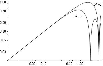
From the last part of (4.11) we see that for differentiation with fixed order the first term gives the characteristic function of the ideal differentiator. The second term has degree in and gives rise to a falling down of the characteristic function, since the coefficient has negative sign. So for high frequencies the filter will be a low pass filter and for low frequencies the filter works well for differentiation. Increase of brings the filter in a sense closer to the ideal differentiator (see also Remark 4.4 for approximation to in the -domain), but the pass band will also increase, causing more high frequency noise (see section 5.2 and Figure 1 for an example in the Legendre case). In the practice of the construction of a differentiating filter one has to decide to what frequency the differentiation must do the job and how much noise one accepts. This all depends on the frequency contents of the signal and the noise. See also the discussion for the case of constant weights by Barak [5, p.2761] (for ) and by Luo et al. [44, §5] (for general ).
4.4 Smoothing filters
For the filters given by the left-hand sides of (4.1) and (4.6) are examples of smoothing filters. These have a very long history, see Schoenberg [58], [59] and references given there, which go back as far as De Forest’s work in 1878. We put in (4.7) and in (4.8):
| (4.12) | ||||
| (4.13) |
and we usually take symmetric: .
We say that (4.12) or (4.13) is exact for the degree (where in case of (4.12)) if whenever is a polynomial of degree , but for some polynomial of degree . Because of symmetry of , such will always be odd.
Exactness of (4.12) for degree at least can equivalently be stated as
with
where is a Gram polynomial (see (2.4)) and is the corresponding constant given by (2.6). For such the sum of squares is minimal if and only if for . Then
| (4.14) |
where is the Christoffel-Darboux kernel of degree (see (2.14)) for the orthogonal polynomials .
Similarly, in case of (4.13) and assuming that is a polynomial, the requirements that the formula is exact for the degree and that is minimal are equivalent to
| (4.15) |
where is the Christoffel-Darboux kernel of degree for the Legendre polynomials .
More generally than (4.14) we can work with orthogonal polynomials satisfying (2.2) or (2.3) for equidistant points running over a symmetric set and with symmetric weights:
where . In terms of these polynomials exactness of (4.12) for degree at least can equivalently be stated as
| (4.16) |
with
| (4.17) |
In particular, the choice
| (4.18) |
with the Christoffel-Darboux kernel and with (2.15) used for the second equality, will make (4.12) exact for the degree .
The characteristic function for (4.12) respectively (4.13) is defined by (4.9) with respectively (4.10) with . The condition that (4.12) or (4.13) is exact for the degree is equivalent with the condition that has power series of the form
| (4.19) |
with .
An -fold iteration of (4.12) (with for convenience) yields
where is an -fold convolution product. De Forest (1878) raised the question for which choices of the asymptotic behaviour of for large can be described. Schoenberg [58, Theorem 1 and Remark 1 on p.358] showed that this is possible precisely if the characteristic function satisfies
| (4.20) |
If (4.20) is satisfied then the smoothing is called stable. Clearly (4.20) will imply that (4.19) holds with . For given by (4.18) we see from (4.11) that is satisfied for any choice of the weights and that is explicitly given by
4.5 Fourier-Bessel functions
As a common generalization of (4.12) and (4.13) with given by (4.15) and (4.18), respectively, we can consider a smoothing formula
| (4.21) |
with an even positive orthogonality measure for the orthogonal polynomials and with given by
| (4.22) |
(Such usage of the Christoffel-Darboux formula was emphasized in [53] for the cases of Gram and Legendre polynomials.) Then we can define the corresponding characteristic function by
| (4.23) | ||||
Thus
| (4.24) |
In the Legendre case with support we can evaluate integrals occurring above in terms of (spherical) Bessel functions as follows:
| (4.25) |
see [50, (18.17.19), (10.47.3)] or [6, (4)]. In the Chebyshev case , we similarly obtain (see [50, (10.9.2)])
| (4.26) |
Formula (4.26) was the reason for Mantica [45], [46] to call the functions
| (4.27) |
Fourier-Bessel functions (where he took orthonormal and a probability measure). The same functions occur in Ignjatović [34] as the functions (in the notation of [34, §2.1]). Formula (4.25) played an important role in the proof of the stability result in the Legendre case, see [43]. It also occurred in Rangarajan et al. [54, (14), (15)] for a formal operational calculus in connection with the right-hand side of (3.6) before taking limits. In the Appendix we will compute the Fourier-Bessel functions for the case of the shifted symmetric Hahn polynomials (4.28).
4.6 Stability of smoothing in case of symmetric Hahn and Krawtchouk polynomials
The shifted symmetric Hahn polynomials
| (4.28) |
are orthogonal polynomials on with respect to the symmetric weights
| (4.29) |
see [36, (9.5.1) and (9.5.2)]. Assume that is a nonnegative integer. Consider in terms of these polynomials formulas (4.16) and (4.17) characterizing exactness for degree at least . Now observe that, by [36, (9.5.9)], we have
where . It follows that
| (4.30) |
is minimal for given by (4.16) and (4.17) if and only if for . Greville [24, §3] (1966) denotes (4.30) by (after division by ). Therefore he calls the smoothing formula (4.12) the minimum formula if is taken such that (4.30) is minimal. Greville [24, (4.2)] gives an explicit formula for the characteristic function in case of a minimum formula. He ascribes this formula to Sheppard [61] (1913). We will derive this formula in the Appendix. Greville [24, §5] next proves the stability property (4.20) for these cases. Curiously, Greville does not mention Hahn polynomials in any way. Hahn polynomials in this context seem to come up first in Bromba & Ziegler [7, §3.2].
As a special case of [36, (9.5.16)] there is the limit formula
| (4.31) |
where the polynomials are Krawtchouk polynomials (see [36, §9.11]). The corresponding weights (4.29), suitably normalized, tend for to the symmetric weights
with respect to which the polynomials are orthogonal. The smoothing formula with given by (4.18) for this and is called the minimum formula by Greville [24, §6]. He obtains the characteristic function for this case explicitly as a limit case of his formula in the minimum case (see also (A.9)), not working with Krawtchouk polynomials at all. (Krawtchouk polynomials seem to come up first in this context in Bromba & Ziegler [7, §3.3].) But Greville also obtains in some way that,
| (4.32) |
Let us prove this by observing from (4.31) that
Hence
for by orthogonality. Now Greville concludes from (4.19) and (4.32) that
| (4.33) |
for certain polynomials of degree and of degree . From that he immediately derives that is equal to the power series of truncated after the term with , i.e.,
| (4.34) |
By a similar argument we see that
| (4.35) |
Hence, by (4.33),
which is even stronger than the stability condition (4.20).
Identity (4.33) with and given by (4.34), (4.35) has a long history which is surveyed in Koornwinder & Schlosser [39]. However, this paper missed Greville’s paper and the connection with Krawtchouk polynomials. A sequel [40] to [39], tracing (4.33)–(4.35) back to 1713, has appeared.
By a short chain of identities, using (4.33) and (4.34), can be expressed as
see [39, top of p.249]. Hence is monotonically decreasing on from 1 to 0. Such filters without ripples are called maximally flat by Herrmann [31] (see also Samadi and Nishihara [56]). Herrmann gave the same argument as above for solving (4.33), apparently unaware of Greville [24].
4.7 The Savitzky-Golay paper and its follow-up
The first instance of an approximation of first and higher derivatives by formula (4.1) with possibly was given by Savitzky & Golay [57] in 1964. They only dealt with the case of constant weights on , they used only very special , and , and they did not explicitly mention or use the corresponding orthogonal polynomials. They were motivated by applications in spectroscopy. Their paper had an enormous impact, for instance 5432 citations in Google Scholar in January 2012. Some corrections to [57] were given by Steinier et al. [62] in 1972.
Probably, Gorry [22] (1990) was the first who gave (4.1) in a more structural form in the case of constant weights on an equidistant set using centered Gram polynomials. Next, in [23] (1991) he considered (4.1) on a finite non-equidistant set, still with constant weights. Meer & Weiss [47] (1992) gave (4.1) for orthogonal polynomials on a set with respect to general weights. They made this more explicit in the cases of centered Gram polynomials and of centered Krawtchouk polynomials with symmetric weights.
We recommend Luo et al. [44] as a relatively recent survey of follow-up to the Savitzky-Golay paper.
5 Filter properties in the frequency domain: some examples
In section 4 many so-called linear filters for derivatives were mentioned. In electrical engineering one uses the transfer function for understanding the properties of the filter. This is the Fourier transform of the unit impulse response of the filter, see (4.9), (4.10) where we wrote instead of . In general, this function is complex-valued. We can show the properties of the filter in the frequency domain by a log-log plot of the modulus of the transfer function (which may be complemented by a phase plot). In general, for a differentiation filter of order , should behave for low frequencies like , and for high frequencies like a constant (equal to zero in the ideal case). When the behaviour is different, the filter is called unstable.
5.1 The Lanczos derivative
The (analog) filter corresponding to the Lanczos derivative is given by (3.7) ignoring the limit:
| (5.1) |
The output function can be considered as a continuous (i.e. unsampled) approximation of the first derivative of the input function . The transfer function is equal to the quotient of and with . A short computation gives
| (5.2) | ||||
compatible with (4.11) for , . For small we have . The modulus of for is given in Figure 1, case as a log-log plot.
5.2 Multi-term variant of the Lanczos derivative
To get a better approximation we can use equation (4.1) with a Legendre polynomial:
| (5.3) |
Here
by [18, 10.10(26), 10.9(19)] and (2.10). For (5.3) reduces to (5.1). For the transfer function we obtain (see also (4.11)):
where the spherical Bessel functions entered by (4.25). An explicit formula for spherical Bessel functions is given in [50, (10.49.2)]. In particular,
Thus is given by (5.2). After some computation we obtain
| (5.4) |
The modulus of for is also given in figure 1, case . It is clear that for the plot stays close to a straight line until higher values of than for .

5.3 First order Savitzky-Golay filter
When the input signal of the filter is given by a vector of (for convenience) odd dimension obtained by sampling a function on equidistant points , then we may use (3.4) ignoring the limit as a discrete filter for the -th derivative of at . In particular, for , we can use (3.5):
For the transfer function
| (5.5) |
we obtain by straightforward computation that
| (5.6) |
Note that the phase shift is exactly .
5.4 Butterworth filter
If one needs a filter that does differentiation for low frequencies very well and has a good suppression for high frequencies then there are better filters than the ones discussed in this paper until here. For example there are the so-called Tchebyshev, inverse Tchebyshev, Elliptic, Butterworth and Bessel filters. These filters all differentiate, but the choice of the most suitable filter depends on the properties one needs, for instance a constant phase response, a good amplitude response, less side-lobes etc. We mention here the so-called -th order Butterworth filter. The square of the modulus of the transfer function of an -th order analog Butterworth filter that differentiates with order is given by
| (5.7) |
Here is the so-called cutoff frequency. It is at this frequency where the the asymptotics of the low frequency part and the high frequency part of the transfer function meet. The factor is the square of the modulus of the transfer function of the ideal -th order differentiator.
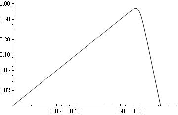
As an example see Figure 3 showing the transfer function of a seventh order Butterworth filter with (see how the side lobes differ from those of Figure 2).
In (5.7) one has to make a choice of as follows:
such that is a polynomial of degree with real coefficients for which all (possibly complex) roots have negative real part. Then (4.10) and (4.8) take the form
is called the impulse response of the filter. It follows that the output function satisfies a differential equation with the input function as inhomogeneous part:
For instance, for we have
For we have
One can obtain the transfer function for the Butterworth filter in the digital case from in the analog case by so-called frequency warping: replace by , where is the length of the sampling interval. Then some linear combination of finitely many output values will be equal to some linear combination of finitely many input values (a so-called recursive filter).
There are important differences for practical applications between filters obtained from orthogonal polynomials, as amply considered in this paper, and the Butterworth filter. In the analog case the Butterworth filter can be much easier constructed physically. But in the discrete case the filters obtained from orthogonal polynomials are much easier to handle in the time domain than the Butterworth filter.
Appendix A Appendix
Here we derive an explicit expression for the Fourier-Bessel functions (see (4.27)) associated with the shifted symmetric Hahn polynomials (see (4.28)). First observe that by the duality between Hahn polynomials and dual Hahn polynomials (see the formula after (9.6.16) in [36]) the generating function [36, (9.6.12)] for dual Hahn polynomials can be rewritten in terms of Hahn polynomials:
| (A.1) |
where
| (A.2) |
i.e., the weight occurring in the orthogonality relation [36, (9.5.2)] for Hahn polynomials.
Now use the quadratic transformation [17, 2.11(30)] and the expression [18, 10.9(20)] of Gegenbauer polynomials in terms of hypergeometric functions:
Thus we can rewrite (A.3) as
| (A.4) |
The left-hand side of (A.4) gives an expression for the Fourier-Bessel function (4.27) associated with the shifted symmetric Hahn polynomials (4.28).
Now let be defined by (4.23), (4.22) with given by (4.28). Then combination of (4.24), (A.4) and [18, 10.9(22)] yields that
| (A.5) |
where
| (A.6) |
In the last equality we used [36, (9.5.2), (9.5.4)] for and and [15, (2.4)] together with [36, (9.5.3)] for getting
| (A.7) |
Formulas (A.5), (A.6) coincide with formulas (4.3), (4.4) in Greville [24] if we replace by , respectively. Integration of (A.6) together with yields
| (A.8) |
Formula (A.8) coincides with formula (4.2) in Greville [24], which Greville (in his earlier form (4.1)) ascribes to Sheppard [61]. However, we have only been able to find a match of the special case of [24, (4.1)] with a formula in Sheppard’s paper, namely with [61, (64)].
In the limit for formula (A.8) becomes
| (A.9) |
This coincides with the formula after (6.1) in Greville [24], and also with (4.33) combined with (4.35) and [1, (2.3.15)].
If then the left-hand side of (A.4) can be written as a finite sum, where the number of terms is independent of . First observe that by [50, (14.13.1), (14.3.21), (5.5.5)] we have
| (A.10) |
For the above series terminates after the term with . Hence, for (A.4) takes the form
| (A.11) |
For and formula (A.11) specializes to (5.6) with given by (5.5). Use that .
References
- [1] G. E. Andrews, R. Askey and R. Roy, Special Functions, Cambridge University Press, 1999.
- [2] A. Antonio, Digital Filters, McGraw-Hill, second ed., 1993.
- [3] T. Apostol, Calculus, Vol. 1, Wiley, second ed., 1967.
- [4] R. Askey and D. T. Haimo, Similarities between Fourier and power series, Amer. Math. Monthly 103 (1996), 297–304.
- [5] Ph. Barak, Smoothing and differentiation by an adaptive-degree polynomial filter, Anal. Chem. 67 (1995), 2758–2762.
- [6] J. A. Barcelo and A. Córdoba, Band-limited functions: -convergence, Trans. Amer. Math. Soc. 313 (1989), 655–669.
- [7] M. U. A. Bromba and H. Ziegler, On Hilbert space design of least-weighted-squares digital filters, Internat. J. Circuit Theory Appl. 11 (1983), 7–32.
- [8] N. Burch, P. E. Fishback and R. Gordon, The least-squares property of the Lanczos derivative, Math. Mag. 78 (2005), 368–378.
- [9] N. Burch and P. E. Fishback, Orthogonal polynomials and regression-based symmetric derivatives, Real Anal. Exchange 32 (2007), 597–607.
- [10] P. L. Chebyshev, On the interpolation of equidistant values (in Russian), Peters. Gel. Anz. 25 (1873); translated in French in Oeuvres de P. L. Chebyshev (A. Markoff and N. Sonin, eds., St. Petersburg, 1899/1907), Vol. 2, pp. 217–242; reprinted Chelsea, N.Y., 1962.
- [11] N. Cioranescu, La généralisation de la première formule de la moyenne, Enseign. Math. 37 (1938), 292–302.
- [12] A. Cohen and I. Daubechies, A new technique to estimate the regularity of refinable functions, Rev. Mat. Iberoamericana 12 (1996), 527–591.
- [13] I. Daubechies, Orthonormal bases of compactly supported wavelets, Comm. Pure Appl. Math. 41 (1988), 909–996.
- [14] I. Daubechies, Ten lectures on wavelets, SIAM, 1992.
- [15] E. Diekema and T. H. Koornwinder, Generalizations of an integral for Legendre polynomials by Persson and Strang, J. Math. Anal. Appl. 388 (2012), 125–135; arXiv:1005.2285v2 [math.CA].
- [16] J. Dutka, On Gauss’ priority in the discovery of the method of least squares, Arch. Hist. Exact Sci. 49 (1996), 355–370.
- [17] A. Erdélyi, Higher transcendental functions, Vol. I, McGraw-Hill, 1953.
- [18] A. Erdélyi, Higher transcendental functions, Vol. II, McGraw-Hill, 1953.
- [19] A. Fischer, Differentiability of Peano derivatives, Proc. Amer. Math. Soc. 136 (2008), 1779–1785.
- [20] P. Fishback, Taylor series are limits of Legendre expansions, Missouri J. Math. Sci. 19 (2007), 29–34.
- [21] R. A. Gordon, Peano differentiation via integration, Real Anal. Exchange 34 (2009), 147–156.
- [22] P. A. Gorry, General least-squares smoothing and differentiation by the convolution (Savitzky-Golay) method, Anal. Chem. 62 (1990), 570–573.
- [23] P. A. Gorry, General least-squares smoothing and differentiation of nonuniformly spaced data by the convolution method, Anal. Chem. 63 (1991), 534–536.
- [24] T. N. E. Greville, On stability of linear smoothing formulas, SIAM J. Numer. Anal. 3 (1966), 157–170.
- [25] C. W. Groetsch, Lanczos’ generalized derivative, Amer. Math. Monthly 105 (1998), 320–326.
- [26] R. W. Hamming, Numerical methods for scientists and engineers, second ed., Dover Publications, 1986.
- [27] R. W. Hamming, Digital filters, third ed., Dover Publications, 1989.
- [28] G. H. Hardy, A course of pure mathematics, Cambridge University Press, tenth ed., 1952.
- [29] U. S. Haslam-Jones, On a generalized derivative, Quart. J. Math, Oxford Ser. (2) 4 (1953), 190–197.
- [30] C. Herley and M. Vetterli, Wavelets and recursive filter banks, IEEE Trans. Signal Process. 41 (1993), 2536–2556.
- [31] O. Herrmann, On the approximation problem in nonrecursive digital filter design, IEEE Trans. Circuit Theory 18 (1971), 411–413.
- [32] D. L. Hicks and L. M. Liebrock, Lanczos’ generalized derivative: insights and applications, Appl. Math. Comput. 112 (2000), 63–73
- [33] F. B. Hildebrand, Introduction to numerical analysis, Dover Publications, 1974.
- [34] A. Ignjatović, Local approximations based on orthogonal differential operators, J. Fourier Anal. Appl. 13 (2007), 309–330.
- [35] D. E. Johnson, Introduction to filter theory, Prentice-Hall, 1976.
- [36] R. Koekoek, P. A. Lesky and R. F. Swarttouw, Hypergeometric orthogonal polynomials and their -analogues, Springer-Verlag, 2010.
- [37]
T. H. Koornwinder,
Orthogonal polynomials with weight function
, Canad. Math. Bull. 27 (1984), 205–214. - [38] T. H. Koornwinder, The continuous wavelet transform, in Wavelets: an elementary treatment of theory and applications, World Scientific, 1993, pp. 27–48.
- [39] T. H. Koornwinder and M. J. Schlosser, On an identity by Chaundy and Bullard. I, Indag. Math. (N.S.) 19 (2008), 239–261.
- [40] T. H. Koornwinder and M. J. Schlosser, On an identity by Chaundy and Bullard. II. More history, Indag. Math. (N.S.) 24 (2013), 174–180.
- [41] D. Kopel and M. Schramm, A new extension of the derivative, Amer. Math. Monthly 97 (1990), 230–233.
- [42] C. Lanczos, Applied analysis, Prentice-Hall, 1956.
- [43] L. Lorch and P. Szego, A Bessel function inequality connected with stability of least square smoothing. II, Glasgow Math. J. 9 (1968), 119–122.
- [44] J. Luo, K. Ying. P. He and J. Bai, Properties of Savitzky-Golay digital differentiators, Digital Signal Processing 15 (2005), 122–136.
- [45] G. Mantica, Generalized Bessel functions: theoretical relevance, and computational techniques, in Self-similar systems, Joint Inst. Nuclear Res., Dubna, 1999, pp. 306–315.
- [46] G. Mantica, Fourier-Bessel functions of singular continuous measures and their many asymptotics, Electron. Trans. Numer. Anal. 25 (2006), 409–430.
- [47] P. Meer and I. Weiss, Smoothed diferentiation filters for images, J. Visual Comm. Image Repr. 3 (1992), 58–72.
- [48] M. Moncayo and R. J. Yáñez, Continuous wavelet transforms based on classical orthogonal polynomials and functions of the second kind, J. Comput. Anal. Appl. 9 (2007), 207–220.
- [49] A. F. Nikiforov, S. K. Suslov and V. B. Uvarov, Classical orthogonal polynomials of a discrete variable, Springer-Verlag, 1991.
- [50]
NIST Handbook of Mathematical Functions,
Cambridge University Press, 2010;
http://dlmf.nist.gov. - [51] A. V. Oppenheim and R. W. Schafer, Digital signal processing, Prentice Hall, 1975.
- [52] G. Peano, Sulla formula di Taylor, Torino Atti 27 (1891), 40–46.
- [53]
P.-E. Persson and G. Strang,
Smoothing by Savitzky-Golay and Legendre filters, in
Mathematical systems theory in biology, communications, computation, and finance,
IMA Vol. Math. Appl. 134, 2003, pp. 301–316. - [54] S. K. Rangarajan and S. P. Purushothaman, Lanczos’ generalized derivative for higher orders, J. Comput. Appl. Math. 177 (2005), 461–465.
- [55] A. Rieder, The high frequency behaviour of continuous wavelet transforms, Appl. Anal. 52 (1994), 125–141.
- [56] S. Samadi and A. Nishihara, The world of flatness, IEEE Circuits Systems Magazine 7 (2007), 38–44.
- [57] A. Savitzky and M. J. E. Golay, Smoothing and differentiation of data by simplified least squares procedures, Anal. Chem. 36, 1964, 1627–1639.
- [58] I. J. Schoenberg, Some analytical aspects of the problem of smoothing, in Studies and Essays Presented to R. Courant on his 60th Birthday, January 8, 1948, Interscience, 1948. pp. 351–370.
- [59] I. J. Schoenberg, On smoothing operations and their generating functions, Bull. Amer. Math. Soc. 59 (1953), 199–230.
- [60] J. Shen, On the generalized “Lanczos’ generalized derivative”, Amer. Math. Monthly 106 (1999), 766–768.
- [61] W. F. Sheppard, Reduction of errors by means of negligible differences, Proceedings International Congress of Mathematicians, Cambridge, Vol. 2, 1912, 348–384.
- [62] J. Steinier, Y. Termonia and J. Deltour, Smoothing and differentiation of data by simplified least square procedure, Anal. Chem. 44 (1972), 1906–1909.
- [63] F. Strik, Ophthalmodynamographie und Ophthalmodynamometrie in der neurologischen Praxis, Dissertation, Erasmus Universiteit Rotterdam, 1977.
- [64] G. Szegő, Orthogonal polynomials, Amer. Math. Soc. Colloquium Publications 23, Amer. Math. Soc., Fourth ed., 1975.
- [65] W. F. Trench, On the stability of midpoint smoothing with Legendre polynomials, Proc. Amer. Math. Soc. 18 (1967), 191–199.
- [66]
L. Washburn, The Lanczos’ derivative,
Senior project, Whitman College, 2006;
https://www.whitman.edu/Documents/Academics/Mathematics/washbuea.pdf.
E. Diekema, Kooikersdreef 620, 7328 BS Apeldoorn, The Netherlands;
email: e.diekema@gmail.com
T. H. Koornwinder, Korteweg-de Vries Institute, University of
Amsterdam,
P.O. Box 94248, 1090 GE Amsterdam, The Netherlands;
email: thkmath@xs4all.nl