跳到论文正文
W Papers独立论文阅读器 arXiv:1102.5138 论文正文 计算阅读时间 · 0%
引用这篇论文根据当前论文元数据生成,正式投稿前建议核对。


License: arXiv.org perpetual non-exclusive license
arXiv:1102.5138v1 [cs.IT] 25 Feb 2011

Low-Complexity Near-Optimal Codes
for Gaussian Relay Networks

Affiliation: Theodoros K. Dikaliotis Affiliation: Hongyi Yao Affiliation: A. Salman Avestimehr Affiliation: Sidharth Jaggi Affiliation: Tracey Ho
 California Institute of Technology  Cornell University  Chinese University of Hong Kong
{tdikal, tho}@caltech.edu  yaohongyi03@gmail.com  avestimehr@ece.cornell.edu  jaggi@ie.cuhk.edu.hk
Abstract

We consider the problem of information flow over Gaussian relay networks. Similar to the recent work by Avestimehr et al. [1], we propose network codes that achieve up to a constant gap from the capacity of such networks. However, our proposed codes are also computationally tractable. Our main technique is to use the codes of Avestimehr et al. as inner codes in a concatenated coding scheme.

I Introduction

The recent work of [1] parallels the classical network coding results [2] for wireless networks. That is, it introduces a quantize-map-and-forward scheme that achieves all rates up to a constant gap to the capacity of Gaussian relay networks, where this constant depends only on the network size, and varies linearly with it. However the computational complexity of encoding and decoding for the codes of [1] grows exponentially in the block-length.

In this work, we aim to construct low complexity coding schemes that achieve to within a constant gap of the capacity of Gaussian relay networks. The simplest Gaussian network that has been well investigated in the coding literature is the point-to-point Additive White Gaussian Noise (AWGN) channel. There have been a variety of capacity achieving codes developed for such channels (see e.g., [3, 4, 5, 6] and references therein).

There have also been several recent efforts (for instance [7] and  [8]) to extend the result of  [1] and build low complexity relaying strategies that achieve up to a constant gap from the capacity of Gaussian relay networks. However the decoding complexity of the proposed codes is still exponential in the block-length. This is because these strategies are based on lattice codes, in which decoding proceeds via nearest neighbour search, which in general is computationally intractable.

In this paper, we build a coding scheme that has computational complexity that is polynomial in the block-length11 1 The computational complexity of all existing codes, such as in [1], also grow exponentially in network parameters, namely the number of nodes |𝒩||\mathcal{N}|. In fact, the codes proposed in this work have the same property. However, for our purposes we consider the network size to be fixed and small. and achieves rates up to a constant gap to the capacity of Gaussian relay networks.

More specifically, we build a Forney-type [9] two-layered concatenated code construction for Gaussian relay networks. As our inner codes we use improved versions of the inner code in  [1], which can be decoded with probability of error dropping exponentially fast in the inner code block-length. As our outer codes we use polar codes [10], which are provably capacity achieving (asymptotically in their block-lengths) for the Binary Symmetric Channel, and have computational complexity that is near-linear in their block-lengths.

II Model

We consider an additive white Gaussian noise (AWGN) relay network 𝒢=(𝒩,ℰ)\mathcal{G}=\left(\mathcal{N},\mathcal{E}\right), where 𝒩\mathcal{N} denotes the set of nodes and ℰ\mathcal{E} the set of edges between nodes. Within the network there is a source 𝒮∈𝒩\mathcal{S}\in\mathcal{N} and a sink node22 2 Just as in wired network coding, this result extends directly to the case of multiple sinks – to ease notational burden we focus on the case of a single sink. ℛ∈𝒩\mathcal{R}\in\mathcal{N} where the source has a set of messages it tries to convey to the sink. For every node i∈𝒩i\in\mathcal{N} in the network there is the set ℐi={j∈𝒩:(j,i)∈ℰ}⊆𝒩\mathcal{I}_{i}=\{j\in\mathcal{N}:(j,i)\in\mathcal{E}\}\subseteq\mathcal{N} of nodes that have edges incoming to node ii. All nodes have a single receiving and transmitting antenna and the received signal yi,ty_{i,t} at node ii at time tt is given by

yi,t=∑j∈ℐihj​i​xj,t+zi,t\displaystyle y_{i,t}=\sum_{j\in\mathcal{I}_{i}}h_{ji}x_{j,t}+z_{i,t} (1)

where xj,t∈ℂx_{j,t}\in\mathbb{C} the signal transmitted from node jj at time tt and hj​i∈ℂh_{ji}\in\mathbb{C} is the channel gain associated with the edge connecting nodes jj and ii. The receiver noise, zi,tz_{i,t}, is modeled as a complex Gaussian random variable 𝒞​𝒩​(0,1)\mathcal{CN}(0,1), with i.i.d. distribution across time. Further we assume that there is an average transmit power constraint equal to 11 at each node in the network.

Without loss of generality we assume that network 𝒢\mathcal{G} has a layered structure, i.e., all paths from the source to the destination have equal length. The number of layers in 𝒢\mathcal{G} is denoted by L𝒢L_{\mathcal{G}}, and the source 𝒮\mathcal{S} resides at layer 11 whereas the sink ℛ\mathcal{R} is at layer L𝒢L_{\mathcal{G}}. As in Section VI-B of  [1] the results of this paper can be extended to the general case by expanding the network over time since the time-expanded network is layered.

III Transmission Strategy and Main Result
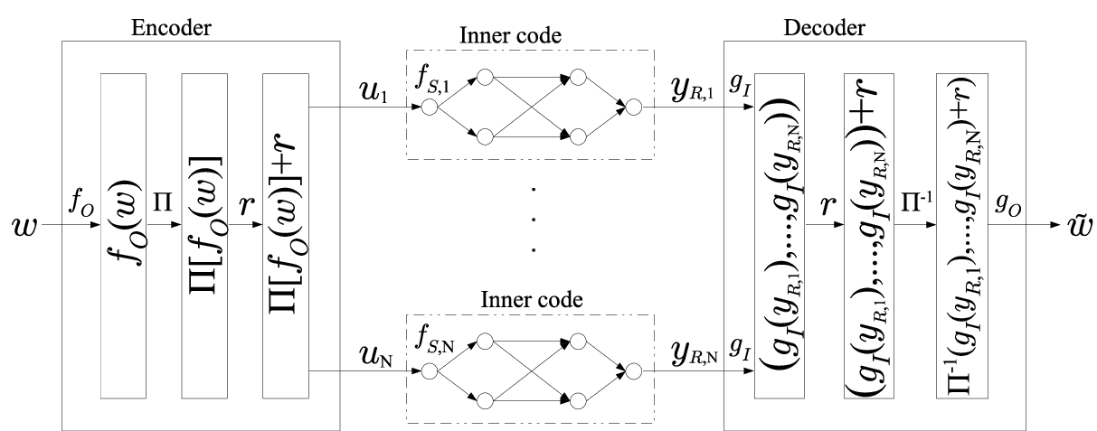
Refer to caption
Fig. 1: System diagram of our concatenated code design.

Our source encoder operates at two levels, respectively the outer code level and the inner code level. The outer code we use is a polar code [11] (along with a random permutation of bits passed from the outer code to the encoders for the inner code – this permutation is used for technical reasons that shall be described later). The inner code is a random code similar to the inner code used in [1]. The relay nodes use “quantize-map-and-forward” as in [1] over a short block-length (i.e., the block-length of the inner code). Finally the receiver decodes the inner coding operations, inverts the random permutation inserted by the source encoder, and finally decodes the corresponding outer polar code.

The reason for using a two-layered concatenated code is to achieve both low encoding and decoding complexity, and a decoding error probability that decays almost exponentially fast with the block-length. In particular, as we describe in Section  IV, our inner codes have a decoding algorithm that is based on exhaustive search. To ensure our inner codes’ decoding complexity is tractable we set the block-length of the inner codes to be a “relatively small” fixed value. As a result, the decoding error probability for our inner codes is also fixed. To circumvent this, we then add an outer code on top of the inner code. More specifically, we use a polar code as an outer code, since polar codes have many desirable properties – in particular, they provably have encoding and decoding complexities that are near linear in the block-length, are asymptotically capacity achieving, and also have probability of error that decays nearly exponentially in the block-length  [11].

One technical challenge arises. Polar codes are capable of correcting independent bit flips, but are not guaranteed to work against bursts of consecutive bit flips. It is to “spread out” the possibly correlated bit-flips that would occur if one or several inner codes decode incorrectly that we introduce the random permutation mentioned above to the output of the source encoder’s outer polar code. This random permutation is based on public randomness, and hence is available to both the source encoder, and the sink decoder (which can therefore invert it). The system diagram of our coding scheme is shown in Figure  1. We now describe the details of the encoding, relaying, and decoding operations used by the source, relay nodes and the sink. Also, the source outer code encoder XORs a random string (denoted rr, and known in advance to all parties via public randomness) to its output after permuting the bits of the polar code, but before passing these bits to the inner codes. This is to ensure independence of the inputs to the inner codes, so that concentration results can be used.

III-A Encoding at the Source and the Relays

The overall communication scheme is over nn time instants and has a rate of R=RO​RIR=R_{O}R_{I}, where ROR_{O} and RIR_{I} are the rates for the outer code, and each of the inner codes, respectively. The source takes a message 𝐰∈𝔽2RO​RI​n\mathbf{w}\in\mathbb{F}_{2}\hskip-2.84526pt^{R_{O}R_{I}n} of size RO​RI​nR_{O}R_{I}n bits, and first applies the encoding algorithm of the polar code fO:𝔽2RO​RI​n→𝔽2RI​nf_{O}:\mathbb{F}_{2}\hskip-2.84526pt^{R_{O}R_{I}n}\rightarrow\mathbb{F}_{2}\hskip-2.84526pt^{R_{I}n} creating a string fO​(𝐰)∈𝔽2RI​nf_{O}(\mathbf{w})\in\mathbb{F}_{2}\hskip-2.84526pt^{R_{I}n} of RI​nR_{I}n bits. Once the vector fO​(𝐰)f_{O}(\mathbf{w}) is formed a random permutation Π\Pi is applied on all the bits of fO​(𝐰)f_{O}(\mathbf{w}) giving rise to Π⁡[fO​(𝐰)]∈𝔽2RI​n\Pi\left[f_{O}(\mathbf{w})\right]\in\mathbb{F}_{2}\hskip-2.84526pt^{R_{I}n}. A random length-RI​nR_{I}n bit-vector rr is then XORed with Π⁡[fO​(𝐰)]∈𝔽2RI​n\Pi\left[f_{O}(\mathbf{w})\right]\in\mathbb{F}_{2}\hskip-2.84526pt^{R_{I}n}.

The derived bit-vector Π​[fO​(𝐰)]\Pi\left[f_{O}(\mathbf{w})\right] is divided in N=nℓN=\frac{n}{\ell}, i.e. Π⁡[fO​(𝐰)]=(𝐮1,…,𝐮N)\Pi\left[f_{O}(\mathbf{w})\right]=\left(\mathbf{u}_{1},\ldots,\mathbf{u}_{N}\right), chunks of size RI​ℓR_{I}\ell bits, i.e. 𝐮k∈𝔽2RI​ℓ\mathbf{u}_{k}\in\mathbb{F}_{2}\hskip-2.84526pt^{R_{I}\ell} for 1≤k≤N1\leq k\leq N. Each one of the bit-vectors 𝐮k\mathbf{u}_{k} is conveyed through the network independently using a separate random inner code of rate RIR_{I} and block-length ℓ\ell introduced in [1].

More specifically, all nodes in the network operate over blocks of length ℓ\ell. The source randomly maps each inner code symbol 𝐮k∈{1,…,2RI​ℓ}\mathbf{u}_{k}\in\{1,\ldots,2^{R_{I}\ell}\} to a transmitted vector of length ℓ\ell with components distributed i.i.d. from 𝒞​𝒩​(0,1)\mathcal{CN}(0,1). That is, for each 1≤k≤N1\leq k\leq N the random inner codes operate as F𝒮,k:{1,2,…,2RI​ℓ}→ℂℓF_{\mathcal{S},k}:\left\{1,2,\ldots,2^{R_{I}\ell}\right\}\rightarrow\mathbb{C}\hskip 1.42262pt^{\ell}, where realizations of F𝒮,kF_{\mathcal{S},k} are denoted f𝒮,kf_{\mathcal{S},k}. For each 1≤k≤N1\leq k\leq N, each relay node i∈𝒢i\in\mathcal{G} rounds the real and imaginary part of each component of its received vector 𝐲i,k∈ℂℓ\mathbf{y}_{i,k}\in\mathbb{C}\hskip 1.42262pt^{\ell} to the closest integer to form the length-ℓ\ell vector ([𝐲i,k][\mathbf{y}_{i,k}]). It then randomly maps [𝐲i,k][\mathbf{y}_{i,k}] it to a transmit vector of length ℓ\ell with components distributed i.i.d. from 𝒞​𝒩​(0,1)\mathcal{CN}(0,1). For each 1≤k≤N1\leq k\leq N the mappings at relay i∈𝒩i\in\mathcal{N} are denoted by Fi,k:(𝒜iℓ,𝒜iℓ)→ℂℓF_{i,k:}\left(\mathcal{A}_{i}^{\ell},\mathcal{A}_{i}^{\ell}\right)\rightarrow\mathbb{C}\hskip 1.42262pt^{\ell}, with fi,kf_{i,k} denoting a specific realization of Fi,kF_{i,k}. Here 𝒜i={−si,…,si}\mathcal{A}_{i}=\{-s_{i},\ldots,s_{i}\} is the set of integers from −si-s_{i} to sis_{i}, where sis_{i} is a code design parameter be specified later. If the incoming signal at a relay node has a component such that its real or imaginary part is larger than sis_{i} in magnitude then an error is declared. Finally, the sink ℛ\mathcal{R} receives 𝐲ℛ,k∈ℂℓ\mathbf{y}_{\mathcal{R},k}\in\mathbb{C}\hskip 1.42262pt^{\ell} associated with inner code symbol 𝐮k\mathbf{u}_{k}.

III-B Decoding

At the end of the transmission scheme, sink ℛ\mathcal{R} receives 𝐲ℛ∈ℂn\mathbf{y}_{\mathcal{R}}\in\mathbb{C}\hskip 1.42262pt^{n}, which consists of NN chunks of length ℓ\ell, i.e. 𝐲ℛ=(𝐲ℛ,1,…,𝐲ℛ,N)\mathbf{y}_{\mathcal{R}}=\left(\mathbf{y}_{\mathcal{R},1},\ldots,\mathbf{y}_{\mathcal{R},N}\right) where 𝐲ℛ,k∈ℂℓ\mathbf{y}_{\mathcal{R},k}\in\mathbb{C}\hskip 1.42262pt^{\ell}. For each chunk 𝐲i,k\mathbf{y}_{i,k}, 1≤k≤N1\leq k\leq N, the sink ℛ\mathcal{R} then applies the decoding algorithm gI:ℂℓ→2RI​ℓg_{I}:\mathbb{C}\hskip 1.42262pt^{\ell}\rightarrow 2^{R_{I}\ell} of the corresponding inner code (to be described in Section  IV). The sink then obtains 𝐮^k\hat{\mathbf{u}}_{k}, a possibly noisy version of the corresponding inner code length-ℓ\ell bit-vector 𝐮k\mathbf{u}_{k} that was transmitted during the kthk^{\text{th}} application of the inner code. After decoding all chunks, it then XORs out the random bit-string rr added as part of the encoding procedure and then the inverse of the permutation applied by the source encoder is applied, i.e. Π−1​[(gI​(𝐲ℛ,1),…,gI​(𝐲ℛ,N))]\Pi^{-1}\left[\left(g_{I}(\mathbf{y}_{\mathcal{R},1}),\ldots,g_{I}(\mathbf{y}_{\mathcal{R},N})\right)\right]. Finally, the sink utilizes the polar code decoder in order to produce the estimate for the source message, i.e. 𝐰~=gO​(Π−1​[(gI​(𝐲ℛ,1),…,gI​(𝐲ℛ,N))])\tilde{\mathbf{w}}=g_{O}\left(\Pi^{-1}\left[\left(g_{I}(\mathbf{y}_{\mathcal{R},1}),\ldots,g_{I}(\mathbf{y}_{\mathcal{R},N})\right)\right]\right). An error is declared if 𝐰≠𝐰~{\mathbf{w}}\neq\tilde{\mathbf{w}}.

III-C Main Result

As in [1] we define C¯\bar{C} to be the cut-set upper bound on the capacity CC of a general Gaussian relay network, i.e.,

C≤C¯≡maxp⁡({xj}j∈𝒩)minΩ∈Λ𝒢I(YΩc;XΩ|XΩc)\displaystyle C\leq\bar{C}\equiv\displaystyle\mathop{\max}_{p\left(\left\{x_{j}\right\}_{j\in\mathcal{N}}\right)}\mathop{\min}_{\Omega\in\Lambda_{\mathcal{G}}}I\left(Y_{\Omega^{c}};X_{\Omega}\left|\right.X_{\Omega^{c}}\right)

where Λ𝒢={Ω:𝒮∈Ω,ℛ∈Ωc}\Lambda_{\mathcal{G}}=\left\{\Omega:\mathcal{S}\in\Omega,\mathcal{R}\in\Omega^{c}\right\} denotes the set of all source-sink cuts. We now state our main result.

Theorem 1.

For any Gaussian relay network, the coding strategy described above achieves all rates within (16​|𝒩|+2)(16|\mathcal{N}|+2) bits from the cut-set upper bound C¯\bar{C}. This code has encoding complexity of O⁡(n​log⁡n+n​2C¯​log⁡C¯)\mbox{$\mathrm{O}$}(n\log n+n2^{\bar{C}\log\bar{C}}), decoding complexity of O⁡(n​log⁡n+n​2(C¯+13​|𝒩|)​log2​C¯)\mbox{$\mathrm{O}$}(n\log n+n2^{(\bar{C}+13|\mathcal{N}|)\log_{2}\bar{C}}), and a probability of error decaying as O(2−n−1/4)\mbox{$\mathrm{O}$}(2^{-n^{-1/4}}).

The rest of the paper is devoted to proving this Theorem. First we give the decoding algorithm of the inner code that is based on exhaustively searching “all possible” noise patterns in the network. Then we continue specifying desirable parameter for our code.

IV Decoding of the inner code

In [1] they proved that by using their inner code–that is very similar to our inner code–the mutual information between the source message and what sink ℛ\mathcal{R} receives is within a constant gap from the capacity. Therefore by applying an outer channel code, any rate up to the mutual information and consequently rates within a constant gap from the capacity are achievable. In this work, despite our inner code is very similar to that in [1] we do not use a mutual information type of argument but we instead devise an exhaustively search type of a decoding algorithm for the inner code.

More specifically once the sink ℛ\mathcal{R} gets the received ℓ\ell–tuple vector (y1,…,yℓ)\left(y_{1},\ldots,y_{\ell}\right) it rounds every component, i.e. ([y1],…,[yℓ])\left([y_{1}],\ldots,[y_{\ell}]\right) and then it exhaustively tries all possible messages u∈{1,…,2RI​ℓ}u\in\{1,\ldots,2^{R_{I}\ell}\} and all highly probable noise patterns that give distinct outputs to find which was the source message that could have created the received signal. A decoding error is declared if there are more than one source messages uu that could have given the received signal or if there are no messages at all.

Since the noise at each node is a continuous random variable there is an infinite number of possible noises that can occur even at a single time instance. Therefore it is impossible to exhaustively search all possible noises that happened during all ℓ\ell time steps of the inner code block-length. Due to the fact though that every relay node rounds its received signal to the closest integer only a countable number of noise patterns would give different received signals. Moreover we will show below that out of these infinite but countable many noises there is a finite set of noises that happen with high probability and the probability that there a noise pattern happens and does not belong to that set is very small.

IV-A Quantized noise

In the following we will formalize all the above and we will start by giving the definition of quantized noise.

Definition 1.

The quantized noise qi,tq_{i,t} for node i∈𝒩i\in\mathcal{N} at time tt is defined as

qi,t=[yi,t]−[∑j∈𝒢ihj​i​xj,t]\displaystyle q_{i,t}=\left[y_{i,t}\right]-\left[\sum_{j\in\mathcal{G}_{i}}h_{ji}x_{j,t}\right] (2)

where [w][w] is the rounding of the real and imaginary part of the complex number w∈ℂw\in\mathbb{C}  to the closest integer.

Since yi,t=∑j∈𝒢ihj​i​xj,t+zi,ty_{i,t}=\sum_{j\in\mathcal{G}_{i}}h_{ji}x_{j,t}+z_{i,t} it is shown in Appendix B that the quantized noise qi,tq_{i,t} can be written in the form

qi,t=[zi,t]+Ri,t\displaystyle q_{i,t}=\left[z_{i,t}\right]+R_{i,t} (3)

where Ri,tR_{i,t} can take any of the 99 values Ri,t=ai,t+bi,t​𝕚R_{i,t}=a_{i,t}+b_{i,t}\mathbbm{i} with 𝕚2=−1\mathbbm{i}^{2}=-1, ai,t,bi,t∈{−1,0,1}a_{i,t},b_{i,t}\in\{-1,0,1\} and zi,tz_{i,t} is distributed as 𝒞​𝒩​(0,1)\mathcal{CN}(0,1) for all t∈{1,…,ℓ}t\in\{1,\ldots,\ell\}. Equation (2) gives that the quantized version of the received signal is given by the quantization of the transmitted signal plus the quantized noise. Therefore out of all the countably many quantized noise ℓ\ell-tuples (qi,1,…,qi,ℓ)(q_{i,1},\ldots,q_{i,\ell}) we want to find a finite set QℓQ_{\ell} called the “candidate quantized noise set” where the most probable quantized noise ℓ\ell–tuples are contained. We will use this set QℓQ_{\ell} for our exhaustive search algorithm.

IV-B Candidate quantized noise set

One could possible choose the candidate quantized noise set QℓQ_{\ell} to be the typical set for random variable qi,tq_{i,t} as defined in Chapter 33 of [12]. The difficulty with this approach is that we do not know the distribution of qi,tq_{i,t}, since the distribution of Ri,tR_{i,t} is unknown and moreover random variables zi,tz_{i,t} and Ri,tR_{i,t} are correlated. On the other hand we know the distribution of random variables zi,tz_{i,t} and we will define set ZℓZ_{\ell} to be:

Definition 2.

The set of ZℓZ_{\ell} is the set of those ℓ\ell–tuples ([z1],…,[zℓ])∈ℤℓ\left([z_{1}],\ldots,[z_{\ell}]\right)\in\mathbb{Z}^{\ell} such that

p⁡([z1],…,[zℓ])≥2−9​ℓ,\displaystyle p\left([z_{1}],\ldots,[z_{\ell}]\right)\geq 2^{-9\ell},

where p⁡([z1],…,[zℓ])p\left([z_{1}],\ldots,[z_{\ell}]\right) is the probability of the ℓ\ell–tuple and ziz_{i} are i.d.d. 𝒞​𝒩​(0,1)\mathcal{CN}(0,1) random variables.

From the definition above33 3 The entropy of the random variable [z][z] where zz is distributed as 𝒞​𝒩​(0,1)\mathcal{CN}(0,1) is around 4.44.4 and therefore the typical set as defined in [12] will contain all ℓ\ell–tuples having probability 2−(4.4±ϵ)​ℓ2^{-(4.4\pm\epsilon)\ell}. Therefore set ZℓZ_{\ell} contains the typical set for ϵ≤4.6\epsilon\leq 4.6. it is clear that set ZℓZ_{\ell} has at most 29​ℓ2^{9\ell} elements, i.e. |Zℓ|≤29​ℓ\left|Z_{\ell}\right|\leq 2^{9\ell}. In Appendix D it is proved that the probability of some ℓ\ell–tuple ([z1],…,[zℓ])\left([z_{1}],\ldots,[z_{\ell}]\right) (ziz_{i} are i.i.d. 𝒞​𝒩​(0,1)\mathcal{CN}(0,1) random variables) drawn randomly from 𝒞​𝒩​(0,1)\mathcal{CN}(0,1) to be outside of ZℓZ_{\ell} drops as 2−2​ℓ2^{-2\ell}. Moreover in Appendix C a random procedure that is based on the “Coupon Collector Problem” is proposed on how to find all the elements in ZℓZ_{\ell} with probability of failure (missing some elements of ZℓZ_{\ell}) dropping as fast as 2−ℓ2^{-\ell}.

The random variable Ri,tR_{i,t} defined in equation (3) takes 99 possible values. Therefore there are 9ℓ9^{\ell} possible ℓ\ell–tuples (Ri,1,…,Ri,ℓ)\left(R_{i,1},\ldots,R_{i,\ell}\right) and the set that contains all 9ℓ9^{\ell} such ℓ\ell–tuples is called set RℓR_{\ell}. Now we are ready to give the definition of the candidate quantized noise set QℓQ_{\ell}:

Definition 3.

The candidate quantized noise set QℓQ_{\ell} is the set of all ℓ\ell tuples of quantized noise such that

Qℓ={zi+rj:∀zi∈Zℓ​ and ​rj∈Rℓ}\displaystyle Q_{\ell}=\left\{z_{i}+r_{j}:\forall z_{i}\in Z_{\ell}\text{ and }r_{j}\in R_{\ell}\right\}

denoting the sum of all ZℓZ_{\ell} ℓ\ell–tuples with all possible RℓR_{\ell} ℓ\ell–tuples.

From the definition above along with Appendix C since we considers all possible ℓ\ell–tuples of Ri,tR_{i,t}, no matter what the exact distribution of Ri,tR_{i,t} is, the probability that a quantized noise ℓ\ell–tuple 𝐐=(qi,1,…,qi,ℓ)\mathbf{Q}=\left(q_{i,1},\ldots,q_{i,\ell}\right) randomly chosen will be outside QℓQ_{\ell} will be given by

ℙ⁡(𝐐∉Qℓ)≤2−2​ℓ.\displaystyle\mathbb{P}\left(\mathbf{Q}\notin Q_{\ell}\right)\leq 2^{-2\ell}. (4)

It is easy to see that the size of set QℓQ_{\ell} is upper bounded by |Qℓ|≤9ℓ​|Zℓ|≤9ℓ​29​ℓ<213​ℓ\left|Q_{\ell}\right|\leq 9^{\ell}\hskip 0.85358pt\left|Z_{\ell}\right|\leq 9^{\ell}\hskip 0.85358pt2^{9\ell}<2^{13\ell}. From now on we will assume that if a quantized ℓ\ell–tuple that “occurs” in any node in the network is outside QℓQ_{\ell} then this is declared as an error and due to (4) this error happens with probability less than 2−2​ℓ2^{-2\ell}.

IV-C Probability of indistinguishability

As we discussed before once the sink ℛ\mathcal{R} rounds its received signal ℓ\ell–tuple vector ([y1],…,[yℓ])\left([y_{1}],\ldots,[y_{\ell}]\right) it exhaustively tries all possible messages u∈{1,…,2RI​ℓ}u\in\{1,\ldots,2^{R_{I}\ell}\} and all quantized noise tuples in QℓQ_{\ell} to find which was the source message that could have created the received signal. An error in the decoding of the inner code occurs if a noise pattern outside of QℓQ_{\ell} occurs in some node i∈𝒩i\in\mathcal{N}. Then the decoding of the inner code fails and this happens with probability at most |𝒩|​2−ℓ|\mathcal{N}|2^{-\ell} according to (4) and the union bound over all nodes. Moreover if the noise patterns in all nodes happen inside QℓQ_{\ell} then the inner code fails if there are more than one messages uu that would have given rise to the same received signal and in the following we will analyze this probability ℙ⁡(u→u′)\mathbb{P}(u\rightarrow u^{\prime}).

Assume that the source node 𝒮\mathcal{S} sends message uu and the quantized noise realization q𝒢q_{\mathcal{G}} under message uu at all the nodes in the network is q𝒢=𝐚q_{\mathcal{G}}=\mathbf{a}. Then ℙ⁡(u→u′)\mathbb{P}\left(u\rightarrow u^{\prime}\right) is the probability that there is another message u′u^{\prime} (u′≠u)(u^{\prime}\neq u) and some noise realization q𝒢′=𝐛q^{\prime}_{\mathcal{G}}=\mathbf{b} under message u′u^{\prime} (the two noise realizations are not necessarily different) so that the sink ℛ\mathcal{R} cannot distinguish whether message uu or u′u^{\prime} was sent. Similar to [1] equation (70)(70) we have

ℙ(u→u′|q𝒢=𝐚,q𝒢=𝐛)=∑Ω∈Λ𝒢𝒫Ω,𝐚,𝐛\displaystyle\hskip-14.22636pt\mathbb{P}\left(u\rightarrow u^{\prime}\left|q_{\mathcal{G}}=\mathbf{a},q_{\mathcal{G}}=\mathbf{b}\right.\right)=\sum_{\Omega\in\Lambda_{\mathcal{G}}}\mathcal{P}_{\Omega,\mathbf{a},\mathbf{b}} (5)

where Ω\Omega is any cut in the network and 𝒫Ω,𝐚,𝐛\mathcal{P}_{\Omega,\mathbf{a},\mathbf{b}} is defined to be the probability that nodes in Ω\Omega can distinguish between source messages uu and u′u^{\prime} under the noise realization 𝐚\mathbf{a} and 𝐛\mathbf{b} respectively while nodes in Ωc\Omega^{c} cannot distinguish uu and u′u^{\prime}. It is proved in Appendix E that this probability is upper bounded by

𝒫Ω,𝐚,𝐛≤2−ℓ⁡(C¯−3​|𝒩|).\displaystyle\mathcal{P}_{\Omega,\mathbf{a},\mathbf{b}}\leq 2^{-\ell(\bar{C}-3\left|\mathcal{N}\right|)}. (6)

Assume that the source node 𝒮\mathcal{S} sends message uu and the quantized noise realization in every node in the network is 𝐚\mathbf{a}, then the probability that there is another message u′u^{\prime} or quantized noise ℓ\ell–tuple in QℓQ_{\ell} that will confuse the receiver is given by

ℙ⁡(u→CLOSE\displaystyle\mathbb{P}(u\rightarrow OPENu′)≤𝒫Ω,𝐚,𝐛​2RI​ℓ​|Qℓ||𝒩|​≤(6)2−ℓ⁡(C¯−3​|𝒩|)​2RI​ℓ​|Qℓ||𝒩|\displaystyle u^{\prime})\leq\mathcal{P}_{\Omega,\mathbf{a},\mathbf{b}}\hskip 0.85358pt2^{R_{I}\ell}\hskip 0.85358pt\left|Q_{\ell}\right|^{\left|\mathcal{N}\right|}\displaystyle\mathop{\leq}^{(\ref{eqn:P_Omega_a_b_new})}2^{-\ell\left(\bar{C}-3\left|\mathcal{N}\right|\right)}2^{R_{I}\ell}\hskip 0.85358pt\left|Q_{\ell}\right|^{\left|\mathcal{N}\right|}
≤2−ℓ⁡(C¯−3​|𝒩|)​2RI​ℓ​213​ℓ​|𝒩|≡2−ℓ⁡(C¯−16​|𝒩|−RI)\displaystyle\leq 2^{-\ell\left(\bar{C}-3\left|\mathcal{N}\right|\right)}2^{R_{I}\ell}\hskip 0.85358pt2^{13\ell\left|\mathcal{N}\right|}\equiv 2^{-\ell\left(\bar{C}-16\left|\mathcal{N}\right|-R_{I}\right)}

Therefore by setting the rate of the inner code

RI=C¯−16​|𝒩|−1\displaystyle R_{I}=\bar{C}-16\left|\mathcal{N}\right|-1 (7)

the probability that two messages uu and u′u^{\prime} will be indistinguishable at the receiver ℛ\mathcal{R} decays as

ℙ⁡(u→CLOSE\displaystyle\mathbb{P}(u\rightarrow OPENu′)≤2−ℓ\displaystyle u^{\prime})\leq 2^{-\ell} (8)

Finally at each node we have some mappings Fi:(𝒜iℓ,Aiℓ)→ℂℓF_{i}:\left(\mathcal{A}_{i}^{\ell},A_{i}^{\ell}\right)\rightarrow\mathbb{C}\hskip 1.42262pt^{\ell} where 𝒜i\mathcal{A}_{i} is the set of integers {−si,…,si}\left\{-s_{i},\ldots,s_{i}\right\} so that the probability of a incoming signal having a component outside of 𝒜i\mathcal{A}_{i} to be very small. Specifically for every node i∈𝒩i\in\mathcal{N} there is a set of signals that give the maximum absolute value MiM_{i} for the received real or imaginary part, i.e.

Mi=maxj∈𝒢i,t{|Re​[∑j∈𝒢ihj​i​xj,t]|,|Im​[∑j∈𝒢ihj​i​xj,t]|}\displaystyle M_{i}=\displaystyle\mathop{\max}_{j\in\mathcal{G}_{i},t}\left\{\left|\text{Re}\left[\sum_{j\in\mathcal{G}_{i}}h_{ji}x_{j,t}\right]\right|,\left|\text{Im}\left[\sum_{j\in\mathcal{G}_{i}}h_{ji}x_{j,t}\right]~\right|\right\}

then si=Mi+δis_{i}=M_{i}+\delta_{i} where δi>0\delta_{i}>0 corresponds to the smallest slack necessary to make sure that the received signal (transmitted signal ++ noise) is less in absolute value than sis_{i} with probability at most 2−2​ℓ2^{-2\ell}. If the received signal has a real or imaginary part that its absolute value exceeds sis_{i} then the noise should have a real or imaginary part with absolute value larger than δ\delta, i.e.

ℙ⁡(z≥δi)​≤(∗)Exp​(−δi22)≤2−2​ℓ⇒δi=⌈ℓ​2​ln⁡2⌉.\displaystyle\mathbb{P}\left(z\geq\delta_{i}\right)\mathop{\leq}^{(*)}\text{Exp}\left(-\frac{\delta_{i}^{2}}{2}\right)\leq 2^{-2\ell}\Rightarrow\delta_{i}=\lceil\sqrt{\ell\hskip 0.85358pt2\hskip 0.85358pt\ln 2}\rceil.

where inequality (∗)(*) is derived by inequality (7.1.13)(7.1.13) at page 298298 of [13].

IV-D Probability of error for the inner code

Now we are ready to analyze the overall probability of error for the inner code. The inner code fails if one of the following four events happen:

  1. 1.

    Some node i∈𝒩i\in\mathcal{N} in the network received a signal that its component has a real or an imaginary part with absolute value larger than sis_{i}. According to the analysis above this event happens with probability less than 2−2​ℓ​|𝒩|≤2−ℓ2^{-2\ell}\hskip 0.85358pt\left|\mathcal{N}\right|\leq 2^{-\ell} for large enough ℓ\ell (ℓ≥log2⁡(|𝒩|))\left(\ell\geq\log_{2}\left(\left|\mathcal{N}\right|\right)\right).

  2. 2.

    The random procedure that finds all the elements of set QℓQ_{\ell} failed. According to Appendix D this happens with probability less than 2−ℓ2^{-\ell}.

  3. 3.

    The quantized noise in some node i∈𝒩i\in\mathcal{N} in the network is outside of set QℓQ_{\ell} and according to (4) this happens with probability less than 2−2​ℓ​|𝒩|≤2−ℓ2^{-2\ell}\hskip 0.85358pt\left|\mathcal{N}\right|\leq 2^{-\ell} for large enough ℓ\ell (ℓ≥log2⁡(|𝒩|))\left(\ell\geq\log_{2}\left(\left|\mathcal{N}\right|\right)\right).

  4. 4.

    If the exhaustive search decoding procedure fails because there are more than one quantized noises ℓ\ell–tuples or messages that give the same signal to the receiver and according to (8) this happens with probability less than 2−ℓ2^{-\ell}

and therefore the overall probability of error PIP_{I} for the inner code is upper bounded by

PI≤4​2−ℓ\displaystyle P_{I}\leq 4\hskip 1.42262pt2^{-\ell} (9)

for ℓ>log2⁡(|𝒩|)\ell>\log_{2}\left(\left|\mathcal{N}\right|\right).

IV-E Complexity of the inner code

In order to implement the inner code one have to find set QℓQ_{\ell}. This is done by finding set ZℓZ_{\ell} and the random approach based on the “Coupon’s Collector Problem” to create set ZℓZ_{\ell} requires O⁡(ℓ​29​ℓ)\mbox{$\mathrm{O}$}(\ell 2^{9\ell}) order of steps. The most “expensive” operation though for the inner codes is the exhaustive decoding that search over all elements in QℓQ_{\ell} (Qℓ≤213​ℓQ_{\ell}\leq 2^{13\ell}) over all nodes in the network |𝒩||\mathcal{N}| and over all messages and therefore incurring and overall complexity 2RI​ℓ​2RI+13​|𝒩|​ℓ=2(RI+13​|𝒩|)​ℓ≈2(C¯+13​|𝒩|)​ℓ2^{R_{I}\ell}2^{R_{I}+13|\mathcal{N}|\ell}=2^{(R_{I}+13|\mathcal{N}|)\ell}\approx 2^{(\bar{C}+13|\mathcal{N}|)\ell}.

V Complexity and error analysis of the code

We now specify the value of the parameter ℓ\ell (which was left open thus far). For reasons that shall be clear in equation (11) for the rest of the paper we choose ℓ\ell so that

h⁡(2​PI)≤1C¯\displaystyle h(2P_{I})\leq\frac{1}{\bar{C}} (10)

where h⁡(x)=−x​log2​x−(1−x)​log2⁡(1−x)h(x)=-x\log_{2}x-(1-x)\log_{2}(1-x) is the entropy function. The exact value for the probability of error for the inner code is not known but we can be pessimistic and take its largest value PI≤4​2−ℓP_{I}\leq 4\hskip 1.42262pt2^{-\ell} given by 9. One possible value for ℓ\ell that satisfies inequality (10)(\ref{eqn:value_of_PI}) as it is proved in Appendix F is ℓ=3+⌈log2⁡C¯⌉\ell=3+\lceil\log_{2}\bar{C}\rceil and that is the value we will set the block length of the inner code to get.

V-A Probability of error

For each inner code that decodes its chunk incorrectly, in the worst case there is a burst of RI​ℓR_{I}\ell erroneous bits that are passed to the sink’s the polar code decoder. The purpose of the outer polar code is to correct these bit flips. Out of the N=nℓN=\frac{n}{\ell} input length-ℓ\ell bit-vectors to the outer code on average only nℓ​PI\frac{n}{\ell}P_{I} are decoded erroneously (again, this number is concentrated around the expected value with high probability). This corresponds to nℓ​PI​RI​ℓ=n​PI​RI\frac{n}{\ell}P_{I}R_{I}\ell=nP_{I}R_{I} bit flips. Since each inner code chunk has independent inputs (due to the XORing operation described in the encoder) and is decoded independently we can apply the Chernoff bound and prove (Appendix G) that the probability of having more than twice the expected number of bit flips drops at least as Exp​(−0.15​nC¯​log2​C¯)\text{Exp}(-0.15\frac{n}{\bar{C}\log_{2}\bar{C}}).

The rate of the polar code is chosen RO=1−h⁡(2​PI)R_{O}=1-h(2P_{I}) can correct bit flips that are injected in our channel with probability only PIP_{I}. Therefore when less than twice the expected number of bit flips happen then the polar code fails with probability 2−(n​RI)β2^{-(nR_{I})^{\beta}} for any β<1/2\beta<1/2 as proved in [11] (the block-length of the polar code is n​RInR_{I}). Therefore the probability of error of the overall code is dominated by the probability of error for the polar code is of the order O⁡(2−n1/4)\mbox{$\mathrm{O}$}(2^{-n^{1/4}}) for β=1/4\beta=1/4.

V-B Achievable rate

The achievable rate is R=RO​RIR=R_{O}R_{I} or

R≥C¯−16​|𝒩|−2\displaystyle R\geq\bar{C}-16|\mathcal{N}|-2 (11)

since RI=C¯−16​|𝒩|−1R_{I}=\bar{C}-16|\mathcal{N}|-1 and RO≥1−1C¯R_{O}\geq 1-\frac{1}{\bar{C}} due to (10).

V-C Encoding decoding complexity

The encoding and decoding complexity of our codes is the following:

  • •

    The encoding complexity for the outer polar code is O⁡(n​log⁡n)\mbox{$\mathrm{O}$}(n\log n) while the encoding complexity per inner code is O⁡(2C¯​log⁡C¯)\mbox{$\mathrm{O}$}(2^{\bar{C}\log\bar{C}}) so the overall encoding complexity is O⁡(n​log⁡n+n​2C¯​log⁡C¯)\mbox{$\mathrm{O}$}(n\log n+n2^{\bar{C}\log\bar{C}})

  • •

    The decoding complexity of the polar code is O⁡(n​log⁡n)\mbox{$\mathrm{O}$}(n\log n) whereas the decoding complexity per inner code is O⁡(2(C¯+13​|𝒩|)​log⁡C¯)\mbox{$\mathrm{O}$}(2^{(\bar{C}+13|\mathcal{N}|)\log\bar{C}}) so the overall encoding complexity is O⁡(n​log⁡n+n​2(C¯+13​|𝒩|)​log2​C¯)\mbox{$\mathrm{O}$}(n\log n+n2^{(\bar{C}+13|\mathcal{N}|)\log_{2}\bar{C}}).

References

  • [1] A. S. Avestimehr, S. N. Diggavi, and D. N. C. Tse, “Wireless network information flow: A deterministic approach,” to appear in IEEE Transactions of Information Theory. [Online]. Available: http://arxiv.org/PS_cache/arxiv/pdf/0906/0906.5394v6.pdf
  • [2] R. Ahlswede, N. Cai, S.-Y. Li, and R. Yeung, “Network information flow,” IEEE Transactions on Information Theory, vol. 46, no. 4, pp. 1204–1216, July 2000.
  • [3] U. Erez and R. Zamir, “Achieving 12​log⁡(1+SNR)\frac{1}{2}\log(1+\text{SNR}) on the AWGN channel with lattice encoding and decoding,” IEEE Transactions on Information Theory, vol. 50, no. 10, 2004.
  • [4] A. R. Barron and A. Joseph, “Toward fast reliable communication at rates near capacity with gaussian noise,” in Proc. of the IEEE Information Theory Workshop, Austin, Texas, 2010.
  • [5] N. Sommer, M. Feder, and O. Shalvi, “Low density lattice codes,” in Proc. of the IEEE Information Theory Workshop, Seattle, Washington, 2006.
  • [6] U. Wachsmann, R. F. H. Fischer, and J. B. Huber, “Multilevel codes: Theoretical concepts and practical design rules,” IEEE Transactions on Information Theory, vol. 45, no. 5, 1999.
  • [7] W. Nam, S.-Y. Chung, and Y. H. Lee, “Nested lattice codes for gaussian relay networks with interference,” submitted to IEEE Transactions on Information Theory.
  • [8] A. Özgür and S. Diggavi, “Approximately achieving gaussian relay network capacity with lattice codes,” in Proc. of the IEEE International Symposium on Information Theory, Austin, Texas, 2010.
  • [9] G. D. Forney, Concatenated Codes. Cambridge, MA: MIT Press, 1966.
  • [10] E. Arikan, “Channel polarization: A method for constructing capacity-achieving codes for symmetric binary-input memoryless channels,” in Proc. of the IEEE International Symposium on Information Theory, Toronto, Canada, 2008.
  • [11] E. Arikan and E. Telatar, “On the rate of channel polarization,” in Proc. of the IEEE Information Theory Workshop, Seoul, Korea, 2009.
  • [12] T. Cover and J. Thomas, Elements of Information Theory. Wiley, 2006.
  • [13] M. Abramowitz and I. A. Stegun, Handbook of Mathematical Functions with Formulas, Graphs, and Mathematical Tables, 9th ed. New York: Dover, 1964.
  • [14] M. Mitzenmacher and E. Upfal, Probability and Computing: Randomized Algorithms and Probabilistic Analysis. Cambridge University Press, 2005.

Appendix A Proof of Lemma 1

Consider the SVD decomposition of 𝐇\mathbf{H}: 𝐇=𝐔​𝚺​𝐕†\mathbf{H}=\mathbf{U}\mathbf{\Sigma}\mathbf{V}^{\dagger}, with singular values σ1,…,σmin⁡(n,m)\sigma_{1},\ldots,\sigma_{\min(n,m)}. For every vector 𝐟∈ℂn×1\mathbf{f}\in\mathbb{C}\hskip 1.99168pt^{n\times 1} where ||f||∞≤2\left|\left|f\right|\right|_{\infty}\leq\sqrt{2} then ||f||∞≤2​n\left|\left|f\right|\right|_{\infty}\leq\sqrt{2n} and therefore

ℙ(∀1≤t≤ℓ:||𝐇[x~1,t,…,x~m,t]T+𝐫t||∞≤2)\displaystyle\mathbb{P}\left(\forall 1\leq t\leq\ell:\left|\left|\mathbf{H}\left[\tilde{x}_{1,t},\ldots,\tilde{x}_{m,t}\right]^{\text{T}}+\mathbf{r}_{t}\right|\right|_{\infty}\leq\sqrt{2}\right) ≤ℙ(∀1≤t≤ℓ:||𝐇[x~1,t,…,x~m,t]T+𝐫t||2≤2​n)\displaystyle\leq\mathbb{P}\left(\forall 1\leq t\leq\ell:\left|\left|\mathbf{H}\left[\tilde{x}_{1,t},\ldots,\tilde{x}_{m,t}\right]^{\text{T}}+\mathbf{r}_{t}\right|\right|_{2}\leq\sqrt{2n}\right)
=ℙ(∀1≤t≤ℓ:||𝐔(𝚺𝐕†[x~1,t,…,x~m,t]T+𝐔†𝐫t)||2≤2​n)\displaystyle=\mathbb{P}\left(\forall 1\leq t\leq\ell:\left|\left|\mathbf{U}\left(\mathbf{\Sigma}\mathbf{V}^{\dagger}\left[\tilde{x}_{1,t},\ldots,\tilde{x}_{m,t}\right]^{\text{T}}+\mathbf{U}^{\dagger}\mathbf{r}_{t}\right)\right|\right|_{2}\leq\sqrt{2n}\right)
=(a)ℙ(∀1≤t≤ℓ:||𝚺𝐕†[x~1,t,…,x~m,t]T+𝐔†𝐫t||2≤2​n)\displaystyle\displaystyle\mathop{=}^{(a)}\mathbb{P}\left(\forall 1\leq t\leq\ell:\left|\left|\mathbf{\Sigma}\mathbf{V}^{\dagger}\left[\tilde{x}_{1,t},\ldots,\tilde{x}_{m,t}\right]^{\text{T}}+\mathbf{U}^{\dagger}\mathbf{r}_{t}\right|\right|_{2}\leq\sqrt{2n}\right)
=(b)ℙ(∀1≤j≤ℓ:||𝚺[x~1,t,…,x~m,t]T+𝐫~t||2≤2​n)\displaystyle\displaystyle\mathop{=}^{(b)}\mathbb{P}\left(\forall 1\leq j\leq\ell:\left|\left|\mathbf{\Sigma}\left[\tilde{x}_{1,t},\ldots,\tilde{x}_{m,t}\right]^{\text{T}}+\mathbf{\tilde{r}}_{t}\right|\right|_{2}\leq\sqrt{2n}\right)
=ℙ(∀1≤t≤ℓ:∑i=1min⁡(n,m)(σix~i,t+r~i,t)2+∑i=min⁡(n,m)+1nr~i,t2≤2n)\displaystyle=\mathbb{P}\left(\forall 1\leq t\leq\ell:\displaystyle\sum_{i=1}^{\min(n,m)}\left(\sigma_{i}\tilde{x}_{i,t}+\tilde{r}_{i,t}\right)^{2}+\displaystyle\sum_{i=\min(n,m)+1}^{n}\tilde{r}_{i,t}^{2}\leq 2n\right)
=ℙ(∀1≤t≤ℓ:∑i=1min⁡(n,m)(σix~i,t+r~i,t)2≤2n−∑i=min⁡(n,m)+1nr~i,t2)\displaystyle=\mathbb{P}\left(\forall 1\leq t\leq\ell:\displaystyle\sum_{i=1}^{\min(n,m)}\left(\sigma_{i}\tilde{x}_{i,t}+\tilde{r}_{i,t}\right)^{2}\leq 2n-\displaystyle\sum_{i=\min(n,m)+1}^{n}\tilde{r}_{i,t}^{2}\right)
=∏t=1ℓℙ⁡(∑i=1min⁡(n,m)(σi​x~i,t+r~i,t)2≤2​n−∑i=min⁡(n,m)+1nr~i,t2)\displaystyle=\prod_{t=1}^{\ell}\mathbb{P}\left(\displaystyle\sum_{i=1}^{\min(n,m)}\left(\sigma_{i}\tilde{x}_{i,t}+\tilde{r}_{i,t}\right)^{2}\leq 2n-\displaystyle\sum_{i=\min(n,m)+1}^{n}\tilde{r}_{i,t}^{2}\right) (12)

where equality (a)(a) holds due to the fact that unitary matrices preserve the norm–22 of a vector, (b)(b) holds since 𝐕†​[x~i,1,…,x~i,ℓ]T\mathbf{V}^{\dagger}\left[\tilde{x}_{i,1},\ldots,\tilde{x}_{i,\ell}\right]^{\text{T}} have the same distribution with [x~i,1,…,x~i,ℓ]T\left[\tilde{x}_{i,1},\ldots,\tilde{x}_{i,\ell}\right]^{\text{T}} and 𝐫~=𝐔†​𝐫\mathbf{\tilde{r}}=\mathbf{U}^{\dagger}\mathbf{r}. We will denote by PjP_{j} the following probability

𝒫j=ℙ⁡(∑i=1min⁡(n,m)(σi​x~i,t+r~i,t)2≤ω)\displaystyle\mathcal{P}_{j}=\mathbb{P}\left(\displaystyle\sum_{i=1}^{\min(n,m)}\left(\sigma_{i}\tilde{x}_{i,t}+\tilde{r}_{i,t}\right)^{2}\leq\omega\right) (13)

where ω=2​n−∑i=min⁡(n,m)+1nr~i,t2\omega=2n-\displaystyle\sum_{i=\min(n,m)+1}^{n}\tilde{r}_{i,t}^{2} and therefore

Pj\displaystyle P_{j} =ℙ⁡(∑i=1min⁡(n,m)(σi​x~i,t+r~i,t)2≤ω)\displaystyle=\mathbb{P}\left(\displaystyle\sum_{i=1}^{\min(n,m)}\left(\sigma_{i}\tilde{x}_{i,t}+\tilde{r}_{i,t}\right)^{2}\leq\omega\right)
=ℙ(−k∑i=1min⁡(n,m)(σix~i,t+r~i,t)2≥−kω)∀k>0\displaystyle=\mathbb{P}\left(-k\displaystyle\sum_{i=1}^{\min(n,m)}\left(\sigma_{i}\tilde{x}_{i,t}+\tilde{r}_{i,t}\right)^{2}\geq-k\hskip 0.28453pt\omega\right)\ \ \forall k>0
=ℙ(Exp[−k∑i=1min⁡(n,m)(σix~i,t+r~i,t)2]≥Exp[−kω])\displaystyle=\mathbb{P}\left(\text{Exp}\left[-k\displaystyle\sum_{i=1}^{\min(n,m)}\left(\sigma_{i}\tilde{x}_{i,t}+\tilde{r}_{i,t}\right)^{2}\right]\geq\text{Exp}\left[-k\hskip 0.28453pt\omega\right]\right)
≤(c)𝔼{Exp[−k∑i=1min⁡(n,m)(σix~i,t+r~i,t)2]}Exp[kω]\displaystyle\displaystyle\mathop{\leq}^{(c)}\mbox{$\mathbb{E}$}\left\{\text{Exp}\left[-k\displaystyle\sum_{i=1}^{\min(n,m)}\left(\sigma_{i}\tilde{x}_{i,t}+\tilde{r}_{i,t}\right)^{2}\right]\right\}\text{Exp}\left[k\hskip 0.28453pt\omega\right]
=(d)Exp​[k​ω]​∏i=1min⁡(n,m)𝔼⁡{Exp​[−k​(σi​x~i,t+r~i,t)2]}\displaystyle\displaystyle\mathop{=}^{(d)}\text{Exp}\left[k\hskip 0.28453pt\omega\right]\prod_{i=1}^{\min(n,m)}\mbox{$\mathbb{E}$}\left\{\text{Exp}\left[-k\left(\sigma_{i}\tilde{x}_{i,t}+\tilde{r}_{i,t}\right)^{2}\right]\right\}
=Exp​[k​ω]​∏i=1min⁡(n,m)12​π​σ2​∫−∞+∞Exp​[−k​(σi​y+r~i,t)2]​Exp​[−y22​σ2]​𝑑y\displaystyle=\text{Exp}\left[k\hskip 0.28453pt\omega\right]\prod_{i=1}^{\min(n,m)}\frac{1}{\sqrt{2\pi\sigma^{2}}}\int_{-\infty}^{+\infty}\text{Exp}\left[-k(\sigma_{i}y+\tilde{r}_{i,t})^{2}\right]\text{Exp}\left[-\frac{y^{2}}{2\sigma^{2}}\right]dy
=Exp​[k​ω]​∏i=1min⁡(n,m)Exp​(−r~i,j2​t1+2​σi2​σ2​t)1+2​σi2​σ2​t,\displaystyle=\text{Exp}\left[k\hskip 0.28453pt\omega\right]\prod_{i=1}^{\min(n,m)}\frac{\text{Exp}\left(-\frac{\tilde{r}_{i,j}^{2}t}{1+2\sigma_{i}^{2}\sigma^{2}t}\right)}{\sqrt{1+2\sigma_{i}^{2}\sigma^{2}t}}, (14)

where (c)(c) is the Markov inequality and (d)(d) holds since x~i,t\tilde{x}_{i,t} are independent for different tt. From equation (14) for k=12​σ2k=\frac{1}{2\sigma^{2}} we get

Pj\displaystyle P_{j} ≤Exp​[ω2​σ2]​∏i=1min⁡(n,m)Exp​(−r~i,t22​σ2​(1+σi2))1+σi2\displaystyle\leq\text{Exp}\left[\frac{\omega}{2\sigma^{2}}\right]\prod_{i=1}^{\min(n,m)}\frac{\text{Exp}\left(-\frac{\tilde{r}_{i,t}^{2}}{2\sigma^{2}(1+\sigma_{i}^{2})}\right)}{\sqrt{1+\sigma_{i}^{2}}}
=Exp[12​σ2(ω−∑i=1min⁡(n,m)r~i,t21+σi2)]Exp[−12∑i=1min⁡(n,m)ln(1+σi2)]\displaystyle=\text{Exp}\left[\frac{1}{2\sigma^{2}}\left(\omega-\sum_{i=1}^{\min(n,m)}\frac{\tilde{r}_{i,t}^{2}}{1+\sigma_{i}^{2}}\right)\right]\text{Exp}\left[-\frac{1}{2}\sum_{i=1}^{\min(n,m)}\ln(1+\sigma_{i}^{2})\right]

and by substituting ω\omega with its value ω=2​n−∑i=min⁡(n,m)+1nr~i,t2\omega=2n-\displaystyle\mathop{\sum}_{i=\min(n,m)+1}^{n}\tilde{r}_{i,t}^{2} along with the equation above we get

Pj\displaystyle P_{j} ≤Exp[12​σ2(2n−∑i=min⁡(n,m)+1nr~i,t2−∑i=1min⁡(n,m)r~i,t21+σi2)]Exp[−12∑i=1min⁡(n,m)ln(1+σi2)]\displaystyle\leq\text{Exp}\left[\frac{1}{2\sigma^{2}}\left(2n-\sum_{i=\min(n,m)+1}^{n}\tilde{r}_{i,t}^{2}-\sum_{i=1}^{\min(n,m)}\frac{\tilde{r}_{i,t}^{2}}{1+\sigma_{i}^{2}}\right)\right]\text{Exp}\left[-\frac{1}{2}\sum_{i=1}^{\min(n,m)}\ln(1+\sigma_{i}^{2})\right]
≤Exp[12​σ2(2n)]Exp[−12∑i=1min⁡(n,m)ln(1+σi2)]\displaystyle\leq\text{Exp}\left[\frac{1}{2\sigma^{2}}\left(2n\right)\right]\text{Exp}\left[-\frac{1}{2}\sum_{i=1}^{\min(n,m)}\ln(1+\sigma_{i}^{2})\right]
≤Exp​[−12​(∑i=1min⁡(n,m)ln⁡(1+σi2)−2​nσ2)]\displaystyle\leq\text{Exp}\left[-\frac{1}{2}\left(\sum_{i=1}^{\min(n,m)}\ln(1+\sigma_{i}^{2})-\frac{2n}{\sigma^{2}}\right)\right]

and combining the inequality above with (12) we get

ℙ(∀1≤j≤ℓ:||𝐇[x~1,j,…,x~m,j]T+𝐫j||∞≤2)\displaystyle\mathbb{P}\left(\forall 1\leq j\leq\ell:\left|\left|\mathbf{H}\left[\tilde{x}_{1,j},\ldots,\tilde{x}_{m,j}\right]^{\text{T}}+\mathbf{r}_{j}\right|\right|_{\infty}\leq\sqrt{2}\right) ≤Exp​[−ℓ2​(∑i=1min⁡(n,m)ln⁡(1+σi2)−2​nσ2)]\displaystyle\leq\text{Exp}\left[-\frac{\ell}{2}\left(\sum_{i=1}^{\min(n,m)}\ln(1+\sigma_{i}^{2})-\frac{2n}{\sigma^{2}}\right)\right]
≤2−[ℓ2​(∑i=1min⁡(n,m)ln⁡(1+σi2)−2​nσ2)]​log2​e\displaystyle\leq 2^{-\left[\frac{\ell}{2}\left(\sum_{i=1}^{\min(n,m)}\ln(1+\sigma_{i}^{2})-\frac{2n}{\sigma^{2}}\right)\right]\log_{2}e}
≤2−ℓ2​(∑i=1min⁡(n,m)log2⁡(1+σi2)−2​nσ2​log2​e)\displaystyle\leq 2^{-\frac{\ell}{2}\left(\sum_{i=1}^{\min(n,m)}\log_{2}(1+\sigma_{i}^{2})-\frac{2n}{\sigma^{2}}\log_{2}e\right)}

and since, 12​∑i=1min⁡(m,n)log2⁡(1+σi2)=12​log2​det​(𝐈n+𝐇𝐇†)=I⁡(𝐱,𝐇𝐱+𝐳)\frac{1}{2}\sum_{i=1}^{\min(m,n)}\log_{2}(1+\sigma_{i}^{2})=\frac{1}{2}\log_{2}\text{det}(\mathbf{I}_{n}+\mathbf{H}\mathbf{H}^{\dagger})=I\left(\mathbf{x};\mathbf{H}\mathbf{x}+\mathbf{z}\right), for 𝐱\mathbf{x}, 𝐳\mathbf{z} that are distributed as 𝒞​𝒩​(𝟎,𝐈m)\mathcal{CN}\left(\mathbf{0},\mathbf{I}_{m}\right) and 𝒞​𝒩​(𝟎,𝐈n)\mathcal{CN}\left(\mathbf{0},\mathbf{I}_{n}\right) respectrively we get

ℙ(∀1≤j≤ℓ:||𝐇[x~1,j,…,x~m,j]T+𝐫j||∞≤2)≤2−ℓ(I(𝐱;𝐇𝐱+𝐳;)−nσ2log2e)\displaystyle\mathbb{P}\left(\forall 1\leq j\leq\ell:\left|\left|\mathbf{H}\left[\tilde{x}_{1,j},\ldots,\tilde{x}_{m,j}\right]^{\text{T}}+\mathbf{r}_{j}\right|\right|_{\infty}\leq\sqrt{2}\right)\leq 2^{-\ell\left(I\left(\mathbf{x};\mathbf{H}\mathbf{x}+\mathbf{z};\right)-\frac{n}{\sigma^{2}}\log_{2}e\right)} (15)

Appendix B Rounding to the closest integer the sum of two numbers

Refer to caption
(a) The value of LL for [​h1−h2​]=[​h1​]−[​h2​]+L\text{[}h_{1}-h_{2}\text{]}=\text{[}h_{1}\text{]}-\text{[}h_{2}\text{]}+L
Refer to caption
(b) The value of LL for [​h1−h2​]=[​h1​]−[​h2​]+L\text{[}h_{1}-h_{2}\text{]}=\text{[}h_{1}\text{]}-\text{[}h_{2}\text{]}+L
Fig. 2: The value of LL for different regions of (y1,y2)(y_{1},y_{2}) and different operations (addition & subtraction)

We define as [x][x] to be the nearest integer to some real number xx and if z=a+b​i∈ℂz=a+bi\in\mathbb{C} for a,b∈ℝa,b\in\mathbb{R} and i2=−1i^{2}=-1 then [z]=[a]+[b]​i[z]=[a]+[b]i. Assume that h1=x1+y1h_{1}=x_{1}+y_{1} and h2=x2+y2h_{2}=x_{2}+y_{2} are two positive real numbers with x1x_{1}, x2x_{2} and y1y_{1}, y2y_{2} representing the integer and decimal part of these numbers. Then if we write

[h1+h1]=[h1]+[h2]+L\displaystyle[h_{1}+h_{1}]=[h_{1}]+[h_{2}]+L

the different values of LL for different regions of (y1,y2)(y_{1},y_{2}) are given in Figure 2(a). Similarly if we take the difference of h1h_{1} and h2h_{2} and we write

[h1+h1]=[h1]+[h2]+L\displaystyle[h_{1}+h_{1}]=[h_{1}]+[h_{2}]+L

then the values of LL for different regions of (y1,y2)(y_{1},y_{2}) are shown in Figure 2(b).

Therefore in general for two complex numbers z1,z2∈ℂz_{1},z_{2}\in\mathbb{C} we have

[z1+z2]=[z1]+[z2]+R\displaystyle[z_{1}+z_{2}]=[z_{1}]+[z_{2}]+R

where RR can take one of the 99 values R=r1+r2​iR=r_{1}+r_{2}i where r1,r1∈{−1,0,1}r_{1},r_{1}\in\{-1,0,1\}.

Appendix C A random approach to find all elements in set ZℓZ_{\ell}

The way to find all the elements in set Zℓ={z1,…,z|Zℓ|}Z_{\ell}=\{z_{1},\ldots,z_{\left|Z_{\ell}\right|}\} is based on the well known “Coupon Collector’s Problem” [14]. Let’s assume that one creates rr (the value of rr will be specified later) ℓ\ell–tuples ([z1],…,[zℓ])([z_{1}],\ldots,[z_{\ell}]) (where ziz_{i} are i.i.d. random variables distributed as 𝒞​𝒩​(0,1)\mathcal{CN}(0,1)) and denote as AℓrA^{r}_{\ell} the set of all these rr randomly created ℓ\ell–tuples.

The probability that element zi∈Zℓz_{i}\in Z_{\ell} is not contained in the randomly created set AℓrA^{r}_{\ell} is given by

ℙ⁡(zi∉Aℓr)=(1−pi)r≤e−r​pi\displaystyle\mathbb{P}\left(z_{i}\notin A^{r}_{\ell}\right)=\left(1-p_{i}\right)^{r}\leq e^{-rp_{i}}

where pip_{i} is the probability of element zi∈Zℓz_{i}\in Z_{\ell} and since pi≥2−9​ℓ≡Qp_{i}\geq 2^{-9\ell}\equiv Q then

ℙ⁡(zi∉Aℓr)≤e−r​Q.\displaystyle\mathbb{P}\left(z_{i}\notin A^{r}_{\ell}\right)\leq e^{-rQ}.

Moreover from the definition of QQ we get that |Zℓ|≤1Q|Z_{\ell}|\leq\frac{1}{Q} and in general the probability that there is an element in ZℓZ_{\ell} that is not contained in AℓrA^{r}_{\ell} is

ℙ(⋃zi∈Zℓ{zi∉Aℓr})≤∑zi∈Zℓℙ(zi∉Aℓr)≤|Zℓ|e−r​Q≡1Qe−r​Q\displaystyle\mathbb{P}\left(\displaystyle\mathop{\bigcup}_{z_{i}\in Z_{\ell}}\{z_{i}\notin A^{r}_{\ell}\}\right)\leq\sum_{z_{i}\in Z_{\ell}}\mathbb{P}\left(z_{i}\notin A^{r}_{\ell}\right)\leq\left|Z_{\ell}\right|e^{-rQ}\equiv\frac{1}{Q}e^{-rQ}

and therefore if r=109​1Q​ln⁡(1Q)r=\frac{10}{9}\frac{1}{Q}\ln\left(\frac{1}{Q}\right) we have that

ℙ(⋃zi∈Zℓ{zi∉Aℓr})≤1Qe−109​1Q​ln⁡(1Q)​Q=Q19\displaystyle\mathbb{P}\left(\displaystyle\mathop{\bigcup}_{z_{i}\in Z_{\ell}}\{z_{i}\notin A^{r}_{\ell}\}\right)\leq\frac{1}{Q}e^{-\frac{10}{9}\frac{1}{Q}\ln\left(\frac{1}{Q}\right)Q}=Q^{\frac{1}{9}}

and since Q=2−9​ℓQ=2^{-9\ell}

ℙ(⋃zi∈Zℓ{zi∉Aℓr})≤2−ℓ\displaystyle\mathbb{P}\left(\displaystyle\mathop{\bigcup}_{z_{i}\in Z_{\ell}}\{z_{i}\notin A^{r}_{\ell}\}\right)\leq 2^{-\ell}

and the number of elements in AℓrA^{r}_{\ell} is 10​ℓ​29​ℓ​ln⁡210\hskip 0.85358pt\ell\hskip 0.85358pt2^{9\ell}\hskip 0.85358pt\ln 2.

Appendix D The probability that a randomly picked ℓ\ell–tuple will be outside set ZℓZ_{\ell}

Assume that there is an ℓ\ell–tuple 𝐙=([z1],…,[zℓ])\mathbf{Z}=\left([z_{1}],\ldots,[z_{\ell}]\right) drawn randomly where zz are i.i.d. random variables from distribution 𝒞​𝒩​(0,1)\mathcal{CN}(0,1) then the probability that does not belong to ZℓZ_{\ell} is

ℙ[𝐙∉Zℓ]=ℙ[∏i=1ℓp([zi])<2−9​ℓ]=ℙ[∏i=1ℓ1p⁡([zi])>29​ℓ]=ℙ[∏i=1ℓ(1p⁡([zi]))k>29​k​ℓ]∀k>0\displaystyle\mathbb{P}\left[\mathbf{Z}\notin Z_{\ell}\right]=\mathbb{P}\left[\prod_{i=1}^{\ell}p([z_{i}])<2^{-9\ell}\right]=\mathbb{P}\left[\prod_{i=1}^{\ell}\frac{1}{p([z_{i}])}>2^{9\ell}\right]=\mathbb{P}\left[\prod_{i=1}^{\ell}\left(\frac{1}{p([z_{i}])}\right)^{k}>2^{9k\ell}\right]\ \forall k>0
≤(a)𝔼⁡[∏i=1ℓ(1p⁡([zi]))k]29​k​ℓ​≤(b)2−9​k​ℓ​∏i=1ℓ𝔼⁡[(1p⁡([zi]))k]=2−9​k​ℓ​(𝔼⁡[p−k​([z])])ℓ=(2−9​k​𝔼​[p−k​([z])])ℓ​=(c)(2−9​k​𝔼2​[p−k​([zR])])ℓ\displaystyle\displaystyle\mathop{\leq}^{(a)}\frac{\mbox{$\mathbb{E}$}\left[\prod_{i=1}^{\ell}\left(\frac{1}{p([z_{i}])}\right)^{k}\right]}{2^{9k\ell}}\displaystyle\mathop{\leq}^{(b)}2^{-9k\ell}\prod_{i=1}^{\ell}\mbox{$\mathbb{E}$}\left[\left(\frac{1}{p([z_{i}])}\right)^{k}\right]=2^{-9k\ell}\left(\mbox{$\mathbb{E}$}\left[p^{-k}([z])\right]\right)^{\ell}=\left(2^{-9k}\mbox{$\mathbb{E}$}\left[p^{-k}([z])\right]\right)^{\ell}\displaystyle\mathop{=}^{(c)}\left(2^{-9k}\mbox{$\mathbb{E}$}^{2}\left[p^{-k}([z_{R}])\right]\right)^{\ell} (16)

where (a)(a) is due to Markov inequality and (b)(b) is due to the independence of the p⁡([zi])p([z_{i}]) for i∈{1,…,ℓ}i\in\{1,\ldots,\ell\}. At equality (c)(c), zRz_{R} is random variable distributed as 𝒩⁡(0,1)\mathcal{N}(0,1) and the equality holds since the real and the imaginary part of a 𝒞​𝒩​(0,1)\mathcal{CN}(0,1) random variable are independent 𝒩⁡(0,1)\mathcal{N}(0,1) random variables. If we define cic_{i} where i∈ℤi\in\mathbb{Z} to be

ci=12​π​∫i−12i+12e−x22​𝑑x\displaystyle c_{i}=\frac{1}{\sqrt{2\pi}}\int_{i-\frac{1}{2}}^{i+\frac{1}{2}}e^{-\frac{x^{2}}{2}}dx

then

𝔼⁡[pk​([zR])]=∑i=−∞∞ci1−k=c01−k+2​∑i=1∞ci1−k.\displaystyle\mbox{$\mathbb{E}$}\left[p^{k}\left([z_{R}]\right)\right]=\sum_{i=-\infty}^{\infty}c_{i}^{1-k}=c_{0}^{1-k}+2\sum_{i=1}^{\infty}c_{i}^{1-k}.

One can bound cic_{i} by inequality (7.1.13)(7.1.13) at page 298298 of [13]:

ck≤Exp(−k2/2)k​(12​π−29​π)​for ​k>0\displaystyle c_{k}\leq\frac{\text{Exp}\left(-k^{2}/2\right)}{k}\left(\frac{1}{\sqrt{2\pi}}-\sqrt{\frac{2}{9\pi}}\right)\ \text{for }k>0

and approximating c0≤0.5c_{0}\leq 0.5. From the above inequalities one can find that for k=0.6k=0.6, 𝔼⁡[pk​([zR])]≤2.9\mbox{$\mathbb{E}$}\left[p^{k}\left([z_{R}]\right)\right]\leq 2.9 and therefore from inequality (16) we get

ℙ[𝐙∉Zℓ]≤2.9229⋅0.6≤(0.2)ℓ≤2−2​ℓ.\displaystyle\mathbb{P}\left[\mathbf{Z}\notin Z_{\ell}\right]\leq\frac{2.9^{2}}{2^{9\cdot 0.6}}\leq(0.2)^{\ell}\leq 2^{-2\ell}.

Appendix E Analyzing probability 𝒫Ω,𝐚,𝐛\mathcal{P}_{\Omega,\mathbf{a},\mathbf{b}}

The analysis is very similar to [1]. We define

𝒫Ω,𝐚,𝐛=ℙ(Nodes in Ω can distinguish between u, u′ and nodes in Ωc cannot|q𝒢=𝐚,q𝒢′=𝐛)\displaystyle\mathcal{P}_{\Omega,\mathbf{a},\mathbf{b}}=\mathbb{P}\left(\text{Nodes in $\Omega$ can distinguish between $u$, $u^{\prime}$ and nodes in $\Omega^{\text{c}}$ cannot}\left|q_{\mathcal{G}}=\mathbf{a},q^{\prime}_{\mathcal{G}}=\mathbf{b}\right.\right) (17)

where Ω\Omega is any cut in the network. We define the following sets and events:

  • •

    Ll​(Ω)L_{l}(\Omega): The nodes that are in Ω\Omega and are at layer ll.

  • •

    Rl​(Ω)R_{l}(\Omega): The nodes that are in Ωc\Omega^{\text{c}} and are at layer ll.

  • •

    ℒl​(Ω)\mathcal{L}_{l}(\Omega): The event that the nodes in Ll​(Ω)L_{l}(\Omega) can distinguish between uu and u′u^{\prime}.

  • •

    ℛl​(Ω)\mathcal{R}_{l}(\Omega): The event that the nodes in Rl​(Ω)R_{l}(\Omega) can not distinguish between uu and u′u^{\prime}.

The nodes in any set AA cannot distinguish between the message uu and u′u^{\prime} if the integer values of their received signals are identical, i.e. [yA​(u)]=[yA​(u′)][y_{A}(u)]=[y_{A}(u^{\prime})]. Assume that the network is layered and there are L𝒢L_{\mathcal{G}} layers in total (the source 𝒮\mathcal{S} is at layer L=1L=1 and the receiver ℛ\mathcal{R} is at layer L𝒢L_{\mathcal{G}} ). Therefore equation (17) becomes

𝒫Ω,𝐚,𝐛\displaystyle\mathcal{P}_{\Omega,\mathbf{a},\mathbf{b}} =ℙ(ℛl(Ω),ℒl−1(Ω),l=2,…,lD|q𝒢=𝐚,q𝒢′=𝐛)\displaystyle=\mathbb{P}\left(\mathcal{R}_{l}(\Omega),\mathcal{L}_{l-1}(\Omega),l=2,\ldots,l_{D}\left|q_{\mathcal{G}}=\mathbf{a},q^{\prime}_{\mathcal{G}}=\mathbf{b}\right.\right)
=∏l=2L𝒢ℙ(ℛl(Ω),ℒl−1(Ω)|ℛj(Ω),ℒj−1(Ω),j=2,…,l−1,q𝒢=𝐚,q𝒢′=𝐛)\displaystyle=\prod_{l=2}^{L_{\mathcal{G}}}\mathbb{P}\left(\mathcal{R}_{l}(\Omega),\mathcal{L}_{l-1}(\Omega)\left|\mathcal{R}_{j}(\Omega),\mathcal{L}_{j-1}(\Omega),j=2,\ldots,l-1,q_{\mathcal{G}}=\mathbf{a},q^{\prime}_{\mathcal{G}}=\mathbf{b}\right.\right)
≤∏l=2L​𝒢ℙ(ℛl(Ω)|ℛj(Ω),ℒj(Ω),j=2,…,l−1,q𝒢=𝐚,q𝒢′=𝐛)\displaystyle\leq\prod_{l=2}^{L\mathcal{G}}\mathbb{P}\left(\mathcal{R}_{l}(\Omega)\left|\mathcal{R}_{j}(\Omega),\mathcal{L}_{j}(\Omega),j=2,\ldots,l-1,q_{\mathcal{G}}=\mathbf{a},q^{\prime}_{\mathcal{G}}=\mathbf{b}\right.\right)
=(∗)∏l=2L𝒢ℙ(ℛl(Ω)|ℛl−1(Ω),ℒl−1(Ω),q𝒢=𝐚,q𝒢′=𝐛)\displaystyle\displaystyle\mathop{=}^{(*)}\prod_{l=2}^{L_{\mathcal{G}}}\mathbb{P}\left(\mathcal{R}_{l}(\Omega)\left|\mathcal{R}_{l-1}(\Omega),\mathcal{L}_{l-1}(\Omega),q_{\mathcal{G}}=\mathbf{a},q^{\prime}_{\mathcal{G}}=\mathbf{b}\right.\right)
=∏l=2L𝒢ℙ([yRl​(Ω)(u)]=[yRl​(Ω)(u′)]|ℛl−1(Ω),ℒl−1(Ω),q𝒢=𝐚,q𝒢′=𝐛)\displaystyle=\prod_{l=2}^{L_{\mathcal{G}}}\mathbb{P}\left(\left[y_{R_{l}(\Omega)}(u)\right]=\left[y_{R_{l}(\Omega)}(u^{\prime})\right]\left|\mathcal{R}_{l-1}(\Omega),\mathcal{L}_{l-1}(\Omega),q_{\mathcal{G}}=\mathbf{a},q^{\prime}_{\mathcal{G}}=\mathbf{b}\right.\right)
=∏l=2L𝒢ℙ(∀1≤t≤ℓ:[𝐇lxLl−1​(Ω),t(u)]+𝐚Rl​(Ω),t=[𝐇lxLl−1​(Ω),t(u′)]+𝐛Rl​(Ω),t|ℛl−1(Ω),ℒl−1(Ω),q𝒢=𝐚,q𝒢′=𝐛)\displaystyle=\prod_{l=2}^{L_{\mathcal{G}}}\mathbb{P}\left(\forall 1\leq t\leq\ell:\left[\mathbf{H}_{l}x_{L_{l-1}(\Omega),t}(u)\right]+\mathbf{a}_{R_{l}(\Omega),t}=\left[\mathbf{H}_{l}x_{L_{l-1}(\Omega),t}(u^{\prime})\right]+\mathbf{b}_{R_{l}(\Omega),t}\left|\mathcal{R}_{l-1}(\Omega),\mathcal{L}_{l-1}(\Omega),q_{\mathcal{G}}=\mathbf{a},q^{\prime}_{\mathcal{G}}=\mathbf{b}\right.\right)
=(∗∗)∏l=2L𝒢ℙ(∀1≤t≤ℓ:[𝐇lxLl−1​(Ω),t(u)+𝐚Rl​(Ω),t]=[𝐇lxLl−1​(Ω),t(u′)+𝐛Rl​(Ω),t]|ℛl−1(Ω),ℒl−1(Ω),q𝒢=𝐚,q𝒢′=𝐛)\displaystyle\mathop{=}^{(**)}\prod_{l=2}^{L_{\mathcal{G}}}\mathbb{P}\left(\forall 1\leq t\leq\ell:\left[\mathbf{H}_{l}x_{L_{l-1}(\Omega),t}(u)+\mathbf{a}_{R_{l}(\Omega),t}\right]=\left[\mathbf{H}_{l}x_{L_{l-1}(\Omega),t}(u^{\prime})+\mathbf{b}_{R_{l}(\Omega),t}\right]\left|\mathcal{R}_{l-1}(\Omega),\mathcal{L}_{l-1}(\Omega),q_{\mathcal{G}}=\mathbf{a},q^{\prime}_{\mathcal{G}}=\mathbf{b}\right.\right)

where 𝐇l∈ℂ|Rl​(Ω)|×|Ll−1​(Ω)|\mathbf{H}_{l}\in\mathbb{C}\hskip 1.99168pt^{\left|R_{l}(\Omega)\right|\times\left|L_{l-1}(\Omega)\right|} is the transfer matrix from the nodes in Ll−1​(Ω)L_{l-1}(\Omega) to the nodes in Rl​(Ω)R_{l}(\Omega). Vectors xLl−1​(Ω),t​(u)x_{L_{l-1}(\Omega),t}(u), xLl−1​(Ω),t​(u′)x_{L_{l-1}(\Omega),t}(u^{\prime}) are the signals transmitted at time step tt from nodes in Ll−1​(Ω)L_{l-1}(\Omega) when the source 𝒮\mathcal{S} has transmitted messages uu and u′u^{\prime} respectively whereas 𝐚Rl​(Ω),t\mathbf{a}_{R_{l}(\Omega),t}, 𝐛Rl​(Ω),t\mathbf{b}_{R_{l}(\Omega),t} are the noise realizations for nodes in Rl​(Ω)R_{l}(\Omega) at time tt. Inequality (∗)(*) holds due to the Markov structure of the network and (∗∗)(**) the last equality holds since the components of 𝐚\mathbf{a}, 𝐛\mathbf{b} are integers.

Note that if 𝐀,𝐁∈ℂm×1\mathbf{A},\mathbf{B}\in\mathbb{C}\hskip 1.99168pt^{m\times 1} are complex vectors then

[𝐀i]=[𝐁i]​∀i⇒||𝐀−𝐁||∞≤2\displaystyle\left[\mathbf{A}_{i}\right]=\left[\mathbf{B}_{i}\right]\ \forall i\Rightarrow\left|\left|\mathbf{A}-\mathbf{B}\right|\right|_{\infty}\leq\sqrt{2}

and therefore from the previous equation we get

𝒫Ω,𝐚,𝐛≤∏l=2L𝒢ℙ(∀1≤t≤ℓ:||𝐇l(xLl−1​(Ω),t(u)−xLl−1​(Ω),t(u′))+(𝐚−𝐛)Rl​(Ω),t||∞≤2|ℛl−1(Ω),ℒl−1(Ω),z𝒱=𝐚,z𝒱′=𝐛).\displaystyle\mathcal{P}_{\Omega,\mathbf{a},\mathbf{b}}\leq\prod_{l=2}^{L_{\mathcal{G}}}\mathbb{P}\left(\forall 1\leq t\leq\ell:\left|\left|\mathbf{H}_{l}\left(x_{L_{l-1}(\Omega),t}(u)-x_{L_{l-1}(\Omega),t}(u^{\prime})\right)+\left(\mathbf{a}-\mathbf{b}\right)_{R_{l}(\Omega),t}\right|\right|_{\infty}\leq\sqrt{2}\left|\mathcal{R}_{l-1}(\Omega),\mathcal{L}_{l-1}(\Omega),z_{\mathcal{V}}=\mathbf{a},z^{\prime}_{\mathcal{V}}=\mathbf{b}\right.\right).

We are now extending Lemma 11 of [1] in the following Lemma that is proved in Appendix A.

Lemma 1.

Assume [x~i,1,…,x~i,ℓ]\left[\tilde{x}_{i,1},\ldots,\tilde{x}_{i,\ell}\right] for i=1,…,mi=1,\ldots,m are vectors of length ℓ\ell with elements chosen i.i.d. from 𝒞​𝒩​(0,σ2)\mathcal{CN}(0,\sigma^{2}). Moreover 𝐫j∈ℂn×1\mathbf{r}_{j}\in\mathbb{C}\hskip 1.99168pt^{n\times 1} are a collection of vectors and 𝐇∈ℂn×m\mathbf{H}\in\mathbb{C}\hskip 1.99168pt^{n\times m} is some matrix then

ℙ(∀1≤j≤ℓ:||𝐇[x~1,j,…,x~m,j]T+𝐫j||∞≤2)≤2−ℓ⁡(I⁡(𝐱,𝐇𝐱+𝐳)−nσ2​log2​e)\displaystyle\mathbb{P}\left(\forall 1\leq j\leq\ell:\left|\left|\mathbf{H}\left[\tilde{x}_{1,j},\ldots,\tilde{x}_{m,j}\right]^{\text{T}}+\mathbf{r}_{j}\right|\right|_{\infty}\leq\sqrt{2}\right)\leq 2^{-\ell\left(I\left(\mathbf{x};\mathbf{H}\mathbf{x}+\mathbf{z}\right)-\frac{n}{\sigma^{2}}\log_{2}e\right)}

where 𝐱\mathbf{x}, 𝐳\mathbf{z} are distributed as 𝒞​𝒩​(𝟎,𝐈m)\mathcal{CN}\left(\mathbf{0},\mathbf{I}_{m}\right) and 𝒞​𝒩​(𝟎,𝐈n)\mathcal{CN}\left(\mathbf{0},\mathbf{I}_{n}\right) respectrively.

Therefore since (xLl−1​(Ω),t​(u)−xLl−1​(Ω),t​(u′))\left(x_{L_{l-1}(\Omega),t}(u)-x_{L_{l-1}(\Omega),t}(u^{\prime})\right) are Gaussian random variables distributed i.i.d. from 𝒞​𝒩​(0,2)\mathcal{CN}(0,2) we have from applying Lemma 1 that

𝒫Ω,𝐚,𝐛\displaystyle\mathcal{P}_{\Omega,\mathbf{a},\mathbf{b}} ≤∏l=2lD2−ℓ(I(𝐱Ll−1​(Ω);𝐲Rl​(Ω)|𝐱Rl−1​(Ω))−|Rl​(Ω)|2log2e)≤2−ℓ⁡(C¯iid−|𝒱|)\displaystyle\leq\prod_{l=2}^{l_{D}}2^{-\ell\left(I\left(\mathbf{x}_{L_{l-1}(\Omega)};\mathbf{y}_{R_{l}(\Omega)}\left|\right.\mathbf{x}_{R_{l-1}(\Omega)}\right)-\frac{\left|R_{l}(\Omega)\right|}{2}\log_{2}e\right)}\leq 2^{-\ell\left(\bar{C}_{\text{iid}}-\left|\mathcal{V}\right|\right)} (18)

where C¯iid\bar{C}_{\text{iid}} is defined as

Definition 4.

We define

C¯iid=minΩI(xΩ;yΩc|xΩc)\displaystyle\bar{C}_{\text{iid}}=\displaystyle\min_{\Omega}I\left(x_{\Omega};y_{\Omega^{c}}\left|\right.x_{\Omega^{c}}\right)

where xix_{i}, i∈𝒱i\in\mathcal{V}, are i.i.d. 𝒞​𝒩​(0,1)\mathcal{CN}(0,1) random variables and Ω\Omega is any cut in the network.

Finally if we combine (18) with Lemma 6.66.6 in [1] that gives C¯−C¯i​i​d<2​|𝒩|\bar{C}-\bar{C}_{iid}<2|\mathcal{N}| we conclude that 𝒫Ω,𝐚,𝐛≤2−ℓ⁡(C¯−3​|𝒩|)\mathcal{P}_{\Omega,\mathbf{a},\mathbf{b}}\leq 2^{-\ell(\bar{C}-3\left|\mathcal{N}\right|)}.

Appendix F Evaluation of block-length of the inner code

We want to find a probability a value for x≤12x\leq\frac{1}{2} such that h⁡(x)≤1C¯h(x)\leq\frac{1}{\bar{C}} where h⁡(x)=−x​log2​x−(1−x)​log2⁡(1−x)h(x)=-x\log_{2}x-(1-x)\log_{2}(1-x) is the entropy function. It requires simple algebra to prove that h⁡(x)<−2​x​log2​xh(x)<-2x\log_{2}x for x<0.4x<0.4. Therefore if −2​x​log2⁡x≤1C¯-2x\log_{2}x\leq\frac{1}{\bar{C}} then h⁡(x)<1C¯h(x)<\frac{1}{\bar{C}} for x<0.4x<0.4. For x=1C¯2x=\frac{1}{\bar{C}^{2}} we get −2C¯2​log2⁡(1C¯2)<1C¯⇒4C¯​log2​C¯<1-\frac{2}{\bar{C}^{2}}\log_{2}\left(\frac{1}{\bar{C}^{2}}\right)<\frac{1}{\bar{C}}\Rightarrow\frac{4}{\bar{C}}\log_{2}\bar{C}<1 and that holds for C¯>16\bar{C}>16. From equation (7) we get that C¯>16\bar{C}>16 for the networks where our code construction would work or else the rate of the inner code would be negative.

So for the values of interest of C¯\bar{C} as long as we set 2PI≤982−ℓ≤1C¯2⇒ℓ=3+⌈log2C¯⌉2P_{I}\leq^{\ref{eqn:probability_of_error_inner_code}}82^{-\ell}\leq\frac{1}{\bar{C}^{2}}\Rightarrow\ell=3+\lceil\log_{2}\bar{C}\rceil we are certain that h⁡(2​PI)≤1C¯h(2P_{I})\leq\frac{1}{\bar{C}} for values of C¯\bar{C} that are of interest to us.

Appendix G Chernoff bound

For any random variable AA and for every t≥0t\geq 0

ℙ⁡(A≥a)=ℙ⁡(t​A≥t​a)=ℙ⁡(et​A≥et​a)​≤(∗)𝔼⁡(et​A)et​a\displaystyle\mathbb{P}\left(A\geq a\right)=\mathbb{P}\left(tA\geq ta\right)=\mathbb{P}\left(e^{tA}\geq e^{ta}\right)\displaystyle\mathop{\leq}^{(*)}\frac{\mbox{$\mathbb{E}$}\left(e^{tA}\right)}{e^{ta}}

where (∗)(*) is the Markov inequality. If we assume that A=∑i=1KAiA=\sum_{i=1}^{K}A_{i} where AiA_{i} are independent identical distributed random variables with ℙ⁡(Ai=1)=q\mathbb{P}(A_{i}=1)=q and ℙ⁡(Ai=1)=1−q\mathbb{P}(A_{i}=1)=1-q then the above inequalities become

ℙ⁡(∑i=1KAi≥a)\displaystyle\mathbb{P}\left(\displaystyle\sum_{i=1}^{K}A_{i}\geq a\right) ≤𝔼⁡(et​∑i=1KAi)et​a=𝔼⁡(∏i=1Ket​Ai)et​a=\displaystyle\leq\frac{\mbox{$\mathbb{E}$}\left(e^{t\sum_{i=1}^{K}A_{i}}\right)}{e^{ta}}=\frac{\mbox{$\mathbb{E}$}\left(\displaystyle\prod_{i=1}^{K}e^{tA_{i}}\right)}{e^{ta}}=
=∏i=1K𝔼⁡(et​Ai)et​a=(q​et+1−q)Ket​a\displaystyle=\frac{\displaystyle\prod_{i=1}^{K}\mbox{$\mathbb{E}$}\left(e^{tA_{i}}\right)}{e^{ta}}=\frac{\left(qe^{t}+1-q\right)^{K}}{e^{ta}}

or since tt is chosen arbitrarily one can get the tightest bound by

ℙ⁡(∑i=1KAi≥a)≤mint>0⁡(q​et+1−q)Ket​a.\displaystyle\mathbb{P}\left(\displaystyle\sum_{i=1}^{K}A_{i}\geq a\right)\leq\min_{t>0}\frac{\left(qe^{t}+1-q\right)^{K}}{e^{ta}}.

The minimum value is attained for t=ln⁡(a⁡(1−q)q⁡(n−a))t=\ln\left(\frac{a(1-q)}{q(n-a)}\right) and the minimum value gives the following bound

ℙ⁡(∑i=1KAi≥a)≤KK​(1−qK−a)K−a​(qa)a\displaystyle\mathbb{P}\left(\displaystyle\sum_{i=1}^{K}A_{i}\geq a\right)\leq K^{K}\left(\frac{1-q}{K-a}\right)^{K-a}\left(\frac{q}{a}\right)^{a} (19)

For our case a=2​K​qa=2Kq and therefore equation (19)(\ref{eqn:app_upper_bound1}) becomes

ℙ⁡(∑i=1KAi≥2​K​q)\displaystyle\mathbb{P}\left(\displaystyle\sum_{i=1}^{K}A_{i}\geq 2Kq\right) ≤[Exp​((1−2​q)​ln⁡(1−q1−2​q)−2​q​ln⁡(2))]K\displaystyle\leq\left[\text{Exp}\left((1-2q)\ln\left(\frac{1-q}{1-2q}\right)-2q\ln(2)\right)\right]^{K}

It’s not difficult to show that

(1−2​q)​ln⁡(1−q1−2​q)−2​q​ln⁡(2)≤−0.3​q\displaystyle(1-2q)\ln\left(\frac{1-q}{1-2q}\right)-2q\ln(2)\leq-0.3q

for all q<12q<\frac{1}{2}, therefore the above inequality becomes

ℙ⁡(∑i=1KAi≥2​K​q)≤Exp​(−0.3​K​q)\displaystyle\mathbb{P}\left(\displaystyle\sum_{i=1}^{K}A_{i}\geq 2Kq\right)\leq\text{Exp}\left(-0.3Kq\right)

In our problem K=NK=N and qq is equal to the upper bound of PIP_{I} that is equal to 4​2−ℓ4\hskip 1.42262pt2^{-\ell}. Therefore

ℙ⁡(More than twice the expected number of bit flips)\displaystyle\mathbb{P}\left(\text{More than twice the expected number of bit flips}\right) ≤ℙ⁡(More than twice the expected number of symbol errors)≤\displaystyle\leq\mathbb{P}\left(\text{More than twice the expected number of symbol errors}\right)\leq
≤Exp​(−0.3​nℓ​42−ℓ)≈Exp​(−0.15​nC¯​log2​C¯)\displaystyle\leq\text{Exp}(-0.3\frac{n}{\ell}42^{-\ell})\approx\text{Exp}(-0.15\frac{n}{\bar{C}\log_{2}\bar{C}})