Weak Lensing Science, Surveys, and Systematics
Abstract
Weak gravitational lensing is one of the key probes of the cosmological model, dark energy, and dark matter, providing insight into both the cosmic expansion history and large scale structure growth history. Taking into account a broad spectrum of physics affecting growth – dynamical dark energy, extended gravity, neutrino masses, and spatial curvature – we analyze the cosmological constraints. Similarly we consider the effects of a range of systematic uncertainties, in shear measurement, photometric redshifts, and the nonlinear power spectrum, on cosmological parameter extraction. We also investigate, and provide fitting formulas for, the influence of survey parameters such as redshift depth, galaxy number densities, and sky area. Finally, we examine the robustness of results for different fiducial cosmologies.
I Introduction
Weak gravitational lensing is a key probe of cosmology, in terms of both the properties of spacetime as a whole and the distribution of matter within the universe [1, 2]. It has the characteristic of being sensitive to both the cosmic expansion and the growth of structure, making it ideal for testing the consistency of these two windows on the universe, e.g. as predicted by general relativity. Moreover, weak lensing has substantial complementarity with other probes, enabling more precise constraints through breaking degeneracies.
Because of this richness, weak lensing not only probes many aspects of physics but is also affected by them. Neglecting some of the sources impacting growth of structure could bias the results, or at best underestimate the true uncertainties. In this article we present a series of analyses calculating the effects on weak lensing science when incorporating simultaneously the major possibilities for modification of growth. These include using dynamical dark energy, extended gravity, neutrino masses, and spatial curvature. This generalizes investigations that only consider one or two of these physical ingredients at a time.
We also examine how conclusions on survey properties alter when the fiducial model is different from , and in the presence of systematics in the photometric redshifts, shear measurement, and nonlinear power spectrum form. In Sec. II we present our methodology, including the basic equation for the weak lensing shear power spectrum and some hidden assumptions in its derivation, the set of cosmological parameters, and the framework of our Fisher analysis code. Section III outlines the survey parameters and systematic models, including a parametrized form for the nonlinear matter power spectrum. Cosmological parameter constraints are discussed in Sec. IV, including effects of an extended parameter set, the fiducial cosmology, survey parameters, and systematics. We also present a selection of trade studies and the resulting fitting functions, that could guide more effective survey design.
II Foundations and Methodology
II.1 Weak Lensing Shear
We briefly review the key equations for the weak lensing shear power spectrum. For a comprehensive treatment, see [3, 4]. The shear (equivalently the convergence in the weak lensing limit) is a weighted integral of the mass density field. The average convergence of a light ray bundle from sources in a source bin , in the sky direction , is
| (1) |
where is the fractional mass density perturbation and is the conformal time (the upper limit will be cut off by the kernel). The convergence weight function or kernel is
| (2) |
Here the redshift is another way of measuring the conformal distance , is the distance to the source, the distance between lens and source and the distance to the lens. The number of sheared objects (in source bin ) along the line of sight per unit sky area and per unit redshift is given by the source distribution , with the total number per unit sky area . Finally, the matter density in units of the critical density is , and is the Hubble constant.
By Fourier transforming to multipole space and forming the two point correlation, one obtains the power spectrum (omitting source bin subscripts for now):
| (3) | |||||
| (4) |
in analogy to the mass power spectrum ,
| (5) |
Note that denotes a Dirac delta function and not a density perturbation and we employ the flat sky approximation.
From the above equations one can see that, in the Limber approximation, the shear power spectrum between two samples (source redshift bins) and is
| (6) |
One immediately sees that weak lensing is sensitive to several distinct quantities: cosmic distances in terms of and and hence the expansion, the present physical mass density , the matter power spectrum , which involves the expansion history , the growth history, and the linear to nonlinear density mapping, and the source distribution , which will require translating photometric redshifts into true (“spectroscopic” redshifts), and allows the use of redshift tomography or crosscorrelations between distinct samples at different stages of growth.
A number of assumptions are implicit, and often forgotten, in the derivation of Eq. (6). To obtain the relation between the convergence and the matter density perturbation in Eq. (1) one solves the geodesic equation in general relativity specialized to a Friedmann-Robertson-Walker (FRW) spacetime. A change in the gravitational light deflection law, such as through unequal time-time and space-space metric potentials, will alter the result, as will a modification of the Poisson equation relating the potential to the density perturbation. Properly, the kernel should be multiplied by the function generalizing Newton’s constant (see [5]). See [6] for more details; here we assume that both relations take their standard form. Likewise we assume that only matter clusters significantly. One could also explore the effects of taking the light geodesic in a slightly inhomogeneous rather than FRW spacetime, i.e. one where the light rays received by the observer preferentially traverse underdense regions. This then changes the distance factors from the FRW to the Dyer-Roeder form [7]. While this is formally required for consistency, practically it is insignificant for weak lensing [8]. Finally, in the conversion from the homogeneous mass density to one assumes , that is conservation of matter (no interactions with dark energy, for example). To summarize, the standard formula must be corrected when investigating cosmological models involving certain types of gravity, an inhomogeneous universe, or matter interactions. We will keep all the standard assumptions.
II.2 Physical Ingredients
In weak lensing the cosmological model enters through both the expansion history (distances) and the growth history (matter power spectrum ). The cosmological parameter estimation must therefore take into account all parameters that could impact these. On the expansion side this includes not only the matter density but dynamical dark energy through its time varying equation of state, and the possibility of spatial curvature. On the growth side in addition to the usual scalar perturbation power index one must consider again the effects of dynamical dark energy and spatial curvature, plus neutrino mass and the possibility of growth modifications through extensions to general relativity.
Thus the vanilla cosmological parameter set must be enlarged to account for these physical effects. We include the dynamical dark energy equation of state through the two parameters and , where where , the spatial curvature density , the sum of neutrino masses , and modified growth through the gravitational growth index , especially suitable for gravitational modifications that are scale independent on the scales relevant for weak lensing. Dark energy suppresses growth due to the increased Hubble expansion rate and smooth spatial distribution (we do include dark energy perturbations but this contributes little to the matter power spectrum). Neutrino mass suppresses growth through free streaming. Spatial curvature acts as an unclustered component and so effectively dilutes the matter clustering. Gravitational modifications can enhance or suppress growth. Cosmological parameter estimation when including only one of these effects can lead to incorrect conclusions, if others exist as well, due to the similarity of their physical impacts.
II.3 Weak Lensing Code
| Cosmological | Systematic | ||
|---|---|---|---|
| Parameter | Value | Parameter | Value |
| Photometric | |||
| 0.02258 | {0.0, 0.3, 0.6, 0.9, 1.2, 1.5, 1.8, 2.1, 2.4, 2.7, 3.0}11 1 The photo-z systematics are defined through linear interpolation between these 11 redshift nodes. | ||
| 0.1109 | scatter, | ||
| 0.734 | bias, | ||
| 0.96 | Additive Shear22 2 Defined through Eq. (23). (5 tomographic bins) | ||
| 0.8 | 1.0 | ||
| Beyond- | 0.5 | ||
| 0.15 eV33 3 Three degenerate species assumed. | 1000 | ||
| 0.0 | {, , , , } | ||
| 0.55 | Multiplicative Shear44 4 Defined through Eq. (19). (5 tomographic bins) | ||
| -1.0 | {0.0, 0.0, 0.0, 0.0, 0.0} | ||
| 0.055 5 When and are varied, their fiducial values are slightly offset so as to prevent crossing . | |||
The weak lensing cosmology code developed by the authors is possibly unique in that it includes all four of the cosmological influences on growth, together with inclusion of observational systematics. This paper presents examples of analysis using this Berkeley weak lensing code to study the impact of these additional contributions. The code uses a modified version of CAMB [9] to include the additional parameters in calculating the linear matter power spectrum, Halofit generalized by the inclusion of the growth index to form the nonlinear matter power spectrum, and then integrates over the geometric and source distribution kernel to compute the weak lensing shear power spectrum. Cosmological parameter estimation is carried out through Fisher matrix analysis, with the error covariance matrix including systematics in photometric redshifts of the source galaxies being lensed and in the shear measurements. We also consider systematics in the form of the nonlinear mass power spectrum in Sec. III.3.
The Berkeley weak lensing code will be made publicly available in the near future.
The cosmological parameter set for the Fisher matrix analysis includes the vanilla CDM parameters, namely, the density parameter for baryons , for dark matter , and for dark energy , as well as the scalar spectral index and the amplitude of matter fluctuations at redshift on 8 Mpc scales, . Beyond-CDM parameters explored in this paper include the growth index , the sum of neutrino masses , spatial curvature parameter , and the dark energy equation-of-state parameters and . Although not discussed in this paper, the code also includes the following parameters: the number of relativistic species , reionization optical depth , and the running of the spectral index , in anticipation of synergistic studies with CMB and CMB lensing data sets.
Apart from the cosmological parameters, a set of parameters describing systematic effects can be varied. These are further discussed in Sec. III. Table 1 displays the cosmological and systematic parameters and their fiducial values.
Information on parameters can be obtained, under the assumptions of Gaussianity of the observables, from the Fisher matrix
| (7) |
where to simplify notation we define
| (8) |
The covariance matrix is given by
| (9) |
with and . The total spectra are defined as the sum of the cosmological signal and noise:
| (10) |
where the noise spectra encode the effects of shape noise and other systematics, as discussed in Sec. III. For the purpose of this study, we have set and , the latter being the maximum multipole up to which the Gaussian approximation is sufficiently valid. Here is the fraction of sky covered by the experiment; we chose corresponding to 4000 square degrees.
III Systematics
The number of galaxies whose shears are measured in a large survey can be many millions so the statistics are copious and systematic uncertainties play a correspondingly larger role. We do not present a comprehensive analysis (see, for example, [10]) – many of the effects depend on observational details – but include the two standard sources of uncertainty coming from the data and a further one from theory.
III.1 Photometric Redshift Systematics
Obtaining accurate, spectroscopic redshifts for the many millions of measured galaxies is impractical, so weak lensing surveys rely on photometric redshifts. These will be imperfectly calibrated by a spectroscopic subsample, and have a residual scatter and bias with respect to the true redshifts. Since this alters the kernel in the shear power spectrum, these systematics will propagate into the cosmological parameter estimation.
We follow the photometric redshift model as described in [11]. For an observed photometric redshift , the probability distribution of the true redshift is modeled as a Gaussian distribution
| (11) |
where and are the bias and scatter in , respectively, and where we allow them to be an arbitrary function of redshift .
We then assume an overall true galaxy redshift distribution of
| (12) |
where we have implemented and ; is a characteristic redshift which is related to the median redshift by in that case, and the normalization is fixed by the total number of galaxies per steradian
| (13) |
The true distribution for objects binned in photometric redshifts, with lower to upper limits of to , is then
| (14) | |||||
| (15) |
where is defined as
| (16) |
The total number of galaxies per bin per steradian is then
| (17) |
We identify and as the nuisance parameters for the Fisher matrix analysis, where they are taken to be dependent. These values are defined at npzbin intervals, where intermediate values are linearly interpolated. Hence there are npzbin nuisance parameters associated with photometric redshift-related systematics. It is the uncertainties in these parameters, more than the values of the parameters per se, that impact the cosmological parameter estimation.
III.2 Shear Systematics
Measurement of the shear from galaxy images is a complicated process, since galaxies have (unknown) intrinsic shape ellipticities and imperfect resolution and optical distortions due to the telescope, detectors, and atmosphere contribute as well. The galaxy shapes can be treated statistically through a shape noise contribution in Eq. (10) but the other uncertainties give residual systematics.
We follow the formalism in [12] for additive and multiplicative shear systematics in the weak lensing signal extracted from the galaxy images. The multiplicative systematic is typically generated from the incomplete removal of the finite-size effects of the point spread function (PSF), but can also be generated from non-ideal weighting of galaxy shapes to estimate the net shear. Its effect can be encapsulated in the factor
| (18) |
where and are the estimated and true shear at some (true) redshift and direction . Notice that is itself is a function of and ; it is also time dependent (due to the PSF dependence on these quantities). Within the tomographic bin , we average the multiplicative factor over and such that we are left with the bias . The observed shear correlation function between the th and th tomographic bin is then
| (19) | |||
The additive systematic is typically generated from the anisotropy of the PSF, and is characterized by ,
| (20) |
Since the PSF anisotropy is uncorrelated with the true shear , we can assume . The non-vanishing term is then , with Legendre transform . The additive shear systematic then affects the weak lensing angular power spectra as
| (21) |
It is the power spectrum of the residual after characterization of the additive shear that impacts the observations. Hence the additive shear error is given by
| (22) |
where is a direction dependent random variable, and is the characteristic additive shear residual amplitude. The additive shear error power spectrum is assumed to take the form of a power law [12],
| (23) |
where the coefficient is set to unity for , and fixed to some fiducial value for . The choice of is arbitrary and is degenerate with the parameters ; we choose since the weak lensing signal is generally sensitive to this region. We take ; [12] find their results are insensitive to this power law index.
We include , , and as nuisance parameters for the Fisher matrix analysis. The parameters and are defined for each tomographic bin. Hence there are ntom nuisance parameters associated with shear systematics, where ntom is the number of tomographic bins.
III.3 Nonlinear Power Spectrum
Weak lensing accesses information from both the linear and nonlinear matter density regimes. The nonlinear matter density power spectrum is a key element in the shear power spectrum, but the contribution of the nonlinearities is imperfectly known. Frequently the nonlinear power spectrum is generated from the linear power spectrum through the Halofit prescription [13], but even for CDM this is accurate at only the level. A detailed and valuable investigation of the effects of systematic uncertainties in the nonlinear power spectrum on cosmological parameter estimation from weak lensing was carried out by [14].
They considered the density power spectrum as piecewise constant in bins of wavenumber and found that each bin needed to be constrained to level in order not to degrade cosmology estimation from next generation weak lensing surveys. The worst bias caused by the systematic uncertainty comes from step features in the power spectrum, i.e. sharp changes with . Many physical influences on the power spectrum, however, would be expected to be smooth with wavenumber.
Here, we consider one specific case of a smooth multiplicative function representing the systematic uncertainty. The form adopted is roughly motivated by modified gravity effects on the matter spectrum as found from both analytic arguments and numerical simulations [15]. Although inspired by gravity models with a chameleon mechanism restoring general relativity on small scales, the form should simply be taken for itself, representing a deviation from the CDM prediction of Halofit on small scales, then a constant offset on even smaller scales out to the limit included in the weak lensing calculations. (There might be a restoration to zero offset on even smaller scales past our limit.)
The example parametrization is
| (24) |
where Mpc-1, is a free parameter and is the non linear power spectrum as given by Halofit [13].
The power spectrum systematic enters through assuming the wrong value of , e.g. using Halofit only, that has , when there is really a modification. We first consider the systematic as a bias . This propagates into a bias in the cosmological parameters through the Fisher bias formula. In general, if we have parameters and we misestimate the parameter by , the resulting bias in is
| (25) |
In our case .
For our fiducial weak lensing survey, combined with Planck CMB information, the multiplicative leverage of a power spectrum systematic is a factor of 18 (6) for (). That is, a 10% misestimation of biases by .
Alternatively, if one is sure of the form (24) for the power spectrum, one can try to fit for . In this case, the other parameters will not be biased, but their errors might degrade. In fact, we find that for the weak lensing plus Planck CMB combination, the degradation is less than 5% in the dark energy parameters and the power spectrum uncertainty can be determined to . This highlights the crucial role of understanding the form of the dependence of the nonlinear matter power spectrum.
IV Cosmology Constraints and Survey Design
IV.1 Effect of Systematics
In this section, we investigate the effect of the various systematics discussed in the previous section on the cosmology constraints. We consider a fiducial survey with a sky coverage of deg2 and an effective projected galaxy number density . We take the intrinsic galaxy shear to be . We assume a redshift distribution given by Eq. (12) with and subdivide the galaxy sample into five redshift bins, given by . It was shown in [11] that five tomographic bins is sufficient to capture the redshift information.
For the photometric redshift errors (see Sec. III.1), we assume a fiducial redshift scatter [11]
| (26) |
and our fiducial bias is zero. To characterize the uncertainty in the scatter and bias, we parametrize and by their values in npzbin bins, include these parameters in the Fisher matrix, apply a prior of 0.01 on each, and finally marginalize over these parameters.
For the additive shear bias (see Sec. III.2), we assume fiducial values for each tomographic bin. Since the true additive shear is unknown (if it were known, we would not consider it a systematic), we again add the as parameters in the Fisher matrix, with priors of . Finally, we consider the multiplicative shear systematic (see Sec. III.2), with fiducial parameters and priors of .
In Fig. 1, we show the effects of the systematics on constraints for the dark energy parameters and , marginalized over all other parameters. We also include a forecasted Planck CMB prior in the bottom panel only, showing how that information breaks certain degeneracies (mostly between parameters other than and , but this results in narrowing the - contours).
In either case, the systematics have noticeable effects, even for a 4000 square degree weak lensing survey, on the dark energy constraints. We show the effects of each systematic individually, as well as all of them included simultaneously. The strongest impact comes from the multiplicative shear and the photometric redshift bias uncertainty, at least for the prior levels we have considered as reasonable expectations (although one should be able to improve on with a good spectroscopic calibration set for the photometric redshifts). In general, we expect the systematics contribution is largest from the multiplicative shear error and redshift bias since these components most directly affect the calibration of the lensing signal, and hence cosmological parameters. The results agree qualitatively with [11, 12], so we now proceed to study the extension to a larger array of cosmological physics affecting large scale structure growth.


IV.2 Effect of Cosmological Physics
As mentioned in the introduction, several distinct types of physics affect cosmic growth. In this section we investigate the effects of beyond-CDM parameters on dark energy constraints. Besides the dynamical dark energy equation of state itself, we consider three parameters describing these influences — the spatial curvature density parameter , the sum of the masses of neutrinos , and the gravitational growth index . The effects of varying each of these individually and all at the same time are shown in Fig. 2. Allowing for variation of all three parameters together leads to a worsening of the dark energy figure of merit (FOM) by a factor of .
Either relaxing flatness (allowing for ) or that growth must follow expansion (allowing for ) have large impacts. For curvature, recall that this enters into both the distances and growth part of the weak lensing signal; generally combining accurate distance information, from a supernova or baryon acoustic oscillation survey, would ameliorate its impact on the cosmology constraints. Allowing for growth to deviate from the general relativity prediction (with matter being the dominant clustering component), weakens the dark energy constraints, but guards against substantial bias if such deviations do exist [16]. For example, a departure can give rise to a bias . Although this extra freedom generically increases the - contour area by factor of , the equation of state constraints end up being nearly independent of the actual value of (see Fig. 2 of [17]).
Remarkably, varying the sum of neutrino masses only decreases the figure of merit only by . This is mainly due to the fact that neutrino free streaming suppresses growth of structure in a uniquely scale dependent way, with growth on smaller scales (higher ) being more suppressed than on larger ones, while the effects of dark energy, growth index or curvature have no particular scale dependence. As a consequence, the correlation coefficients between the uncertainties in neutrino mass and in dark energy equation of state parameters are small (see, e.g., Table 2 of [18]).
Since this scale dependent suppression of growth makes weak lensing power spectra sensitive to the neutrino mass sum, we here investigate the constraints, from weak lensing alone, on the sum of neutrino masses. Figure 3 shows the dependence of this constraint, marginalized over all other parameters in the - cosmology, on the source density of sheared galaxies for fixed survey area (4000 sq. deg.). Increased source density lowers the uncertainty on the shear power spectra, especially on smaller scales where the effects of neutrino streaming are more pronounced. We find changing the sky area scales the constraint by .


IV.3 Redshift Range Contribution
One of the interesting issues to explore is the redshift range over which weak lensing measurements contribute significantly to cosmological parameter determination. This feeds directly into the survey design trade off of a wide area but shallower survey vs a narrower but deeper survey. We investigate this in terms of both the redshift dependence of the kernel support for the weak lensing shear power spectrum (i.e. the lens redshift), and in terms of the maximum source galaxy redshift.
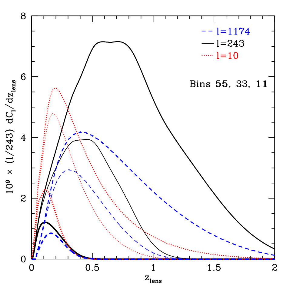
Since the shear power spectrum is an integral over the line of sight (Eq. 6), we can analyze the redshift dependence of the integrand, or kernel of the projected shear power. Recall that is the lens redshift. In particular, we expect that for small redshifts the contribution goes to zero since gets small and for a fixed multipole the scales probed get small and the mass power leading to shear decreases. (Alternately, if one considers constant fractional distance intervals , then the path length itself gets small.) For high lens redshifts, the lens-source distance gets small and again the integrand vanishes. Thus the kernel support peaks at intermediate lens redshifts, although the peak does shift to higher redshifts as the source distribution, i.e. , does. (Note that the rule of thumb that lensing is strongest at a conformal distance midway between the source and observer is more directly relevant to the lensing cross-section than to the shear power contribution.)
Figure 4 illustrates the redshift dependence of the shear power integrand for several values of multipole and source redshift bin. We show small, medium, and large and the autopower in bins 1 (), 3 (), and 5 (). Note that the peak for (1.25, 2.8) is at (0.4, 0.7). There is a long tail though to higher lens redshifts. Turned around, one could say that to probe gravitational lensing in the universe out to requires sources out to .
For cosmological constraints, what is of greater importance than where the shear power peaks is where lies the innate information about the cosmological parameters. That is, does information on different cosmologies exhibit a similar redshift weighting as the overall shear power integrand, or does higher redshift data, for example, show greater cosmological leverage? Figure 5 examines this issue with respect to the dark energy equation of state parameters and .


Considering the finite difference between the kernel supports for cosmologies with two different parameter values (all other parameters held fixed), e.g. effectively , the contributions are seen to be essentially comparable regarding the peak redshift to the shear power itself. For , there is a slight shift in leverage to higher peak redshifts, e.g. the peak for , bin 3 is rather than 0.45. The persistence of dark energy to higher redshifts through a positive increases the cosmology signal at high redshift, while a more negative diminishes the high redshift dark energy density and decreases the signal at high redshift. In both cases, however, the rise from small is pushed to larger than in the power kernel. This makes sense since low redshift cosmology is insensitive to the value of and even more so , and so the leverage is delayed.
We examine the impact of the survey redshift depth on the dark energy equation of state figure of merit in Sec. IV.5, where we also investigate the interaction with fiducial cosmology.
IV.4 Source Density and Sky Area
Another important aspect of survey design concerns the number density of source galaxies. The large number density of galaxies useful for shear measurements that become available with a small point spread function is one of the major advantages of space-based observations [19]. The density involves several factors, including the PSF characterization and the redshift depth (since the number density is projected along the line of sight, plus the galaxy size distribution varies with redshift).
Figure 6 shows that greater source density has a strong effect on figure of merit, with almost a linear dependence in the range of of interest (the improvement does flatten out at higher values, as the shape noise term becomes negligible). This study treats as an isolated parameter, and does not account for the accompanying gain in PSF characterization likely to come from a higher density of sources and star calibrations; it also holds the survey depth fixed. The fitting function over the range plotted is given by
| (27) |

The total number of lensed sources also scales with the sky area, or fraction . More sources implies more information and so the figure of merit increases with sky area. The systematics associated with weak lensing, in photometric redshifts and in shear measurements, are not taken to provide a systematic floor traditionally, i.e. the shear power spectrum uncertainty has a factor outside all the error contributions and so continues to drop with ever greater area. Whether this is realistic or not is an open question. However, priors that are placed on marginalized parameters accounting for these systematics do break the linear scaling.
We examine the dependence of the dark energy parameter estimation and figure of merit on the sky area for the particular case of a prior on the photometric redshift bias of . This should be a fairly generic representative of the behavior among the systematics. For relatively small survey area, the statistical leverage of the survey data itself provides the limit on cosmological parameter estimation, from fitting for all the systematics, and the redshift bias prior is not so important. With large sky area, however, the other contributions are well enough determined that they become of the same order as the prior on and so the prior plays an important role. See, for example, Fig. 7 of [11]. The result is that the cosmological parameter estimation (FOM) slows down in its improvement with , although it does not reach a ceiling.
Figure 7 illustrates the change in scaling. Note that even for a survey area of 1000 deg2 the improvement goes more slowly than linearly with . In the cosmological parameter determination there is a noticeable bend in the scaling between 4000 and 10000 deg2, after which the slope is shallower. A fitting function is
| (28) |
where sky area is in units of square degrees.

IV.5 Effect of Fiducial Model
One aspect we do not have control over in the survey design is the true cosmological model. In the projections for how well a survey will constrain the cosmological parameters, the true values of the parameters can have an impact. Here we examine not only the extent of the influence on the parameter estimation but whether one would be led to optimize survey design differently depending on what one believed the true cosmology was.
In general, one expects that as the dark energy persists to higher redshift, e.g. if its equation of state is closer to zero, its effects should be more visible in the shear power spectrum and it should be better constrained. Figure 8 shows that this is indeed the case. For a shift from to less negative values, the area figure of merit in the dark energy equation of state - plane increases by
| (29) |
That is, a shift boosts the FOM by a factor 1.6.

Note that here denotes the effective constant dark energy equation of state, defined for the dynamical equation of state case using the rule of thumb that the effective value . We have verified that this holds true, e.g. the results for , agree with to better than 4%, and likewise for , and . For fiducial models with more negative than , the change in FOM has less strong dependence since there is little contribution from the higher redshift bins regardless of the exact value of . The scatter in the figure curves near is a numerical artifact from interaction of the small step size (so as not to cross ) with the dark energy perturbation evolution.
These results show that weak lensing surveys may have more probative power than expected from taking a CDM fiducial cosmology. However, we have no control over what the true cosmology is, so what we do need to check is how sensitive conclusions about survey design are to the fiducial model. We would not necessarily want to choose survey requirements that are near optimal for one cosmology but inefficient for another. Figure 9 demonstrates that the survey requirements, with regards to the survey depth at least, are robust with respect to fiducial cosmology.

The first important result is that the survey depth is a crucial factor in the cosmological power of the survey. A survey whose median source depth is has a 40% improvement in FOM over one with , all else held fixed. However, going deeper than does not lead to any continued substantial gain. Thus, is near optimal for survey design. The second important point is that this optimum is not sensitive to the (uncontrollable) true cosmology. Models with effective dark energy equations of state between and all follow this rule, with the FOM as a function of (normalized to the case) differing by less than 3% between them. An excellent fit for the FOM as a function of survey depth over the range plotted is
| (30) |
V Conclusions
Weak gravitational lensing can be a powerful probe into the cosmological model, testing both the expansion history and growth of large scale structure. This sensitivity also requires that a broad array of physics be included when calculating the weak lensing shear power spectrum and its constraints on cosmological parameters. We include the effects of dynamical dark energy, spatial curvature, neutrino masses, and gravitational modifications into a weak lensing Fisher code, together with systematics from photometric redshift measurements, shear measurements, and nonlinearities in the mass power spectrum.
This flexibility allows us to carry out studies analyzing the effects of each element of an expanded parameter space, of systematic uncertainties, and of survey characteristics on the ability for weak lensing to probe cosmology. We show that allowing growth of structure some independence from the expansion history, through the gravitational growth index , i.e. relaxing the dictum of general relativity, enlarges the dark energy equation of state - contour area by a factor 2, but could lead the detection of new aspects of gravity. We find that including a systematic uncertainty in the nonlinear regime behavior of the matter power spectrum has little effect – if the dependence of the modification is known; ignoring the uncertainty (or getting the dependence wrong) can lead to substantial bias in cosmology.
Systematics control in photometric redshifts and shear measurement are, as is well known, critical. The cumulative effect of these uncertainties is especially powerful. The systematics feed strongly into the survey design, for example an improvement in shear measurement allowing a higher effective number of galaxies yields a substantial improvement in the dark energy figure of merit.
We have presented a number of illustrative survey characteristic analyses, giving accurate fitting formulas for the effect on the dark energy figure of merit with source density, survey depth, and sky area. An interesting point is that the fiducial cosmology can have a substantial impact on the figure of merit, but fortunately the behavior with survey characteristics (at least as far as depth) is nearly independent of fiducial model. Thus survey design can focus on systematics, within the control of experimental, simulation, and theory efforts. Given these efforts, weak lensing promises a cornucopia of knowledge about cosmology, gravity, and fundamental physics.
Acknowledgements.
We thank Dragan Huterer for useful discussions. This work has been supported in part by the Director, Office of Science, Office of High Energy Physics, of the U.S. Department of Energy under Contract No. DE-AC02-05CH11231, and also by the World Class University grant R32-2008-000-10130-0 through the National Research Foundation, Ministry of Education, Science and Technology of Korea (EL,RN). RN acknowledges partial support by NASA LTSA Carlo 23235-24523-44.References
- [1] D. Munshi, P. Valageas, L. van Waerbeke, and A. Heavens, Phys. Rep. 462, 67 (2008), eprint arXiv:astro-ph/0612667.
- [2] D. Huterer, General Relativity and Gravitation 42, 2177 (2010), eprint arXiv:1001.1758.
- [3] M. Bartelmann and P. Schneider, Phys. Rep. 340, 291 (2001), eprint arXiv:astro-ph/9912508.
- [4] H. Hoekstra and B. Jain, Annual Review of Nuclear and Particle Science 58, 99 (2008), eprint arXiv:0805.0139.
- [5] S. F. Daniel and E. V. Linder, Phys. Rev. D 82, arXiv:103523 (2010), eprint 1008.0397.
- [6] V. Acquaviva, C. Baccigalupi, and F. Perrotta, Phys. Rev. D 70, 023515 (2004), eprint arXiv:astro-ph/0403654.
- [7] C. C. Dyer and R. C. Roeder, ApJ 180, L31 (1973).
- [8] E. V. Linder, J. Cosmology Astropart. Phys 3, 19 (2008), eprint arXiv:0711.0743.
- [9] A. Lewis, A. Challinor, and A. Lasenby, ApJ 538, 473 (2000), eprint arXiv:astro-ph/9911177, URL http://camb.info/.
- [10] G. M. Bernstein, ApJ 695, 652 (2009), eprint arXiv:0808.3400.
- [11] Z. Ma, W. Hu, and D. Huterer, ApJ 636, 21 (2006), eprint arXiv:astro-ph/0506614.
- [12] D. Huterer, M. Takada, G. Bernstein, and B. Jain, MNRAS 366, 101 (2006), eprint arXiv:astro-ph/0506030.
- [13] R. E. Smith, J. A. Peacock, A. Jenkins, S. D. M. White, C. S. Frenk, F. R. Pearce, P. A. Thomas, G. Efstathiou, and H. M. P. Couchman, MNRAS 341, 1311 (2003), eprint arXiv:astro-ph/0207664.
- [14] D. Huterer and M. Takada, Astroparticle Physics 23, 369 (2005), eprint arXiv:astro-ph/0412142.
- [15] H. Oyaizu, M. Lima, and W. Hu, Phys. Rev. D 78, 123524 (2008), eprint arXiv:0807.2462.
- [16] D. Huterer and E. V. Linder, Phys. Rev. D 75, 023519 (2007), eprint arXiv:astro-ph/0608681.
- [17] E. V. Linder, Phil. Trans. Roy. Soc. A (2011), eprint arXiv:1103.xxxx.
- [18] A. Stril, R. N. Cahn, and E. V. Linder, MNRAS 404, 239 (2010), eprint arXiv:0910.1833.
- [19] M. M. Kasliwal, R. Massey, R. S. Ellis, S. Miyazaki, and J. Rhodes, ApJ 684, 34 (2008), eprint arXiv:0710.3588.