Fluctuations and phase transitions in Larkin-Ovchinnikov liquid crystal states of population-imbalanced resonant Fermi gas
Abstract
Motivated by a realization of imbalanced Feshbach-resonant atomic Fermi gases, we formulate a low-energy theory of the Fulde-Ferrell and the Larkin-Ovchinnikov (LO) states and use it to analyze fluctuations, stability, and phase transitions in these enigmatic finite momentum-paired superfluids. Focusing on the unidirectional LO pair-density wave state, that spontaneously breaks the continuous rotational and translational symmetries, we show that it is characterized by two Goldstone modes, corresponding to a superfluid phase and a smectic phonon. Because of the liquid-crystalline “softness” of the latter, at finite temperature the 3d state is characterized by a vanishing LO order parameter, quasi-Bragg peaks in the structure and momentum distribution functions, and a “charge”-4, paired Cooper-pairs, off-diagonal-long-range order, with a superfluid-stiffness anisotropy that diverges near a transition into a nonsuperfluid state. In addition to conventional integer vortices and dislocations the LO superfluid smectic exhibits composite half-integer vortex-dislocation defects. A proliferation of defects leads to a rich variety of descendant states, such as the “charge”-4 superfluid and Fermi-liquid nematics and topologically ordered nonsuperfluid states, that generically intervene between the LO state and the conventional superfluid and the polarized Fermi-liquid at low and high imbalance, respectively. The fermionic sector of the LO gapless superconductor is also quite unique, exhibiting a Fermi surface of Bogoliubov quasiparticles associated with the Andreev band of states, localized on the array of the LO domain-walls.
I Introduction
I.1 Background
I.1.1 Imbalanced resonant atomic gases
Experimental progress in trapping, cooling and coherently manipulating Feshbach-resonant atomic gases opened an unprecedented opportunity to study degenerate strongly interacting quantum many-body systems in a broad range of previously unexplored regimes [1, 2, 3, 4, 5, 6]. These include paired fermionic superfluids (SF) (with -wave SF now readily realized [7, 8, 9, 10, 11], and -wave SF under extensive current study[12, 13, 14, 15, 16, 3]), the associated Bardeen-Cooper-Schrieffer (BCS) to Bose-Einstein condensation (BEC) crossover[17, 18, 19, 20, 21, 22, 23, 24, 25, 3], Bose-Fermi mixtures[26], bosonic molecular superfluids[27, 28, 29, 30], and many other states and regimes[31] under both equilibrium and nonequilibrium conditions[32, 24, 33]. In addition to the tunability of the Feshbach-resonant interaction strength (and its effective sign), temperature, and many types of external perturbations, a species number imbalance in e.g., a two atomic hyperfine-states mixture turned out to be an extremely fruitful experimental knob[34, 35, 36, 37].
A nonzero species imbalance frustrates conventional BCS pairing of a two-species Fermi gas[38, 39, 40, 41] and the associated BCS-BEC crossover[42, 43, 44, 45, 46], driving quantum phase transitions out of a paired superfluid to a variety of interesting possible ground states and thermodynamic phases[48, 49, 44, 47, 46, 50, 51]. This rekindled considerable theoretical activity in the context of species-imbalanced resonant Fermi gases[52, 53, 54, 55, 56, 57, 58, 59, 60, 61, 62, 63, 64, 65, 66, 67, 4, 68, 69, 70, 71, 72]. The identification of the number species imbalance with the magnetization of an electronic system, and the chemical potential difference with an effective Zeeman energy, connects these recent atomic gases studies with a large body of research on solid state electronic superconductors under a Zeeman field[73, 75, 76, 77], as well as extensively studied realizations in nuclear and particle physics[78, 79, 80, 81]. The obvious advantage of the current atomic system is the aforementioned tunability, disorder-free “samples”, and absence of the orbital part of the magnetic field, that always accompanies a solid-state charged superconductor in a magnetic field[82]. In these neutral paired superfluids the orbital field effects can be independently controlled by a rotation of the atomic cloud[83].
As illustrated in Fig.1, among many interesting features, such as the gapless imbalanced superfluid ()[44, 47, 45, 46], ubiquitous phase separation[40, 44, 47, 4], tricritical point[69, 72], etc., observed experimentally[34, 35, 36, 37] and studied extensively theoretically[4, 6], the interaction–imbalance BEC-BCS phase diagram is also predicted[52, 44, 4, 46, 70, 71] to exhibit the enigmatic Fulde-Ferrell-Larkin-Ovchinnikov state (FFLO)[76, 77]. First predicted in the context of solid-state superconductors over 45 years ago[76, 77], the FFLO states has so far eluded a definitive observation, though some promising solid state[84] and quasi-1d atomic[85] candidate systems have recently been realized.
At its most generic level the FFLO state[86] is a fermionic superfluid, paired at a finite center of mass momentum. Generically such a state spontaneously “breaks” gauge and translational symmetry, i.e., it is a periodically-paired superfluid (superconductor), akin to a supersolid[87, 88, 89, 90], and thus can appropriately be called a pair-density wave (PDW)[91, 92]. Microscopically, it is driven by Fermi surface mismatch[76, 77] due to an imposed pairing species number (and/or mass[93]) imbalance. As a compromise between the superfluid pairing and an imposed imbalance, at intermediate values of the latter, the superconducting order parameter condenses at a set of finite center-of-mass momenta determined by the details of the Fermi surface mismatch and interactions, thereby self-consistently leading to FFLO pairing between these imbalanced fermionic species. At sufficiently large imbalance, or equivalently at the upper-critical Zeeman field (corresponding to the chemical potential difference of the two pairing species) no compromise is possible, and instead a transition to the normal state takes place.
I.1.2 Mean-field energetic stability of FFLO states
The original predictions by Fulde and Ferrell (FF), and by Larkin and Ovchinnikov (LO) were followed by extensive studies of the FFLO states[78, 79, 80, 81], though exclusively confined to their energetics in the BCS limit. Stimulated by the aforementioned potential realization in imbalanced resonant Fermi gases, the recent revival of the subject extended the analysis to the full range of the BCS-BEC crossover[52, 44, 4, 69, 70, 94]. As illustrated in Fig.1, the key observation is that, despite of strong interactions, within a single BdG treatment the conventional FFLO state (those originally proposed by FF and LO) remains quite fragile, confined to a narrow sliver of polarization in the BCS regime[44, 4].
However, motivated by earlier studies of the Bogoliubov-de Gennes (BdG) equation[95, 96, 97], combined with finding of a negative domain-wall energy in an otherwise fully-paired singlet BCS superfluid in Zeeman field[97, 98], recent studies have quite convincingly argued, that a more generic pair-density wave state (that includes a larger set of collinear wavevectors) may be significantly more stable. Analogously to a strongly type-II superconductor, that undergoes a continuous transition into a vortex state at a lower-critical orbital field [99, 100, 101] (that is significantly below the thermodynamic field, ) in the current system, a Zeeman-field (the chemical potential imbalance) can drive a nucleation of domain-walls in the superfluid order parameter above the lower-critical Zeeman field that is below the bulk mean-field value . Thereby, the excess of the majority fermionic atoms (polarization) in an imbalanced system can be continuously accommodated by the sub-gap states localized on the self-consistently induced domain-walls, through a continuous commensurate-incommensurate (CI) Pokrovsky-Talapov (PT) type of transition[102] from a fully paired s-wave superfluid to a Larkin-Ovchinnikov like periodic state of domain walls[103, 104]. This picture, illustrated in Fig.2 resembles the soliton mechanism for doping of polyacetylene[105]. The domain-wall description, that is explicitly realized in one-dimension (1d) through exact BdG[95] and Bethe ansatz[106, 107] solutions and via bosonization[108, 109], is complementary, but not qualitatively distinct from the more familiar single cosine form of the LO state[77].

The latter, “soft” pair-density wave is a more appropriate description near the transition into the normal state, where the pair-order parameter is naturally small, and a Landau expansion in the leading harmonic, is expected to be valid. On the other hand, clearly, far below (e.g., near transition from the fully-paired uniform singlet BCS state) the periodic soliton state is a quantitatively better description as it more accurately captures the strong pairing at , confining the “normal” regions that accommodate the imposed fermion imbalance to the narrow gapless domain-walls between . Upon increasing above the density of domain-walls grows, eventually overlapping at , thereby interpolating between the two limiting descriptions of the LO state. This picture is explicitly realized in the exact 1d solutions[95, 106, 107, 108] and emerges from the numerical BdG studies[96, 97]. Furthermore, the lack of a single nesting for , to which the fragility of the LO state is usually attributed is irrelevant when the LO order parameter exhibits a broad spectrum of (set by ), as in its soliton form above .
The LO state can be equivalently thought of as a periodically ordered micro-phase separation between the normal and paired states, that naturally replaces the macro-phase separation[81, 40] ubiquitously found in the BCS-BEC detuning-imbalance phase diagram[44, 47, 4].
It is clear that the standard (even multi-wavevector) Landau treatments valid near and analytical BdG analysis of a single FF plane-wave state (exhibiting no amplitude nodes)[4] fail to capture above quantitatively important ingredients. These treatments are therefore not necessarily quantitatively trustworthy in their prediction of the energetic range of stability (location of ) of the LO state (they are however reliable for the prediction of ), and in our view need to be reexamined.
I.1.3 Fluctuation in the FFLO states
The microscopic question of the energetic stability of FFLO states is certainly an extremely important one and has dominated most of the research on the subject to date. However, given the extensive 45-year history of the topic, it is astounding that the equally basic complementary question of the nature of Goldstone modes description and their fluctuations within the FFLO states received so little attention,[110, 111] until our study of the problem, reported in a recent Letter[112]. From the general symmetry principles the FFLO states’ low-energy phenomenology is expected to be significantly richer than that of a homogeneous fully gapped superconductor, whose low-energy phenomenological (Ginzburg-Landau and xy-model) description long predated the microscopic theory by BCS[99, 100, 101]. Namely, in addition to a local superfluid phase degree of freedom, the low-energy modes include the phonons (a single scalar one in the case of a uniaxial LO state) of the periodic superconducting structure, as well as gapless polarized (single-species) fermionic atoms confined to a fluctuating periodic array of two-dimensional domain walls[112, 111].
In the isotropic realization (e.g., in cold atoms in an isotropic trap) of interest to us, the FFLO states spontaneously break a continuous rotational (in addition the translational) symmetry akin to smectic liquid crystals, in contrast to their solid state density-wave analogs. Consequently, as was originally anticipated by Shimahara[110], and was demonstrated in our recent work[112], to be explored in greater detail below, their Goldstone modes are qualitatively “softer”, and therefore exhibit far stronger fluctuations. These can either completely destabilize the (otherwise energetically stable) FFLO state, or can qualitatively modify its mean-field form and properties. This general picture therefore reveals that the complexity of the FFLO state beyond its mean-field cartoon requires the understanding of subtle interplay of superfluidity, liquid-crystallization, and anisotropic Fermi surface physics.
With the above motivation in mind, in a recent Letter[112] above questions were formulated and carefully explored. Namely, as illustrated in a schematic phase diagram in Fig.3, supported by the aforementioned studies[95, 96] and the exact 1d solutions[95, 108, 109], we assumed that a striped (unidirectional) FFLO state (that we refer to as LO), characterized by a collinear set of wavevectors is energetically (microscopically) stable over an experimentally accessible portion of the detuning-imbalance phase diagram. We then formulated the model for the low-energy Goldstone modes fluctuations and fermionic excitations in the LO state and used it to study the stability of the state to quantum and thermal fluctuations, as well as explored the fluctuation-driven phenomenology, topological defects, novel quantum liquid crystal phases, and the associated phase transitions[112]. In the present manuscript we present a significantly more extensive description of these findings and the details of the associated calculations.
I.1.4 Relation to other systems and studies
Although physically quite distinct, some of our motivation and findings[112] are closely related to studies in solid state realizations, such as the putative FFLO states in heavy-fermion (CeCoIn5) and organic (-(BEDT-TTF)2Cu(NCS)2) superconductors[113, 114], the striped (and spiral) states in high-Tc superconductors and nickelates and more generally strongly correlated doped Mott insulators[115, 116, 117, 118, 119, 120], spiral states in helimagnets[121, 122, 123], partially-filled high Landau level 2d electron gas[124, 125, 126], charge-density waves in anisotropic metals[127], and others. Among a number of physical properties special to resonant atomic Fermi gases, one key qualitatively distinguishing feature in our study is that the FF and LO states spontaneously breaks continuous translational and orientational symmetries of an isotropically trapped Fermi gas. As first emphasized in Refs.110, 112 this latter property is responsible for the qualitatively enhanced fluctuations, that lead to the predicted universal power-law correlations (5),(7) persisting throughout the 3d quasi-long-range ordered FFLO phase, rather than just at a critical point. Thus, such FF and LO states (and its descendents) are qualitatively distinct from their mean-field form[76, 77], akin to a distinction between, e.g., a 2d xy model and a long-range ordered 3d ferromagnet. In contrast, the aforementioned states in the solid state systems, by their very definition only break discrete point-group crystal symmetries, and therefore exhibit quite tame Gaussian fluctuations inside the phase, with these periodic states only quantitatively distinct from their mean-field form.
I.1.5 Outline
The rest of the paper is organized as follows. We conclude the Introduction with the summary of our main results. Then, in Sec.II we use a microscopic description of the imbalanced resonant atomic Fermi gas to derive in the weakly-interacting BCS limit the corresponding Landau theory (along with microscopic expressions for its parameters) valid near transition to the normal state. In Sec.III we discuss symmetries of two generic class of FFLO states, construct corresponding order parameters and derive from the Landau theory the corresponding models for their Goldstone modes. As we argue, these models provide universal descriptions of low-energy fluctuations in the FF and LO class of states, beyond the limit of validity of their microscopic BCS-limit derivation. In Sec.IV we complement this derivation (valid near ) by an analysis of an array of fluctuating domain walls, valid near . In Sec.V we use these low-energy universal models to analyze quantum and thermal fluctuations in the FF and LO class of states, paying particular attention to elastic nonlinearities that (as we show) are qualitatively important at a finite temperature. Then in Sec.VI we classify and discuss energetics of topological defects in the LO state. In Sec.VII we use this information to uncover a variety of exotic “daughter” liquid-crystal phases that emerge as a result of unbinding different combinations of topological defects, and discussion corresponding phase transitions. In Sec.VIII we extend the model to include the coupling of the Goldstone modes to gapless fermionic atoms, and comment on their effects. In Sec.IX we use local density approximation (LDA) to put our results in the context of trapped atomic gases and discuss experimental probes of our predictions. We conclude in Secs.X,XI,XII with discussions of experimental probes, open questions and a summary of our study. In appendices A and B we provide technical details for the microscopic derivation of the Ginzburg-Landau expansion near and finite-size scaling analysis of smectic fluctuations, respectively.
I.2 Results
Before turning to the derivation and analysis of the model, we summarize the key predictions of our work, previously reported in Ref.112. Because our predictions[128] are based on general symmetry principles, supported by detailed microscopic weak-coupling calculations, they are generic and robust to variation in microscopic details. At a very general level, we demonstrate that (in contrast to the conventional uniform superfluid and FF states) a unidirectional (striped) LO superfluid exhibits two Goldstone modes, and . These correspond to two coupled smectics phonons, or equivalently the superfluid phase and a nonlinearly-coupled smectic phonon mode , with the wavevector characterizing the LO state.
Through robust symmetry arguments, complemented by an explicit microscopic derivation (valid in the BCS regime, near the LO to normal state transition at ), we show that the low-energy universal (classical) LO Hamiltonian governing fluctuations of these Goldstone modes is given by
This Hamiltonian form, familiar from studies of conventional smectic liquid crystals, encodes the underlying rotational invariance through the vanishing of the modulus and the specific form of the nonlinear elastic terms in [129, 130, 131, 132]. In above refer to axes that are parallel and perpendicular to the LO ordering wavevector , respectively. In the weak-coupling BCS limit, we derive explicit expressions for the above Goldstone-modes moduli, , , (), given by
| (2a) | |||||
| (2b) | |||||
| (2c) | |||||
also given in Eqs.(80),(81) of the main text. Among these predictions, we find that the LO state is a highly anisotropic superfluid, with the ratio of superfluid stiffnesses given by
| (3) |
vanishing on the approach to the upper-critical Zeeman field , that marks the mean-field transition to the normal state at which the LO order parameter vanishes. is the zero-field BCS order parameter.
We find the FF state to be even more exotic. In contrast to other homogeneous superfluids (described by an xy-model), its single superfluid Goldstone mode is described by above smectic Hamiltonian, with an identically vanishing transverse superfluid stiffness, , a reflection of the rotational invariance of the spontaneous current to an energy-equivalent ground state. Thus we show that a resonant imbalanced Fermi gas, confined to an isotropic trap gives a natural realization of a quantum (superfluid) smectic liquid crystal.
As a consequence of the spontaneous breaking of continuous spatial symmetries (contrasting with its solid state realizations, where only discrete point-group (lattice) symmetries are spontaneously broken)[113, 115, 118, 119, 120, 121, 123, 124, 125] the Goldstone mode excitations in the FF and LO states are of qualitatively lower energy. As a result, the fluctuations in such superfluid smectic states are qualitatively stronger. Specifically, we find that while they are stable to quantum fluctuations, in 3d the LO and FF long-range orders are marginally unstable at any nonzero , with the LO order parameter (with Dirichlet boundary conditions; for a more general case, see Sec.X of the main text)
| (4) | |||||
vanishing in the thermodynamic limit (a large cloud with atom number and cloud size ), suppressed to zero by thermal phonon fluctuations, and is therefore strictly speaking homogeneous on long scales. The resulting superfluid state is thus an “algebraic topological” phase with no long-ranged translational order. Namely, beyond mean-field theory it is instead characterized by power-law order-parameter correlations, distinguished from the spatially short-ranged disordered phase by confined topological defects (bound dislocations), not by a nonzero LO order parameter. It is therefore a 3d analog of the more familiar quasi-long-range ordered superfluid film and a 2d easy-plane ferromagnet.
There are a number of interesting consequences of this finding. For example, as illustrated in Fig.21, we predict that in 3d[133] the static structure function in the LO state exhibits universal anisotropic quasi-Bragg peaks (akin to a conventional smectic liquid crystal[134, 135]), with -th order peak given by
| (5) |
rather than the true -function Bragg peaks of e.g., a long-range-ordered pair-density wave in a crystalline environment. In above the anomalous Caillé exponent[134] is given by
| (6) |
We similarly find that the momentum distribution function of pairs displays a power-law form around the reciprocal lattice momenta set by of ,
| (7) |
as illustrated in Fig.(20). This power-law is a reflection of a striking pair-condensate depletion to zero by the divergent finite LO Goldstone-mode fluctuations even in 3d, akin to the Landau-Peierls[136, 137] behavior of films of a conventional superfluid and 2d crystals[138, 139, 140, 141]. Such static correlations in the LO state can be computed asymptotically exactly, as was first done for a conventional smectic liquid crystal[134, 131, 132]. This fluctuation-driven 3d power-law phenomenology is a unique feature of a unidirectional (collinear wavevectors) FFLO state. It is not exhibited by crystalline FFLO phases with multiple non-collinear ordering wavevectors[79, 78], that, in contrast are characterized by the long-range positional order and a nonzero pair-condensate, that is stable to thermal fluctuations.
As with treatments of the LO state, where long-range order is assumed[113, 118], in this algebraic LO phase we also find an unusual topological excitation – a half vortex bound to a half dislocation – in addition to integer vortices and dislocations. These are illustrated in Figs.8,9, and 10.
In 2d, at nonzero the LO state is even more strongly disordered, at intermediate scales characterized by universal power-law phonon correlations and concomitant short-range positional order with Lorentzian structure function peaks, controlled by a nontrivial exactly calculable fixed point[132]. Asymptotically, however, at arbitrary low temperature the 2d LO state is unstable to proliferation of dislocations[142]. The state that results from such dislocated superfluid smectic is either a “charge”-4 (paired Cooper pairs)[143] nematic superfluid[112, 119] or a nematic (possibly “fractionalized”b) Fermi liquid[117, 126], latter qualitatively the same as the deformed Fermi surface state [49].
More generally, while analyzing defects-driven continuous transitions out of the LO state, we uncover a rich array of descendent states, that generically must intervene between the LO superfluid and a fully-paired conventional (isotropic and homogeneous) superfluid and a conventional Fermi liquid. If indeed the 3d LO state is energetically stable, as argued above, we expect these novel states to appear in the region collectively denoted “LO liquid crystals” of the detuning-polarization phase diagram of Fig.3. They include a nonsuperfluid smectic (, driven by an unbinding of integer -vortices), and a superfluid (, driven by a proliferation of integer -dislocations) and a nonsuperfluid (, driven by an unbinding of both vortices and dislocations) nematics, and the corresponding isotropic states, when disclinations also condense. In addition, we predict a variety of topologically-ordered isotropic and nematic “fractionalized” Fermi-liquid states (, , , and others), that are distinguished from their more conventional fully-disordered forms by gapped (bound) half-integer defects. These phases are summarized by a schematic phase diagram illustrated in Fig.4. We now turn to the derivation of these predictions.
II BCS theory of imbalanced resonant Fermi gas
II.1 Model
We begin with the one-channel model of two-species, resonantly interacting Fermi gas, appropriate for the experimentally relevant broad Feshbach resonance[4, 5, 6]. In the grand-canonical ensemble, it is described by a Hamiltonian
| (8) |
with the two atomic species (labeling the hyperfine states ) open-channel fermions created by the anticommuting operator
| (9) |
with the single-particle energy , mass , and system’s volume (henceforth set to ).
In above we introduced two distinct chemical potentials, to impose numbers of two separately conserved atomic species, , or equivalently the total fermion number and the atom species imbalance . Equivalently, the two species chemical potentials and are related to the total-number chemical potential and the species-imbalance chemical potential , latter corresponding to the pseudo Zeeman energy. The imbalanced resonant Fermi gas thermodynamics as a function of , i.e., the extension of the BEC-BCS crossover to a finite imbalance can be computed by a variety of theoretical techniques, including quantum Monte Carlo [42], mean-field theory [44, 47, 45, 4, 69], the large- (fermion flavor) [144, 145] and -expansions [146].
The attractive interaction is parameterized by a short-range s-wave pseudopotential with a strength . Through a standard T-matrix scattering calculation[147, 148], that gives the two-atom s-wave scattering amplitude, , the pseudo-potential parameter can be related to the experimentally determined, magnetic field dependent [149] scattering length
| (10) |
where the ultraviolet-divergent second term is regularized by a microscopic momentum cutoff scale set by the range of the potential, . This gives (with hereafter)
| (11a) | |||||
| (11b) | |||||
where is the effective screened coupling and is the critical coupling (set by the zero-point energy at scale ) at which a molecular bound state appears and the scattering length diverges. The above relation allows a definition of the model and therefore a reexpression of physical observables in terms of the experimentally defined (UV-cutoff independent) scattering length .
To treat the many-body problem, (8), we utilize the standard mean-field analysis[44, 4] (quantitatively valid deep in the BCS regime, , but expected to be qualitatively valid throughout) by first assuming an expectation value
| (12) | |||||
corresponding to pair condensation at a superposition of finite momenta , with the set of and to be self-consistently determined. With this mean-field assumption, , in Eq. (8), reduces to the standard BCS mean-field form:
| (13) | |||||
that can equivalently be obtained using a Hubbard-Stratonovich transformation and a saddle-point approximation on the coherent state path-integral formulation of the problem.
Although the resulting mean-field Hamiltonian is quadratic in the fermionic operators, its diagonalization for a generic (an arbitrary set of Fourier components ) is only possible through a numerical self-consistent solution of the Bogoliubov–de Gennes equations[95, 96].
Analytical progress is however possible through two complementary approaches. One is to specialize to a single Fourier component, FF state[76], that is self-consistently determined through the -dependent gap equation, (12), equivalent to the ground-state energy minimization. This approach allows for a computation of the ground-state energy that is fully nonlinear in . However, as emphasized in the Introduction with regard to learning about a more generic amplitude-modulated FFLO state this simplifying specialization to a single Fourier component is only harmless near the normal-to-FFLO state transition at the mean-field upper-critical field , where is small and physics is well-approximated by the lowest dominant harmonic.
II.2 Bogoliubov–de Gennes analysis of the Fulde-Ferrell state
II.2.1 Ground state solution
Specializing to the Fulde-Ferrell (single harmonic, ) state simplifies the mean-field Hamiltonian, (8), allowing for a straightforward diagonalization[76, 44, 4] of the the associated Bogoliubov–de Gennes equations. A standard analysis[4] gives the (fermionic) Bogoliubov quasi-particle operators,
| (14a) | |||||
| (14b) | |||||
with the orthonormal coherence factors [99, 100, 101]
| (15a) | |||||
| (15b) | |||||
ensuring the canonical anticommutation relations, . In terms of these quasi-particles, the Hamiltonian reduces to a diagonal quadratic form
| (16) | |||||
with the ground state energy given by
| (17) | |||||
In above, we defined the excitation energy for spin state
| (18a) | |||||
| (18b) | |||||
with
| (19a) | |||||
| (19b) | |||||
and , the average and difference chemical potentials, respectively. The introduction of -functions in above expressions divides the momentum space into three regions, for given by: (1) such that and , (2) such that and (3) such that , (it is easy to see that the cannot both be negative), and by construction ensures a positive-definite excitation spectrum above the FF ground state
| (20a) | |||||
| (20b) | |||||
with the atom vacuum. The first form demonstrates that the FF ground state can be formally thought of as the Fermi sea of negative energy Bogoliubov “quasi-particles” added to the BCS state (that is not the ground state) with the center of mass momentum . The second form, above, shows that equivalently the FF ground state corresponds to a finite center of mass momentum () BCS state with unpaired atoms from the two momenta sets and , defined above.
This analysis thus suggests a possibility of two distinct FF states, FFfs1 and FFfs2, that exhibit a single- and two-species Fermi surfaces, respectively, with their volume difference set by the imposed species imbalance[62].
II.2.2 Analysis near
The energetic stability of the state is controlled by , that deep in the BCS limit was first computed by Fulde and Ferrell[76]. Its full behavior throughout the BCS-BEC crossover generally requires a combination of numerical and analytical analysis. This led to the prediction of a narrow sliver of stability of the FF state confined to the BCS side of the crossover, [44, 4]. However, as discussed in the Introduction, given the expected unfavorable nature of the FF state (lacking the amplitude nodes necessary to accommodate the imbalanced atoms) this analysis is unlikely to shed light on the stability of other (e.g., LO type) states far below the transition to them. Nevertheless, because the transition at the upper-critical field (at least in mean-field theory) is expected to be continuous and therefore small, growing from , can be analyzed analytically by Taylor-expanding it in .
Taking advantage of the extensive analysis in[44, 4], near we obtain
| (21) |
where
and
| (23) |
that agree with the Larkin-Ovchinnikov result[77] obtained via a direct Landau expansion in . In above we used (10) to eliminate the interaction coupling in favor of the scattering length and then reexpressed the latter in terms of the BCS superfluid gap according to , with 3d density of states . Near its minimum can be approximated quadratically in
| (24) |
with
| (25a) | |||||
| (25b) | |||||
| (25c) | |||||
In above, is a solution of equation arising from the minimization of the ground-state energy with respect to center of mass momentum [44, 4]
| (26a) | |||||
| (26b) | |||||
Combining this value with the point at which vanishes, we obtain the N-FFLO upper-critical transition field[76, 77]
| (27a) | |||||
| (27b) | |||||
At this transition point we have
| (28a) | |||||
| (28b) | |||||
| (28c) | |||||
| (28d) | |||||
where the BCS coherence length is given by its standard expression .
Near the transition the FF quartic vertex, (23) also simplifies giving
| (29a) | |||||
| (29b) | |||||
| (29c) | |||||
which agrees precisely with perturbative LO result[77].
As we will see shortly, in single plane-wave FF state the transverse superfluid stiffness for a supercurrent flowing transversely vanishes identically, enforced by a Ward identity. As mentioned in the Introduction this property is a special feature of a single momentum component FF state and is guaranteed by the underlying rotational invariance of the spontaneous current to an energy-equivalent ground state. Thus, to correctly (even qualitatively) capture a more general FFLO (e.g., the LO) state requires the inclusion of the multiple momentum components, as in (12) and the analysis beyond the lowest-order LO treatment[77]. This unfortunately cannot be calculated analytically through the Bogoliubov–de Gennes analysis, although it quite successfully can numerically[95, 96] and through the Ginzburg-Landau expansion to which we now turn.
II.3 Ginzburg-Landau expansion near
The analytical treatment of the LO state near relies on the Ginzburg-Landau expansion in , that is small near the (in mean-field) continuous normal-to-FFLO transition [77, 150]. This expectation is explicitly supported by the exact 1d BdG solution[95] at high fields, where is indeed well-approximated by a single harmonic, with an amplitude that vanishes continuously near .
Based on these general arguments, near the Ginzburg-Landau expansion for the ground-state energy is expected to take a familiar form
where rotational invariance constrains to be a function of the magnitude of only, , and is a Fourier transform of .
It is straightforward to see that translational and rotational invariances and the quadratic form (in ) of the first term in guarantee that is independent of the type of the FFLO state, and is therefore identical to that of the FF state, ()[4]. This observation guarantees that all harmonics with magnitude become unstable at the same imbalance field , (27b), with the degeneracy only lifted by the quartic term in .
Following the standard prescription and guided by the seminal (lowest order) analysis of Larkin and Ovchinnikov[77], we now derive the quartic vertex function, , appearing in Eq.(). It, together with will then allow us to derive the key elastic moduli (compression modulus, bending rigidity, and superfluid stiffnesses) characterizing the Goldstone modes of the striped FFLO states. As first found in Ref.112, one key observation is that a derivation of a generic Ginzburg-Landau form and consequently of a generic Goldstone mode theory requires a calculation that is of higher order than that originally carried out by Larkin and Ovchinnikov[77]. In particular, as we will see below, the leading momentum dependence of the quartic coupling needs to be kept. It corresponds to an induced short-ranged current-current interaction, , with the supercurrent given by the standard expression
| (31) |
To derive the generic Ginzburg-Landau form, we use the imaginary time fermionic coherent-state path-integral formulation of the BCS problem, by computing the partition function,
| (32a) | |||||
| (32b) | |||||
where is the four-Fermi Hamiltonian, (8), Grassmann (anticommuting) fields, and the imaginary time action is given by
where for notational short-hand we defined a space-time coordinate and a single particle Hamiltonian operator, .
We use the Cooper-pair Hubbard-Stratonovich field to decouple the (quartic) pairing interaction and to integrate out the fermionic atoms:
| (34a) | |||||
| (34b) | |||||
where ,
| (35a) | |||||
| (35b) | |||||
and we defined the Ginzburg-Landau effective action
| (36) |
Taylor-expanding in powers of we compute in powers of . Relegating all technical details to Appendix A and focusing on the time-independent quartic order (in ) contribution, given by the connected fourth cumulant , we find
where
| (38a) | |||||
| (38b) | |||||
with the noninteracting fermionic Green’s function (in Fourier space) as usual given by
| (39a) | |||||
| (39b) | |||||
We focus on the FFLO type order parameter
| (40) |
with Fourier transform given by
| (41) |
We note that to go beyond mean-field, in above we included an additional long-scale positional dependence in the Larkin-Ovchinnikov order parameters on top of the short-scale mean-field periodic dependence at the LO wavevectors encoded in the plane-wave factor.
Substituting this form into , gives
| (42) | |||||
with (due to expected to be sharply peaked around ), allowing us to disentangle the sums and integrals, and the corresponding -function above, without double-counting momentum states.
To lowest order in , we ignore its dependence in , equivalent to the LO treatment[77], with , and thereby obtain the quartic vertex that determines which set of reciprocal momenta (satisfying the momentum conservation) minimizes the interaction energy, thereby defining the structure of the FFLO ground state. As found by LO[77], near it is the striped state of collinear ’s that is energetically favored and is well approximated by the lowest pair of harmonics, . Focusing on this energetically preferred (near ) LO state reduces the general form of in Eq. (42) to
| (43) | |||||
Taylor-expansion of in then gives , with
| (44) | |||||
where
| (45a) | |||||
| (45b) | |||||
already computed by LO in their mean-field approximation and in Ref. 4 from the expansion of the BdG ground state energy of the FF state discussed in Sec.II.2.
In computing the higher order term, that contains the essential current-current interaction discussed in the previous section, we will neglect contributions from the first set of terms in Eq.(43) ( and terms), because they lead to (positive current) and (negative current) contributions whose coefficients are enforced either by rotational invariance (which for transverse current each are of the coefficient of the term, required to keep the smectic phonon field “soft”), or for the longitudinal pieces are small, i.e., higher order, subleading corrections to the nonzero quadratic (in ) terms computed in the previous section.
To proceed we focus on the second term in Eq. (43), and Taylor expand it to second order in
| (46) | |||
taking advantage of momentum conservation to generate four equivalent terms such that the expression is explicitly real. In above we defined the current-current coupling matrix
| (47a) | |||||
| (47b) | |||||
where
| (48a) | |||||
| (48b) | |||||
| (48c) | |||||
| (48d) | |||||
are computed in Appendix A. Converting this Fourier space expression into real space gives
| (49a) | |||||
| (49b) | |||||
| (49c) | |||||
| (49d) | |||||
where we reconstructed the and transverse pieces (by rotational invariance) and defined the total supercurrent .
It is important to note already at this stage that the positivity of in Eq. (48) generates a positive transverse superfluid stiffness, and therefore a well-defined LO state. Furthermore, we note that (as we will see in Sec.III) the fact that and even are negative does not cause any stability difficulties as they lead to corrections to the longitudinal superfluid stiffness , a correction that is subdominant near . However, the opposite signs do suggest that below , grows, while decreases with decreasing chemical potential difference, . It is thus conceivable that the anisotropy ratio (starting at just below ) may actually grow above , i.e., that the superfluid anisotropy may reverses, something that would have striking experimental consequences.
Putting above derived ingredients together we finally obtain the sought-after Ginzburg-Landau Hamiltonian
| (50) |
where as just derived, deep in the BCS limit (large positive detuning, ) and near the transition to the polarized normal state the model parameters are given by
| (51a) | |||||
| (51b) | |||||
| (51c) | |||||
| (51d) | |||||
| (51e) | |||||
| (51f) | |||||
Based on the discussion following Eq. (49) we approximated the anisotropic tensor coupling , Eq. (47) by an isotropic one of strength set by the transverse part of , namely, , with the difference a subleading correction near . More generally (away from the weak-coupling BCS limit) these couplings can be taken as phenomenological parameters to be determined experimentally.
III Theory of Goldstone modes in striped FFLO states
III.1 Landau theory
The general form of the Ginzburg-Landau model (50) derived in the previous section has a much broader range of applicability, even if our derivation and microscopic predictions for the associated coupling constants in Eq. (51) only apply in the BCS regime, near . Independent of the microscopics, the key ingredient of is that it captures the imbalanced atomic Fermi system’s energetic tendency to pair at a finite momentum, and thereby forms a pair-density wave characterized by a reciprocal lattice vector with magnitude and spontaneously chosen orientation. More generally, we expect the quadratic (in ) part of
| (52) |
to be characterized by a more generic differential kernel (specialized to a quadratic form, in (50)), exhibiting a minimum at a finite momentum with a magnitude and an arbitrary orientation. However, it can be shown[151] that this generalization adds little new physics to the Lifshitz-like normal-to-FFLO (PDW) transition and to the emerging Goldstone mode theory, that is our main interest. We will there work directly with the simpler form in (50).
With the minimum in the dispersion located at a finite momentum magnitude , for (that in the mean-field BCS approximation is given by , or equivalently for at ) the gap in closes and in (50) develops an instability to a nonzero superconducting (pairing) order parameter at a set of nonzero wavevectors with a magnitude of the fundamental given by the dispersion minimum .
As with other crystallization problems, the nontrivial question of the choice of the set of momenta ’s is determined by the details of the interaction (terms higher than quadratic order in ) and will not be re-addressed here. Instead, motivated by the LO findings and by the more recent analyses [77, 95, 96, 97, 98], we will focus on the unidirectional pair-density wave (Cooper-pair stripe) order, characterized by a collinear set of ’s. That is, we will assume that such states are energetically stable, will develop their Goldstone modes low-energy description and analyze their stability to fluctuations.
As we will see below, within this unidirectional pair-density wave class of FFLO states, the FF and LO states are representatives of two qualitatively distinct universality classes and therefore must be treated separately. Although (as argued in the Introduction) it is the latter that is expected to be significantly more stable, for completeness and potential of other microscopic realizations (where FF may be stable) we will treat both universality classes.
The low-energy properties of the FF and LO states are described by a periodically spatially modulated order parameter , that in its simplest form, quantitatively valid near is well captured with a single pair of ordering momenta
| (53) |
where are two complex scalar order parameters, the dominant Fourier coefficients of
| (54) |
and amplitudes distinguishing between the FF and LO states. We first focus on the amplitudes of these two order parameters, for now ignoring the corresponding Goldstone modes . Taking as spatially independent (to be justified a posteriori), we use the Ginzburg-Landau theory, (50) to determine their magnitudes. To this end we find
| (55) |
where . The quadratic coupling dictates that the most unstable momentum mode is , that condenses when becomes negative, i.e., falls below , corresponding to . Since the first and second terms are “rotationally invariant” in the space, i.e., invariant, it is the last term that breaks this symmetry down to the physical and thereby determines the relative size of these critical momenta order parameters, .
Clearly, for , is minimized by the FF state, with only one of the two order parameters nonzero, with and
| (56) |
In the opposite limit of , the last quartic term in instead selects the LO state, with the two order parameters equal and nonzero,
| (57a) | |||||
| (57b) | |||||
| (57c) | |||||
As first found by LO[77] and discussed in the previous section, in the current system the microscopics dictates that it is the latter, LO state that is the more stable one.
III.2 Symmetries and order parameters
The fundamental FFLO order parameter, (53), that characterizes the FF and LO states clearly distinguishes these two symmetry-distinct states.
III.2.1 The Fulde-Ferrell state
The FF state is characterized by a single (independent) nonzero complex order parameter,
| (58) |
that is a plane-wave with the momentum and a single Goldstone mode
| (59) |
corresponding to the local superconducting phase. The state carries a nonzero, uniform spontaneously-directed supercurrent
| (60) |
and thereby breaks the time-reversal and rotational symmetry, chosen spontaneously along , as well as the global gauge symmetry, corresponding to the total atom conservation. Although the FF order parameter itself is not translationally invariant, under translation by an arbitrary vector it transforms by a multiplication by a global phase . It is therefore invariant under a modified transformation of an arbitrary translation followed by a gauge transformation. Thus, in the FF state all gauge-invariant observables and therefore the state are translationally invariant. Namely, the FF state is a uniform orientationally-ordered (polar) superfluid. Under an infinitesimal rotation of the FF current axis , its phase transforms as , costing zero energy. Thus the underlying rotational symmetry of the FF state requires the corresponding Goldstone mode Hamiltonian of the superconducting phase to be invariant under such transformation, that for an infinitesimal rotation corresponds to a phase shift linear in transverse to . A generic Goldstone-mode Hamiltonian, that is well-known to satisfy these properties is that of a smectic[129, 112], to harmonic order given by
| (61) |
Its key qualitative feature is the strict (symmetry-enforced) vanishing of the stiffness, with designating axes transverse to the spontaneous current () axis. Thus, despite its uniform density (i.e., it is an orientationally ordered superfluid, rather than a density wave) the FF state is characterized by a smectic-like Goldstone-mode Hamiltonian, that is qualitatively distinct from that of a conventional uniform and isotropic superfluid, described by an xy-model,
| (62) |
Namely, as evident from Eq. (61) the FF state is infinitely anisotropic, characterized by an identically vanishing transverse superfluid stiffness
| (63) |
a reflection of its underlying rotational symmetry that is spontaneously broken by the ground-state supercurrent . Its longitudinal superfluid stiffness is nonzero, measuring the energetic cost of a deviation from the ground-state current magnitude of .
In the next section (after discussing the LO state), we will support these symmetry-based arguments by an explicit derivation from the generic Ginzburg-Landau theory (50) for the FF state.
III.2.2 The Larkin-Ovchinnikov state
As illustrated through the Landau analysis, the LO state is described by a nonzero (standing-wave like) pair-density wave order parameter. That is, taking the magnitudes of the two order parameters, in (53) to be the same (as dictated by the last quartic term for ) the LO order parameter reduces to a physically appealing form
| (64a) | |||||
| (64b) | |||||
that is a product of a superfluid and a unidirectional density wave order parameters, respectively characterized by two Goldstone modes
| (65a) | |||||
| (65b) | |||||
In a qualitative contrast to the FF state and to a conventional superfluid or a superconductor, LO state’s density and other physical quantities are periodic along , exhibiting periodic uniaxial stripe order. The position of the associated pair-density wave is characterized by the smectic phonon
| (66) |
giving physical interpretation to the second Goldstone mode , as the phase of the pair-density wave.
We also note that unlike a conventional smectic[129] (e.g., in liquid crystal materials, where one instead is dealing with a real mass density not a pair condensate wavefunction), here, because is complex, the phases of are independent (though interacting) Goldstone modes[152].
The mean-field LO order parameter, thus simultaneously exhibits the ODLRO (superfluid) and the smectic (unidirectional density wave) orders. It thus spontaneously breaks the rotational, translational, and global gauge symmetries, and is therefore realizes a form of a paired supersolid. However, it is distinguished from a conventional purely bosonic supersolid [87, 88, 89, 90], where homogeneous superfluid order and periodic density wave coexist, by the vanishing of the (“charge”-2 two-atom) zero momentum () superfluid component in the LO condensate[91].
The supercurrent in the LO state is given by
| (67a) | |||||
| (67b) | |||||
where in the last form we neglected its periodic contribution. As expected, in contrast to the FF state, (60), the supercurrent vanishes in the LO ground state where .
Similarly to the FF state, the underlying rotational symmetry of the LO state strongly restricts the form of the Goldstone-mode Hamiltonian. Under an infinitesimal rotation of , that defines the spontaneously-chosen orientation of the pair-density wave, the phase of the LO state transforms according to
| (68) |
Hence the sector of the LO Goldstone-mode Hamiltonian must be invariant under this symmetry and must therefore be described by a smectic form[129, 130, 131]. On the other hand because a rotation of the LO state leaves the superconducting phase, unchanged, the sector of the Hamiltonian generically does not experience any such restriction. We thus expect it to be described by a generic anisotropic xy-model form, with the full harmonic Goldstone-mode Hamiltonian given by
| (69) | |||||
Thus, unlike the FF state, the LO state is characterized by nonzero, but unequal superfluid stiffnesses, .
Another feature of the LO state is that in addition to the primary order parameter, (64), it is characterized by a uniform “charge”-4 superconducting and by a neutral -smectic secondary order parameters,
| (70a) | |||||
| (70b) | |||||
where in above we neglected the subdominant contributions. As we will see in subsequent sections, these order parameters become particularly important when the primary order parameter vanishes either due divergent fluctuations (as e.g., for in two and three dimensions) or via a disordering transition driven by unbinding of topological defects.
III.3 Goldstone-mode Hamiltonian
To support above symmetry-based arguments, we will now use the Ginzburg-Landau theory (50) to explicitly derive the Goldstone-mode Hamiltonians for the FF and the LO states.
III.3.1 The Fulde-Ferrell Hamiltonian
To this end we use inside the (50), but in contrast to the earlier mean-field calculation that determined the value of , focus on the spatially dependent Goldstone mode, . However, we will neglect the spatial dependence of the amplitude , valid in the ordered phase, where its deviations from the average condensate value are gapped, controlled by a finite susceptibility.
Working out the gradients of under these conditions and using the expression for inside , we find
| (71a) | |||||
| (71b) | |||||
In above, we dropped constant pieces, used the FF amplitude (computed in the previous section), defined a longitudinal derivative , and in going to the final form (71b) chose according to
| (72a) | |||||
| (72b) | |||||
in order to eliminate the terms linear in the fluctuation-current nonlinear form
| (73) |
as a standard minimization condition for the FF ground state current . This condition is closely analogous to the choice of an order parameter magnitude to eliminate terms linear in fluctuations. As expected from the earlier mean-field analysis, near (where is small) this corresponds to the choice of . However, as usual with a magnitude of an order parameter (here the spontaneous current, ), the nonuniversal magnitude of (proportional to ) will be modified by fluctuations. Ultimately it is determined by the requirement that the coefficient of the term linear in vanishes.
Within this derivation, the Goldstone-mode moduli in are given by
| (74a) | |||||
| (74b) | |||||
but more generally are two independent parameters characterizing the energetics of the single Goldstone mode of the FF state. The Hamiltonian form, (valid beyond its weak-coupling microscopic derivation) is familiar from studies of conventional smectic liquid crystals[129, 130, 131], with the rotational invariance encoded in two ways. Firstly, to the quadratic order in it reduces to the harmonic form (61), invariant under an infinitesimal rotation of the FF current state. Namely, by the strict vanishing of the superfluid stiffness, (resulting in the “softer” transverse Laplacian energetics, ), it exhibits a vanishing energy cost for transverse (to ) current fluctuations, with the stiffness for the change in current magnitude (along ) controlled by . Secondly, is an expansion in a fully rotationally-invariant longitudinal current fluctuation, (73), whose nonlinearities ensure that it is fully rotationally invariant even for large reorientations in [129, 130, 131] that defines the FF ground state.
To see the latter we note that under a rotation of by an angle in the plane
| (75) |
generates a nontrivial, spatially-dependent phase
| (76) |
even though the system is clearly in its ground state. Simple algebra demonstrates that the fully nonlinear form of the longitudinal current ensures that it and the corresponding energy vanish for , as required by the rotational invariance.
One might question the necessity of keeping nonlinearities in (71b). As we will see shortly, because of the vanishing transverse superfluid stiffness in the FF state, the fluctuations in the purely harmonic description (61) are infrared-divergent in three and lower dimensions. Consequently these nonlinearities are in fact absolutely essential for a well-defined description of such a state.
III.3.2 The Larkin-Ovchinnikov Hamiltonian
The derivation of the Larkin-Ovchinnikov Goldstone-mode Hamiltonian follows a similar route to that for the FF state of the previous subsection, with many common features, but also some essential qualitative differences in the results. To this end, we insert the LO order parameter inside (50), use the earlier mean-field values of the amplitude , Eq. (57) (that vanishes at and grows as below ), ignoring its subdominant spatial dependence, and track the resulting energetics of two spatially dependent Goldstone modes, and . We thereby obtain
| (77b) | |||||
| (77c) | |||||
where we dropped the constant and fast oscillating parts that average away upon spatial integration of the energy density, introduced two phonon fields
| (78) |
and chose in order to eliminate the term linear in the nonlinear, rotationally-invariant strain tensor (analog of in (73))
| (79) |
whose nonlinearities in ensure that it is fully rotationally invariant even for large rotations. We also defined the bend and the compressional smectic elastic moduli
| (80a) | |||||
| (80b) | |||||
| (80c) | |||||
| (80d) | |||||
and identified the longitudinal, and transverse, superfluid stiffnesses given by
| (81a) | |||||
| (81b) | |||||
| (81c) | |||||
| (81d) | |||||
| (81e) | |||||
A nonzero transverse superfluid coupling, (minimized by a vanishing supercurrent ) removes the two independent rotational symmetries, orientationally locking the two incommensurate () smectics. As argued above based on symmetry, (69) this leads to the superconducting phase combination, to be of a conventional xy- (as opposed to “soft” smectic) gradient type, (77c).
Within the superconductor context, this coupling of (xy- rather than smectic-like stiffness of the Goldstone mode) is straightforward to understand. The LO state effectively corresponds to two FF states, each carrying a supercurrent along and . A superfluid stiffness measures the nonzero kinetic energy cost of a nonzero total current . The latter results from either a transverse orientational misaligned of , measured by the , or a mismatch between the and magnitudes (even if directed along , respectively), measured by the . These two distinct LO state distortions are schematically illustrated in Fig.5.

As advertised in the introduction we thus find from (81) that the LO state is a highly anisotropic superfluid (though less so than the FF state, where ), with
| (82) |
a ratio that vanishes for .
Because (in contrast to the FF state) the is indeed nonzero for , the nonlinearities in and the “soft” term (contained in the of (77c)) are subdominant on long scales, and can (and will) therefore be neglected[153].
We stress that while the detailed expressions for the moduli above are specific to the weak-coupling BCS limit near the general form of , (77c), including the structure of the symmetry-enforced nonlinearities in the (smectic) sector is valid beyond our microscopic derivation, and holds throughout the LO phase. Specifically, as argued in the previous subsection based on symmetry, in contrast to the superconducting, sector, the vanishing of the coupling is a reflection of the underlying rotational invariance of the LO striped state. Thus the “soft” transverse elastic form of the smectic sector and the form of the nonlinear strain tensor, (analogous to (73)) are strictly protected by this symmetry. As we will see in Sec.V (and is well-known for conventional smectic liquid crystals[129, 130, 131]), because of this harmonic elastic “softness”, in the presence of thermal fluctuations these smectic nonlinearities are qualitatively important at long length scales for the description of the FF and LO states.
III.4 Quantum dynamics
The bosonic Hamiltonian density (50) determines the classical thermodynamics and equal-time finite temperature correlation functions of the FFLO system[154], that in the ordered state reduces to , in (71b) and (77c).
The dynamics is controlled by the Lagrangian density. Focusing on quantum thermodynamics, the partition function is formulated in a standard way as a path-integral over coherent states labeled by the c-fields and
| (83) |
with the imaginary time (). The coherent state action is given by
| (84) |
with the Lagrangian density given by
| (85) |
Using the density-phase representation
with the fluctuating Cooper-pair density about its ground state value , and at low energies neglecting the subdominant terms (e.g., fast oscillating pieces or spatial dependence of gapped amplitude fields) the Lagrangian density reduces to
| (87) |
Integrating these Berry’s phase terms[155, 156] over the “massive” (nonzero compressibility, ) fluctuations, we obtain
| (88) |
with given by the in the LO ground state, and FF state treated similarly using . For the LO state, this analysis then predicts the existence of two anisotropic low-frequency modes with dispersions
| (89a) | |||||
| (89b) | |||||
that can be read off from the analytical continuation of the Lagrangian into real time, . These modes respectively correspond to the zeroth sound (the Bogoliubov mode as in a conventional superfluid) and smectic phonon, unique to the LO state. In cold atomic gases, these should in principle be measurable via the Bragg spectroscopy technique[157, 158, 159]
With the Goldstone-mode Lagrangian in hand, we can now calculate the effects of quantum and thermal fluctuations as well as equilibrium correlation and response functions[155].
IV Larkin-Ovchinnikov state near
As emphasized earlier the general form of the action for the description of the LO state, Eq. (88) is expected to hold universally throughout the ordered state. However, its above derivation and therefore the expressions for the associated couplings Eqs.(51), (80),(81) are limited to the weak coupling BCS regime and near the high chemical potential imbalance (Zeeman field) normal-to-FFLO transition at .
An estimate of these couplings outside 1d throughout the FFLO phases can only be done numerically. However, in the complementary, low chemical potential imbalance (Zeeman field) regime, just above the transition from the fully paired superfluid (BCS-BEC) state to the LO state at , qualitative estimates are possible based on an analysis of a “dilute gas” of fluctuating domain-walls. We carry out this analysis below by focusing on the LO state, treating it as a periodic array of fluctuating domain-walls in , akin to the lyotropic phases in soft condensed matter[129, 130].
IV.1 Macro- vs micro-phase separation: stability of the LO state
Implicit in our analysis below is the assumption that as the domain-wall surface energy becomes negative[95, 96, 97, 98] for , their interaction remains repulsive, and so the domain-walls proliferate continuously as a periodic array inside the LO state. Under this assumptions (that warrants further study) the domain-wall density and the associated species imbalance () is then set by a balance between the negative surface energy and the domain-wall repulsion, growing continuously as a function of according to the Pokrovsky-Talapov’s commensurate-incommensurate (CI) transition phenomenology[102]. This behavior is clearly exhibited in 1d[95, 108] through an exact solution and bosonization methods, and has been argued to persist in higher dimensions [95, 96, 97, 98]. The CI route for a transition to the LO state contrasts sharply with the Landau theory[77, 44, 4] of two independent order parameters , , that always predicts a first-order BCS-LO transition. The latter corresponds to the case of an attractive domain-wall interaction, that therefore proliferate discontinuously above , leading to the ubiquitous phase separation found in mean-field theory[44, 4]. It is currently unclear what dimensionless microscopic parameter, analogous to Abrikosov’s (distinguishing between type I and type II superconductors)[99, 100], controls these two alternatives of the macro-phase separation (a first-order transition) and the micro-phase separated LO state (a continuous transition out of the gapped SF state)[103].
IV.2 SF-LO transition at
The phenomenology of the domain-wall proliferation above and the associated (fully gapped, singlet) SF to LO transition can be captured by a domain-wall energy functional, extended to a general dimension :
| (90a) | |||||
| (90b) | |||||
where is the domain-wall surface energy at , is the domain-wall interaction energy per unit of area, and ( and are the profile of width and the position (along ) of the th domain-wall. In above, we used an approximate relation between the domain-wall 1d density and the magnetization density
| (91) |
where is the magnetization density (per -dimensional volume) of the normal state, that is approximately nucleated in the zeros of the (locally BCS-like) gap function, i.e., on the domain-wall of width ; is the fermion number imbalance per unit area () per domain-wall. In the Pauli (weak imbalance) limit, we expect the former to be approximately given by , through a string of relations: (using ). This is indeed the case in the noninteracting Fermi gas limit, where is given as the solution of
with the normalized chemical potential determined in terms of the normalized chemical potential difference (Zeeman energy) by the number density equation
| (93) |
Above set reduces to the Pauli expression for weak () and for large . In either case the dependence of is weak around and therefore can be neglected, along with other weak dependences, such as the soliton width .
Ignoring fluctuations[160], the domain-wall interaction is expected to be short-ranged with the scale set by the soliton width . Thus, for low soliton density its strength is a strong function of , whose typical value is given by the domain-wall spacing itself . Thus, just above a good approximation for the above energy density is given by
A minimization then gives the domain-wall density, and (through Eq.(91)) the imbalance density as a function of chemical potential difference :
where and (since is the energy lost per fermion per unit of area [with separation ]; for a 1d exact solution, one indeed has , consistent with this estimate).
Note that for large imbalance (high domain-wall density) the interaction part reduces to a simple quadratic dependence on and thus gives the expected linear growth of the density with (second line above). In contrast, for low density the interaction is exponentially weak and domain-walls enter the state as a quickly growing (with a divergent slope) function of , though not as discontinuously as in a first-order transition. These limits are illustrated in Fig.2.
IV.2.1 LO elastic moduli at
For a 1d lattice of domain-walls, i.e., the LO state forms. Because of the underlying rotational invariance its elasticity is generically given by that of a smectic, Eq.(77c). The energy of the deviation from the minimum domain-wall density , Eq.(), is a quadratic function of , given by
| (96a) | |||||
| (96b) | |||||
where the smectic bulk modulus is given by
| (97a) | |||||
| (97b) | |||||
In above, to deduce we used a relation between the density and the displacement field , a relation , and went to a continuum limit via . As expected, grows strongly just above , but quickly asymptotes to , in scale consistent with its form found below , Eq. (80).
A detailed estimate of the bend modulus is more difficult in this regime. However, we can take advantage of the relation in Eq.(80) to deduce via mean-field relation. Thus we find
| (98a) | |||||
| (98b) | |||||
From these, we deduce the key smectic penetration length
| (99a) | |||||
| (99b) | |||||
| (99c) | |||||
IV.2.2 LO elastic moduli at
Because the microscopic repulsive domain-wall interaction is short-ranged (exponentially weak at long scales), sufficiently close to (where solitons are dilute) thermal fluctuations always qualitatively modify the above predictions. To understand this we first derive the Helfrich[161, 102] interaction between two -dimensional fluctuating, curvature dominated (tensionless) domain-walls, separated by an average distance . The corresponding energy functional of the instantaneous local domain-wall separation is given by:
| (100) |
where the curvature modulus is related to that of the smectic via . The average transverse domain-wall spacing is determined by the root-mean squared fluctuations, given by:
| (101a) | |||||
| (101b) | |||||
This gives the thermal collision length as function of separation
| (102) |
To deduce the entropic (Helfrich) interaction, we note that domain-walls separated by distance reduce each others fluctuation entropy by an amount (of order ) per collision. For a pair of domain-walls of linear extent there are collisions, and thus the entropic part of the free energy is raised (relative to the infinite separation) by
| (103) |
leading to the Helfrich curvature-controlled interaction
| (104a) | |||||
with
| (105a) | |||||
| (105b) | |||||
| (105c) | |||||
Clearly, asymptotically close to the transition, where the domain-wall array is sufficiently dilute, the above thermal fluctuations-induced steric interaction always dominates over the short-range microscopic interaction. The crossover density is set by a separation at which these are comparable, given by
| (106) |
The corresponding Zeeman field range is , with the energy density in this regime given by
A minimization then gives
| (108a) | |||||
| (108b) | |||||
As expected it shows that a fluctuation-enhanced Helfrich domain-wall repulsion leads to a significantly slower (than the , Eq.()) power-law, increase in the domain-wall density and therefore of the species imbalance . Correspondingly, for this low range of Zeeman field , this enhances the smectic bulk modulus, through Eq.(97b).
For the microscopic exponential interaction takes over and the growth of and crossover to that of the result, Eq.().
V Goldstone modes fluctuations
V.1 Gaussian fluctuations
As an estimate of the role of Goldstone modes fluctuations, we first study them at the Gaussian level, namely approximate the Goldstone-mode action at the quadratic level, by dropping the nonlinearities in , (77c). Combining with (88) and focusing on the LO state (leaving the straightforward extension for the FF state for later), the LO harmonic action is given by
| (109) |
where (for later mathematical convenience) we generalized the model to dimensions, with a single LO modulation ordering axis along and space transverse to , and introduced , . The harmonic (imaginary time-ordered) correlations of the decoupled modes can be easily computed exactly, for 2-point correlation functions giving
| (110a) | |||||
| (110b) | |||||
The averaging above was done with the Euclidean probability distribution, , using the harmonic action above, and is the standard Matsubara frequency. Above, is the UV cutoff for the Goldstone mode action, set by the inverse coherence length . While the full expression above can be computed asymptotically in terms of special functions or numerically, it is more revealing to analyze these in special limits of interest. The simplest measure of fluctuations is given by the root-mean-squared (rms) fluctuations of these Goldstone modes, given by .
V.1.1 quantum fluctuations
At zero temperature, the Matsubara summations in above expressions reduce to frequency integrals over , in dimensions giving
| (111a) | |||||
| (111b) | |||||
Because of the integrand’s anisotropies, the details of above expressions are sensitive to microscopic ultraviolet (UV) and infrared (IR) cutoffs. However, the key unambiguous finding above is that in any physical dimension of interest here () quantum Goldstone mode fluctuations in the LO state are finite, set by the short (UV) length scale and therefore are qualitatively unimportant within the ordered LO state. That is, the LO state has a nonzero range of stability to quantum fluctuations, and therefore at is well-approximated by its mean-field form[162]. Quantum fluctuations will, of course, give quantitative corrections to the properties of the LO state and will be important near quantum transitions to other putative phases.
Above findings are consistent with known results for mathematically related systems. The action (109) for the -dimensional LO quantum phonon, is isomorphic to a classical Hamiltonian of a generalized -dimensional columnar liquid crystals[129, 130], characterized by two spatial “stiff” directions ( and ) and transverse “soft” axes. The latter is known (by simple power-counting) to exhibit long-range order down to dimensions, which is consistent with our finding for , above. Similarly, (110b) is also consistent with the well-known property of the xy-model exhibiting long-range order down to dimensions. Thus, at we conclude, as advertised in the Introduction, that a dimensional superfluid smectic, i.e. the LO ground state is stable to quantum fluctuations for .
V.1.2 thermal fluctuations
At nonzero the Goldstone modes and exhibit classical thermal fluctuations. By the identification of the corresponding sectors with the well-studied smectic and anisotropic xy models, we can conveniently take advantage of the large body of literature on these systems[134, 129, 130]. However, for completeness we will work out some of the key findings.
Returning to the full expressions for the harmonic correlation functions, (110a), (110b) at nonzero , we separate out the dominant classical contribution
| (112a) | |||||
| (112e) | |||||
where we neglected the subdominant quantum contribution (worked out above), defined a constant , with a surface area of a -dimensional sphere, and introduced an infrared cutoff by considering a system of finite extent , with the length of the system along the ordering () axis and transverse to . Unless it has a huge aspect ratio, such that , any large system () will have .
The key observation here is that the smectic phonons exhibit fluctuations that diverge, growing logarithmically in 3d and linearly in 2d with system size . The superconductor phase fluctuations exhibit well-known 2d logarithmic divergences[138, 139, 141]. Because (aside from the superfluid stiffness anisotropy) these are the same as in an ordinary superconductor and in the bulk 3d case will be finite, indicating a long-range off-diagonal order, we will focus on the smectic phonon fluctuations special to the LO (and FF) states.
The expression for the root-mean squared phonon fluctuations in (112) leads the emergence of important crossover length scales , related by
| (113a) | |||||
| (113b) | |||||
that characterize the finite-temperature LO state. These are defined as scales at which phonon fluctuations are large, comparable to LO period . Namely, setting
| (114) |
in Eq. (112) we find
where in the second form of the above expressions we took the simplest approximation for the smectic anisotropy length to be , and introduced an order Lindemann constant [163], that depends on the somewhat arbitrary definition of “large” phonon rms fluctuations.
The thermal connected correlation function of LO phonons
| (116) |
is also straightforwardly worked out, in 3d giving the logarithmic Caillé form[134]
| (117a) | |||||
where is the exponential-integral function. As indicated in the last form, in the asymptotic limits of and above 3d correlation function reduces to logarithmic growth with and , respectively.
Above finding of the divergence of smectic phonon fluctuations at nonzero temperature have immediate drastic implications for the properties of the LO (and FF) states. As emphasized in the Introduction, the most important of these is that the thermal average of the Landau’s LO order parameters (64) vanishes in thermodynamic limit
with the thermally suppressed order parameter amplitude given by
| (120d) | |||||
where . In above we used results for the phonon and phase fluctuations, (112), (112) and defined the Caillé exponent
| (121) |
We also neglected the subdominant quantum phonon fluctuations and included all finite (quantum and thermal) superconducting phase fluctuations inside the nonzero Debye-Waller factor, . Thus, in qualitative contrast to its mean-field description, at long scales (longer than ) a LO state is characterized by a uniform superconducting order parameter and density.
To further characterize a finite-temperature LO state, we compute the Cooper-pair momentum distribution function,
| (122a) | |||||
| (122b) | |||||
| (122c) | |||||
where is the system’s volume and we generalized the LO order parameter to include high harmonics . To lowest order we neglected the subdominant coupling between the superfluid phase and the LO phonons, ignored the nonlinear effects, approximating and as Gaussian fields. The asymptotic form of can then be readily obtained analytically. As we saw above, in 3d the superfluid phase, exhibits only finite fluctuations about an ordered state, with
| (123) |
where we took the coherence length as the short-scale cutoff. These phase fluctuations then simply give a finite Debye-Waller factor suppression of the momentum distribution function amplitude, corresponding to the usual fluctuation-driven condensate depletion, with a fraction of atoms pushed out of the condensate.
In contrast, the 3d LO phonon fluctuations diverge logarithmically, (117), strongly modifying from its mean-field -function form. We thus find to exhibit a power-law peak around the ordering wavevector (and its harmonics, ), reminiscent of (1+1)d Luttinger liquids and two-dimensional crystals[136, 137, 138, 141]
| (124) |
where for simplicity we specialized to . The form-factor amplitude is approximately given by .
An additional characterization of the LO state is through a structure function, , a Fourier transform of the density correlation function, that in 3d is given by
| (125a) | |||||
| (125b) | |||||
| (125c) | |||||
| (125d) | |||||
where we approximated phase and phonon fluctuations by Gaussian statistics (in 3d valid up to weak logarithmic corrections[131]) and replaced atomic density fluctuations by (twice) the LO condensate density. The latter neglects a contribution from the imbalanced atoms, without qualitatively modifying the result (since atomic density is locked to the condensate density) and is furthermore quantitatively subdominant for , where the imbalance is low. As for , we find that the logarithmically divergent 3d phonon fluctuations lead to a structure function, with highly anisotropic () quasi-Bragg peaks (see Fig.21) replacing the true Bragg peaks characteristic of the mean-field long-range periodic order. These predictions are a reflection of the well-known[129, 130] and experimentally tested[135] behavior of conventional smectic liquid crystals.
In two dimensions, the LO order is even more strongly suppressed thermal fluctuations. The linear growth of the 2d phonon fluctuations leads to exponentially short-ranged correlations in the LO order parameter and in the density. Because it is the “soft” smectic Goldstone mode that is responsible for these interesting properties they are necessarily also shared by the FF state[110].
As discussed in the Introduction, another fascinating consequence of the thermal vanishing of , (120d) is that the leading nonzero Landau order parameter characterizing the LO state is the translationally-invariant “charge”-4 (4-atom pairing) superconducting order parameter, , introduced in (70a). Thus in the presence of thermal fluctuations the LO phase corresponds to an exotic state in which the off-diagonal order is exhibited by pairs of Cooper pairs, i.e., a bound quartet of atoms, rather than by the conventional 2-atom Cooper pairs[119]. In 2d and 3d this higher order pairing is driven by arbitrarily low- fluctuation, rather than by a fine-tuned attractive interaction between Cooper pairs, and therefore has no mean-field description. We will discuss these and other fluctuation-induced phases as well as transitions between them in Sec.VII.
V.2 Nonlinear elasticity: beyond Gaussian fluctuations
V.2.1 Perturbation theory
As is clear from the derivation of the previous subsection, the restoration of the translational symmetry (a uniform LO state with a vanishing , etc.) by thermal fluctuations is a robust prediction of the quadratic theory, that cannot be overturned by the left-out nonlinearities. However, the asymptotic form of the correlation functions computed within the harmonic approximation only extends out to the nonlinear length scales , beyond which the divergently large LO phonon fluctuations invalidate the neglect of the nonlinear phonon operators
| (126) |
These will necessarily qualitatively modify predictions (117),(118), (124), and (125) on scales longer than the crossover scales , that we compute next.

To see this, we use a perturbative expansion in the nonlinear operators (126) to assess the size of their contribution to e.g., the free energy. Following a standard field-theoretic analysis these can be accounted for as corrections to the compressional and bend elastic moduli, with the leading contribution to , summarized graphically in Fig.6, and given by
| (127a) | |||||
| (127b) | |||||
In above, we neglected the subdominant contribution from quantum fluctuations, i.e., used thermal equal-time correlator, , focused on (which allowed us to drop the uv-cutoff () dependent part that vanishes for ), and cutoff the divergent contribution of the long wavelength modes via the infra-red cutoff by considering a system of a finite extent . Clearly the anharmonicity become important when the fluctuation corrections to the elastic constants (e.g., above) become comparable to the bare microscopic values. The divergence of this correction as signals the breakdown of the conventional harmonic elastic theory on length scales longer than a crossover scale
which we define here as the value of at which . Within the approximation of the smectic screening length , these nonlinear crossover lengths reduce to the phonon disordering lengths (115),(113b), defined by a Lindemann-like criterion. Clearly, on scales longer than the perturbative contributions of nonlinearities diverge and therefore cannot be neglected. Their contribution are thus expected to qualitatively modify the harmonic predictions of the previous subsection.
V.2.2 Renormalization group analysis in dimensions
To describe the physics beyond the crossover scales, – i.e., to make sense of the infra-red divergent perturbation theory found in Eq.127b – requires a renormalization group analysis. This was first performed in the context of conventional liquid crystals and Lifshitz points in a seminal work by Grinstein and Pelcovits (GP)[131]. For completeness, we complement GP’s treatment with Wilson’s momentum-shell renormalization group (RG) analysis, extending it to an arbitrary dimension , so as to connect to the behavior in 2d, that has an exact solution[132].
To this end we integrate (perturbatively in ) short-scale Goldstone modes in an infinitesimal cylindrical shell of wavevectors, and ( is infinitesimal). The leading perturbative momentum-shell coarse-graining contributions come from terms found in direct perturbation theory above, but with the system size divergences controlled by the infinitesimal momentum shell. The thermodynamic averages can then be equivalently carried out with an effective coarse-grained Hamiltonian of the same form (77c), but with all the couplings infinitesimally corrected by the momentum shell. For smectic moduli and this gives
| (131a) | |||||
| (131b) | |||||
where dimensionless coupling is given by
| (132a) | |||||
| (132b) | |||||
and in the second form we approximated by its value in 3d. Because it is only the smectic nonlinearities that are qualitatively important, all other stiffnesses do not experience corrections that accumulate at long scales. Eqs.(131) show that is softened and is stiffened by the nonlinearities in the presence of thermal fluctuations, making the system effectively more isotropic.
For convenience we then rescale the lengths and the remaining long wavelength part of the fields according to , and , so as to restore the ultraviolet cutoff back up to . The underlying rotational invariance insures that the graphical corrections preserve the rotationally invariant strain operator , renormalizing it as a whole. It is therefore convenient (but not necessary) to choose the dimensional rescaling that also preserves this form. It is easy to see that this choice leads to
| (133) |
The leading (one-loop) changes to the effective coarse-grained and rescaled action can then be summarized by differential RG flows
| (134a) | |||||
| (134b) | |||||
From these we readily obtain the flow of the dimensionless coupling
| (135) |
whose flow for away from the Gaussian fixed point encodes the long-scale divergences found in the direct perturbation theory above. As summarized in Fig.7 for the flow terminates at a nonzero fixed-point coupling (with ), that determines the nontrivial long-scale behavior of the system (see below). As with treatments of critical points[164], but here extending over the whole LO phase, the RG procedure is quantitatively justified by the proximity to , i.e., smallness of .
We can now use a standard matching calculation to determine the long-scale asymptotic form of the correlation functions on scales beyond . Namely, applying above coarse-graining RG analysis to a computation of correlation functions allows us to relate a correlation function at long length scales of interest to us (that, because of infrared divergences is impossible to compute via a direct perturbation theory) to that at short scales, evaluated with coarse-grained couplings, , ,…. In contrast to the former, the latter is readily computed via a perturbation theory, that, because of shortness of the length scale is convergent. The result of this matching calculation to lowest order gives correlation functions from an effective Gaussian theory
| (136) |
with moduli and that are singularly wavevector-dependent, latter determined by the solutions and of the RG flow equations (134a) and (134b) with initial conditions the microscopic values and , e.g., as given by the BCS predictions, Eq. (80).
2d analysis: In , at long scales flows to a nontrivial infrared stable fixed point , and the matching analysis predicts correlation functions characterized by anisotropic wavevector-dependent moduli
| (137a) | |||||
| (137b) | |||||
Thus, on scales longer than these qualitatively modify the real-space correlation function asymptotics of the harmonic analysis in the previous subsection. In Eqs.(137) the universal anomalous exponents are given by
| (138a) | |||||
| (138b) | |||||
determining the anisotropy exponent via (136) to be
| (139a) | |||||
| (139b) | |||||
as expected reduced by thermal fluctuations down from its harmonic value of . The dependence of is determined by universal scaling functions, that we will not compute here. The underlying rotational invariance (special to a LO state realized in an isotropic trap) gives an exact relation between the two anomalous exponents[165]
| (140a) | |||||
| (140b) | |||||
which is obviously satisfied by the anomalous exponents, Eqs.(138b),(138a), computed here to first order in [165].
Thus, as advertised in the Introduction, we find that a finite temperature 2d LO state is highly nontrivial and qualitatively distinct from its mean-field perfectly periodic form. In addition to a vanishing LO order parameter and associated fluctuation-restored translational symmetry, it is characterized by a universal nonlocal length-scale dependent moduli, Eq. (137). Consequently its Goldstone mode theory and the associated correlations are not describable by a local field theory, that is an analytic expansion in local field operators. Instead, in 2d, on length scales beyond thermal fluctuations and correlations of the LO state are controlled by a nontrivial fixed point, characterized by universal anomalous exponents and scaling functions defined above.
Above we obtained this nontrivial structure from an RG analysis and estimated these exponents within a controlled but approximate -expansion. Remarkably, in 2d an exact solution of this problem was discovered by Golubovic and Wang[132]. It predicts an anomalous phenomenology in a qualitatively agreement with the RG predictions above, and gives exact exponents
| (141a) | |||||
| (141b) | |||||
| (141c) | |||||
3d analysis: In , the nonlinear coupling is marginally irrelevant, flowing to at long scales. Despite this, the marginal flow to the Gaussian fixed point is sufficiently slow (logarithmic in lengths) that (as usual at a marginal dimension[164]) its power-law in dependence leads to a universal, asymptotically exact logarithmic wavevector dependence[131]
| (142a) | |||||
| (142b) | |||||
This translates into an equal-time LO order parameter correlations given by
| (143a) | |||||
| (143b) | |||||
( a nonuniversal constant) as discovered in the context of conventional smectics by Grinstein and Pelcovits[131]. Although these 3d anomalous effects are less dramatic and likely to be difficult to observe in practice, theoretically they are quite significant as they represent a qualitative breakdown of the mean-field and harmonic descriptions, that respectively ignore interactions and thermal fluctuations.
We conclude this section by noting that all of the above analysis is predicated the validity of the purely elastic model, Eq. (77c), that neglects topological defects, such as vortices and dislocations. If these unbind (as they undoubtedly do in 2d at any nonzero temperature[142]), then our above prediction only hold on scales shorter than the separation , between these defects.
VI Topological defects in a Larkin-Ovchinnikov state
We now turn to the discussion of the topological defects, followed in the subsequent section by an analysis of phases and transitions accessible by their unbinding. As discussed in Sec.III the LO superfluid is distinguished by two independent order parameter components , corresponding to finite center of mass momentum pairing[152]. These complex order parameters, in turn lead to two independent phase Goldstone modes (or equivalently , (65)), controlled by a long-scale Hamiltonian, that at harmonic level is given by
| (144a) | |||||
| (144b) | |||||
with the couplings given in Eqs.(80),(81) and in obtaining Eq. (144) we dropped the subdominant higher gradient () term in . The analysis of this Hamiltonian in the absence of topological defects was discussed in the previous section. We now use it to understand the energetics of defects beyond that “spin-wave” approximation.
As in an ordinary superfluid, because are compact phase fields ( and are physically identified), in addition to their smooth configurations, there are vortex topological excitations, corresponding to nonsingle-valued configurations of . These are defined by two corresponding integer-valued closed line integral enclosing a vortex line
| (145) |
that we collectively designate by a two component integer-valued vector , with . These integer vector defects, are associated with the fundamental group of the torus ,[166] that characterizes the low-energy manifold of Goldstone modes of the LO state. In this respect the LO superfluid has similarities to other systems, such as easy-plane spinor-1 condensates[167] and two-gap superconductors, e.g., MgB2[168].
In a differential form, the line defects are equivalently encoded as
| (146) |
with vortex line topological “charge” density given by
| (147) |
where parameterizes the ’th vortex line (or loop), gives its positional conformation, is the local unit tangent, and vortex “charges” are independent of , since the charge of a given line is constant along the defect. Furthermore,
| (148) |
enforces the condition that vortex lines cannot end in the bulk of the sample; they must either form closed loops or extend entirely through the system.
VI.1 Vortices and dislocations
As with the Goldstone modes in (64), where it was more convenient to work with the more physical sum and difference modes, , , Eqs.(65),(144b) we consider topological defects associated with singularities in and ,[166] defined by
| (149a) | |||||
| (149b) | |||||
Given the definitions of , the corresponding vortex (v) and dislocation (d) defects “charges”, are related to the integer-valued according to
| (150a) | |||||
| (150b) | |||||
and therefore admit half-integer and integer topological “charges”, collectively designated by a vortex flavor vector . The minimal values of , , lead to four fundamental defects ( counting the overall signs of each)
| (151a) | |||||
| (151b) | |||||
| (151c) | |||||
| (151d) | |||||
where the first two defects, are ordinary -vortices in and in , that respectively correspond to a -vortex in superimposed on defect-free LO layers (Fig.8) and an integer -dislocation in the periodic LO smectic state.
As illustrated in Fig. 9 for a 2d state, the latter of these two corresponds to a LO state with an edge dislocation of a smectic layer, or equivalently, two missing adjacent domain-walls, with no additional phase winding in . In 2d the LO order parameter in the presence of these point defects is given by
| (152a) | |||||
| (152b) | |||||
where is the azimuthal coordinate angle creating the singular vortex, and the corresponding dislocation angle with a nonsingular part accounting for smectic anisotropic elasticity. As can be seen from their form in terms of the description, these two seemingly simpler integer defects in Eqs.(151a),(151b) are actually composites of the fundamental and defects.

The novel , defects are half-integer vortex-dislocation composites, where a -vortex is bound to a half of single domain-wall, an -dislocation, illustrated in Fig.10. In terms of the two coupled phase fields, these half-integer defects correspond to an integer vortex in one, but not both phases. In 2d the LO order parameter in the presence of such a half-integer defect is given by
| (153) | |||||
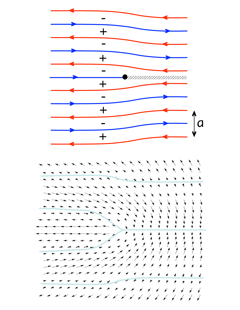
In contrast to a conventional uniform superfluid or a standard smectic density wave, here the product form of the pair-density wave LO order parameter (64) allows this composite half-integer defect. Namely, although the superfluid and the smectic density wave order-parameter components each change by a minus sign (wind by a phase of ), the product LO order-parameter , Eq. (64) remains single-valued in the presence of such , fractional composite defects.
VI.2 Energetics
The energy cost of above described vortices and dislocations can be computed with straightforward extensions of standard analyses[130, 142].
VI.2.1 -vortex:
The -vortex in the LO superfluid is obtained via a solution of the Euler-Lagrange equation for
| (154) |
under the condition of a -vortex line singularity
| (155) |
located at with a unit tangent . The smectic layers remained undistorted at long scales, (equivalently ). The solution displays a qualitatively standard form, but with distortions associated with a large anisotropy ratio , that, as we demonstrated dramatically diverges at the upper-critical field . This is reflected in the anisotropy of the mass current flow around a vortex line running within the LO (smectic, xy-) layers, (a mass flow with velocity component along the smectic layer normal, ), illustrated in Fig.11. For concreteness we look at two straight vortex line configurations.
-vortex line :
For a straight vortex line running along (z-axis) above equations reduce to
| (156a) | |||||
| (156b) | |||||
which gives , where is the azimuthal coordinate angle within a smectic layer (xy-plane). The corresponding superfluid “velocity” for such a -vortex line directed along (flowing in the xy -plane) is isotropic, given by a standard form
| (157) |
Integrating the kinetic energy density, Eq. (144b) in a system of dimensions we readily find the energy to be given by the familiar 3d (linear-logarithmic) form,
| (158) |
diverging linearly with vortex line’s length, and logarithmically with systems in-plane extent .
-vortex line :
In contrast, a vortex line directed along the smectic layers (taken here to be along the -axis, with flow confined to the anisotropic plane) characterized by
| (159) |
is described by and a velocity field
| (160) |
illustrated in Fig.11.
As expected from the superfluid-stiffness anisotropy near , where , the superflow around a vortex falls off much more slowly across the LO layers (along ) than within them (along ). This leads to (near a highly) anisotropic elliptic-like superflow with the major axis oriented along the LO layers normal (along ) and the velocity flow that is not everywhere tangent to the equipotential flows, as illustrated in Fig.11.
Substituting this flow inside the Hamiltonian (144b), the corresponding vortex energy is then readily shown to be given by
| (161) |
In 2d it reduces to a familiar logarithmic form by replacing the factor by the sample thickness.
VI.2.2 -dislocation:
An integer dislocation defect in the LO superfluid is similarly obtained via a solution of the Euler-Lagrange equation for , obtained by minimizing Eq.144b, with a condition of (equivalently )
| (162) |
and the singularity and continuity conditions
| (163a) | |||||
| (163b) | |||||
with the singular strain
| (164) |
and the dislocation “charge” density
| (165) |
As for the vortex, parameterizes the ’th dislocation loop, is the conformation of that loop, is its local unit tangent, and is the number of excess layers associated with the dislocation. Note that is independent of , since the charge of a given dislocation line is constant along the line defect.
The dislocation solution is most straightforwardly obtained in Fourier space, where equations reduce to:
| (166a) | |||||
| (166b) | |||||
and the general solution is given by
| (167) |
with a smooth elastic distortion around the dislocation line obtained via the Euler-Lagrange equation, (162), and is given by
| (168) |
The superfluid phase remains uniform at long scales, (equivalently ). In above we defined the inverse of the LO phonon propagator
| (169) |
with , a length characterizing the LO domain-wall deformations. Inserting above expression for into the original elastic Hamiltonian Eq.144b gives the Coulomb gas-like Hamiltonian that determines the energy of an arbitrary dislocation configuration
| (170) |
where is the in-(xy) plane transverse projection operator, with indicating projection onto the smectic layers. In above we also added dislocation core energy determined by its short-scale () configuration, at which above continuum analysis no longer applies. A simplest estimate (up to possibly nontrivial dimensionless factors set by , that can only be determined through a microscopic calculation) of this core energy density is given by .
In 3d, two limiting dislocation line configurations are the screw and edge dislocations,
| (171a) | |||||
| (171b) | |||||
running perpendicular to and along smectic layers, respectively. Within above harmonic continuum approximation, the long-scale elastic contribution (first term in (170)) to the energy of a screw dislocation vanishes identically (due to ), physically because of smectic’s soft in-plane curvature elasticity and due to the absence of long-scale compressional distortion in a screw dislocation, as can be readily verified. Thus its energy is determined by short-scale core energetics inaccessibility to harmonic elastic analysis.
For a single edge dislocation along (171b) , giving for the elastic part of the energy
| (172a) | |||||
| (172b) | |||||
| (172c) | |||||
where the factor of came from the regularized identity . Although the first “elastic” contribution in Eq. (170) no longer vanishes, the above energy is dominated by the short cutoff scale, and therefore in principle indistinguishable from the core energy. Thus, based on this analysis we can only provide an estimate of the 3d dislocation energies,
| (173a) | |||||
| (173b) | |||||
diverging linearly with its length.
Correspondingly, as first demonstrated by Toner and Nelson[142], in two dimensions the energy of a smectic edge dislocation is constant, i.e., system length independent, given by
| (174) |
As we will see in the next section, this observation has crucial implications for the instability of a finite temperature 2d LO state[142].
VI.2.3 half-integer vortex-dislocations defect:
As discussed above[112], on general grounds a LO (but not a FF) superconductor allows novel half-integer defects that are a composite of a -vortex and -dislocation, illustrated in Fig.10. The form and the energy associated with this defect requires a solution of Euler-Lagrange equations for
| (175) |
with singularity conditions
| (176a) | |||||
| (176b) | |||||
for concreteness taken to be a straight vortex line in running parallel to LO layers, along the axis, and .
Solving above equations gives the defect’s shape from which the energy is readily computed
| (177) |
Because the energy scales as a square of the defect’s topological charge , as expected, the above energy of the half vortex-dislocation defect is one-quarter of the sum of the energies of the unit vortex and dislocation.
VI.3 Dual description: coupled xy-smectic models
In characterizing phases in terms of topological defects, it is often useful to have a continuum field-theoretic description of defects and of the corresponding transitions associated with their unbinding. Such a description, that complements the LO Goldstone model, (144) is obtained through a duality transformations that we develop here. In 3d the analysis is somewhat complicated and results in two coupled gauge theories, whose derivation and analysis we leave to a future publication[151]. Here, for simplicity we will exclusively focus on two dimensions.
To this end, starting with , (144b), allowing for singular configurations of (vortices) and (dislocations) discussed in the previous subsection, and integrating out the smooth parts of Goldstone modes, we obtain a Coulomb gas description of a finite density of topological defects
| (178) | |||||
where
| (179a) | |||||
| (179b) | |||||
In above, are the Fourier transforms of the vortex and dislocation densities , , with , and the independent elementary integer defects, defined in the previous subsection. In above we also introduced the vortex and dislocation core energy to account for short scale core physics not accounted for by the above continuum description. Although by time-reversal symmetry the core energies of the elementary defects are identical, those of the vortex and dislocation composites will generically be distinct with .
To obtain a continuum description of these integer-valued fields, it is convenient to decouple interaction of these defects using a Hubbard-Stratonovich transformation by introducing a pair of dual real fields (corresponding potentials) with the Hamiltonian
| (180) | |||||
where
| (181) |
The thermodynamics is characterized by a partition function
| (182a) | |||||
| (182b) | |||||
where we chose to measure all energies in units of . The summation over vortex and dislocation charges can be readily done in the dilute defect limit, corresponding to large core energies . In this limit the summations can be limited to nine lowest order terms, corresponding to no vortices present, , one vortex of either species and sign at a site, , or two vortices of distinct species sitting at a single site, . Equivalently, in terms of vortex-dislocation nomenclature, these respectively correspond to
This gives
| (184) | |||||
All other vortex configurations (for example two defects of either species sitting on distinct sites) are not included as they correspond to higher order contributions, suppressed at low fugacity. After re-exponentiating, above leads to a generalized sine-Gordon model for the coupled fields, with the dual Hamiltonian
| (185) |
where the couplings are , and , and we converted the sum over into an integral over via a lattice constant .
In the opposite limit of a small core energy, the defect density is high and the summation over the integer charges can be carried out utilizing the Poisson summation formula, that leads to a replacement of the e.g., potentials above by the Villain potential, defined by:
| (186a) | |||||
| (186b) | |||||
The latter can be approximated by a single harmonic with an effective coupling .
The resulting generalized sine-Gordon model is convenient for analyzing the effects of defects on the LO state, particularly for the computation of their screening on long scales, unbinding, and for the analysis of the resulting disordered state. From the form (185) it is clear that (aside from an inconsequential anisotropy) the dual vortex sector described by has a standard sine-Gordon form. In contrast, the dual dislocation sector, described by is qualitatively modified by the highly nonlocal and qualitatively anisotropic smectic kernel, [169].
We next turn to a detailed discussion of implication of these defects for possible phases and transitions associated with the LO state.
VII Phases and Phase transitions: Larkin-Ovchinnikov liquid crystals
We now turn to a discussion and characterization of a class of phases emerging from the Larkin-Ovchinnikov state by a partial disordering of it. Because these phases partially break spatial symmetries, we will refer to them collectively as LO liquid crystals. We first discuss general symmetry based possibilities and then explore their concrete realization in terms of fluctuation-driven proliferation of topological defects.
VII.1 Landau’s order parameters and spontaneously broken symmetries
A conventional characterization of phases is through the Landau’s classification, where phases are distinguished by non-vanishing order parameters and corresponding symmetries that they break. From this prospective a zero-temperature LO (smectic pair-density wave) superfluid () breaks three symmetries: the translations along (), the rotations about the axis transverse to (of the full 3d Euclidean group ), and the symmetry associated with atom conservation. The corresponding non-vanishing order parameter, that transforms non-trivially under these group of symmetries is the LO pair-density wave (64).
By considering all possible basic combinations of spontaneously broken subset of these symmetries, we uncover five additional atomic liquid crystal phases, that are descendants of the smectic LO state[170]. To enumerate these systematically we begin with the zero-temperature LO state, where all three above symmetries are broken and partially restore them by progressively disordering the state. Restoring the translational symmetry , while keeping and leads to a state with orientational and off-diagonal orders, that is a nematic superfluid, . By analogy with the conventional (non-superfluid) nematics the resulting state can be characterized by a complex traceless symmetric second-rank tensor .
Subsequently disordering the orientational order and thereby also restoring the rotational symmetry leads to an isotropic superfluid, , that exhibits a finite species imbalance. Symmetry-wise the resulting state is isomorphic to the polarized superfluid, predicted[44, 4] and observed to appear at a nonzero imbalance on the BEC side of the BCS-BEC crossover. In contrast, (as a descendant of the LO state expected to be stabilized by Fermi surfaces imbalance) here the state is realized in an imbalanced superfluid on the BCS side, something that has been searched for dating back to Sarma[75], but has not been possible within mean-field treatments, that instead predict an instability to phase separation[40, 44, 4].
As summarized by Tables 1,2 the additional three phases, smectic, nematic and isotropic Fermi liquids, are the non-superfluid counterparts of the three discussed above, obtained by first restoring the symmetry by disordering the off-diagonal long-range order. The fully disordered state is simply the normal state of the polarized Fermi gas, albeit strongly interacting. Together these intermediate fluctuation-induced phases (along with a number of other possible ones that we discuss below) naturally interpolate between the fully gapped singlet (homogeneously and isotropic) BCS superconductor at zero imbalance and low temperature, and the normal polarized Fermi liquid at large imbalance and/or high temperature.
| U(1) | U(1) | U(1) | ||
| phases | |||
| X | |||
| X | X | ||
| X | |||
| X | X | ||
| X | X | X |
VII.2 Larkin-Ovchinnikov liquid crystals via topological defects unbinding
A complementary way to characterize phases and phase transitions between them is in terms of topological defects proliferation[141]. For conventional phases and transitions (e.g., 3d xy or Ising models) this is simply a complementary description that is sometimes convenient. However, for topological phases, where Landau order parameter is unavailable or just insufficient to distinguish two phases, this defect-proliferation approach is indispensable and therefore superior to the order-parameter Landau’s “soft-spin” description. One prominent and familiar example is the description of the low-temperature quasi-long-range ordered phase of the 2d xy model and its disordering. In this case, both the low- (“ordered”) and high-temperature (disordered) phases exhibit a vanishing xy order parameter, and are respectively only topologically (not symmetry) distinguished by bound and unbound vortex defects and by the associated behavior of the correlation functions (power-law and exponential, respectively)[141].
With this in mind, we characterized the LO and its descendant states in terms of a proliferation of the four types of topological defects , introduced and analyzed in Sec.VI.
As discussed above, at the LO phase is characterized by long-range off-diagonal and translational order and is thereby distinguished by a nonzero LO order parameter . In this ground state all of the above topological defects are absent, confined into topologically neutral pairs.
VII.2.1 3d phases and transitions
Although, (as we explicitly demonstrated in Sec.V) at nonzero temperature the LO order parameter vanishes in 3d (and in 2d), the 3d LO phase is distinguished from its more disordered descendants by the absence of unbound topological defects, in direct analogy with the quasi-long-range ordered state of the 2d xy model. Thus, in this same sense at nonzero the 3d LO smectic is a topologically ordered (but phonon, elastically disordered) phase.
Upon increasing temperature, or decreasing the stiffnesses (e.g., by tuning the strength of the Feshbach-resonant interactions, or by adjusting the fermionic species imbalance), one or more of the four topological defects will proliferate, thereby leading to a transition of the LO smectic (PDW) into one of its descendants. The actual sequence of defects unbinding is determined by the relative energetics, given by Eqs.(161),(173),(177). Lacking a reliable calculation (throughout the phase diagram) of dependences of the stiffnesses on the experimentally tunable parameters (, imbalance , interactions , and the number of atoms), the phase diagram can only be qualitatively mapped out in terms of the three effective stiffnesses . In the thermodynamic limit (, not necessarily relevant to atomic traps; see below), the relative defects energetics is quite unambiguous:
| (187) |
where for simplicity we ignored anisotropies in . Based on this energetics one may be tempted to conclude that in this limit (unless preempted by a first-order transition) it is the integer dislocation loop defects that proliferate first and the LO smectic preferentially disorders into a nematic superfluid, . However, in contrast to the 2d KT mechanism[141], the 3d disordering transitions take place when the relevant stiffness, renormalized by quantum and thermal fluctuations is continuously driven to zero at the transition, or takes place at a finite (rather than a vanishing) fugacity. For a thermal transition this roughly corresponds to a transition temperature set by the corresponding stiffnesses, and .
Lacking a detailed quantitative theory of such 3d transitions we can only construct a qualitative phase diagram, that we display in Fig.4. It summarizes all basic phases that naturally appear upon disordering of the LO smectic superfluid by unbinding four fundamental type of topological defects discussed above. One important physical input is the observation that increasing the Zeeman energy, (or equivalently, the species imbalance, ) toward the normal Fermi liquid state, at , predominantly leads to a suppression of the superfluid stiffness and therefore to a destruction of the SF order. Conversely, a reduction of the Zeeman field (and species imbalance) toward a conventional isotropic and homogeneous superfluid at , primarily leads to a reduction of the elastic moduli of the smectic pair-density wave by increasing its period and thereby weakening the interaction between the LO domain-walls (see Eq. (97b)). Thus lowering of is expected to predominantly suppress, i.e., melt the positional smectic order.
Thus, starting with the LO state and decreasing leads to the unbinding of the integer dislocations , and a transition to an orientationally-ordered, i.e., a nematic “charge”-4 superfluid, . The later “charge”-4 feature of naturally appears as the remaining secondary order parameter once the LO positional order is destroyed by unbinding of integer dislocation loops. General arguments predict a subleading singularity of at the continuous transition between and . Since in contrast, the “charge”-2 SF nematic order vanishes in the LO state, a direct transition to it from the LO state can generically only proceed through a first-order transition.
Conversely, we expect that increasing starting with the LO will lead to a suppression of , a proliferation , and a transition to a -smectic Fermi liquid, , a non-superfluid periodic state with a wavevector that is twice the LO state. Alternatively, as suggested by the energetics in Eq. (187), it maybe that the lower-energy half-vortex dislocation defects (or the , but not both) unbind first, in which case a transition to a nematic Fermi liquid, (with the restored translational and U(1) charge symmetries) takes place. The resulting state is qualitatively distinct from the more conventional nematic (orientationally ordered) phase in which both and are proliferated. Both are also distinct from the nematically ordered state, in which only integer dislocations, and integer vortices, are unbound. One can envision a number of other states and phase transitions at low by further considering the disordering of the nematic superfluid, by unbinding various patterns of disclinations and -vortices. We leave a more detailed analysis of these to a future study.
VII.2.2 2d phases and transitions
The nature of the phase diagram changes qualitatively in two dimensions at nonzero temperature. Based on the work of Ref.142 (in the context of conventional smectic liquid crystals) and from the analysis in Sec.VI.2, that shows a finite energy cost of a 2d smectic dislocation, we conclude that at any nonzero in 2d, the dislocations proliferate, thereby destroying the LO () phase. It is replaced by a homogeneous, but quasi-orientationally-ordered, “charge”-4 superfluid nematic, . Upon rotation this superfluid will display “charge” vortices (), that, because of its nematic order we expect to form a uniaxially distorted hexagonal lattice. Upon changing , , , the nematic superfluid can then undergo further disordering transitions toward a polarized Fermi liquid and an isotropic (e.g., BCS) superfluid. In particular, we expect two Kosterlitz-Thouless transitions associated with the loss of 2d superfluid and orientational (nematic) quasi-long-range orders. Because and therefore vanishes strongly near , we expect the superfluid KT transition to precede the nematic-isotropic one.

VII.3 Fractionalized phases and topological order
In above discussion we argued for the existence of at least three topologically distinct Fermi liquid phases that naturally emerge from disordering of the LO () phase by unbinding different combinations of allowed defects. Because, as demonstrated above the conventional vortex and a conventional dislocation are composites of the fundamental defects the nonsuperfluid states , and their isotropic cousins , (in which disclinations are also unbound) are expected to be “fractionalized”[171], topologically distinct from their conventional Fermi liquid analogs, where are also unbound.
These novel phases are analogous to the putative phase-disordered fractionalized states obtained by unbinding double () vortices, studied extensively by Sachdev, and by Balents, Senthil, Fisher, and collaborators[172, 173, 171] in the context of high temperature superconductors. The resulting nonsuperfluid phase is distinguished from a conventional Fermi liquid by a gapped “vison”, a defect that is a remnant of the fundamental vortex after the composite (double) vortices proliferate. These states are also characterized by “fractionalized” charge-neutral spin-1/2 bosonic and charge-e spinless fermionic excitations.
The states , also bare a close relation to the collective mode fractionalization discussed by Sachdev, et al. [174, 175, 176] in the context of quantum paramagnetic phases, emerging from disordering a collinear spin-density wave. As with the LO state, where the order parameter is a product of the superfluid and smectic order parameters, Eq.(64), there too the order parameter is of product form, encoding spatial modulation of the spin density, and therefore admits half-integer (vison-like) defects.
As we have seen in the previous subsection, a characterization of both the conventional and the fractionalized (topologically ordered but otherwise disordered) phases can be faithfully formulated directly in terms of distinct patterns of proliferation of the four types of vortex and dislocation defects, listed in Eq. (151). It can also equivalently be done in terms of a dual sine-Gordon (and in 3d gauge-theory) model , Eq. (185). We now present a complementary effective Ising gauge theory description, that can sometimes be convenient. In the absence of an underlying rotational invariance (that otherwise has been our focus throughout) and for simplicity ignoring anisotropy of the striped LO state, all the phases and transitions can be captured by a Euclidean action (in space-time )
| (188) |
where the Ising gauge field, couples to the bosonic (rotor) matter fields , and its nonzero flux through a plaquette encodes the presence of a half-integer defect. The gauge field encodes the local Ising redundancy of splitting the LO order parameter (64) into a “charge”-2 boson, , that creates a zero-momentum Cooper-pair (diatomic molecule) and a neutral boson, , that creates a density wave at a LO wavevector . Formally, the gauge field can be introduced as a Hubbard-Stratonovic field that decouples the LO order parameter into its charge and density wave parts. The variety of phases and transitions between them are summarized in the phase diagram, Fig.4 and a flow-chart, Fig.12.
In above formulation, the LO superfluid () is a state at large and arbitrary , in which both and are Bose-condensed, and is gapped through a Higg’s mechanism. In this state, gapped vortices in and respectively correspond to the superconducting vortex and the integer dislocation, that we discussed in the previous subsection.
For small and large vortices in proliferate, driving normal and restoring the (atom conservation) symmetry, while keeping condensed. A large forces a vanishing Ising flux with , that corresponds to a gapped vison. The resulting nonsuperfluid state is deconfined in a sense that that it exhibits a gapped bosonic excitation carrying an Ising charge and thereby acquiring a phase upon encircling a vison. In our earlier notation this is the nonsuperfluid periodic state we dubbed , in which vortices have proliferated, but dislocations remain bound. Lowering drives visons gapless, corresponding to a proliferation of the fractional defects that induces a transition to the homogeneous but orientationally ordered (nematic) nonsuperfluid state, . We note that condensation of in the presence of unbound defects automatically also leads to a proliferation of defects and therefore (aside from the nematic conventional order) the resulting is fully disordered.
In the opposite regime of large and small vortices in proliferate, driving normal and restoring the translational symmetry, while keeping condensed. For large vison remains gapped and the resulting superfluid homogeneous state exhibits gapped density excitations , carrying an Ising charge and nontrivial statistics with the vison. The resulting state is the charge-4 nematically ordered superfluid, . Upon reducing visons proliferate, driving a transition to through this alternate route.
In contrast to lowering , the transitions out of the and states at large can be driven by respectively lowering and and thereby unbinding the second set of integer defects, and , respectively. Since visons remain gapped, the resulting nonsuperfluid nematic state is the topologically ordered , qualitatively distinct from . The deconfinement transition - is then driven by lowering through a condensation of visons and is in the inverted Ising universality class.
A naive attempt at a generalization of the above Ising gauge theory action, (188) to the rotationally invariant smectic form suggests a replacement of the operator by a gauge-invariant lattice Laplacian. However, on general grounds, without fine-tuning such Ising lattice form appears to preclude a fully rotationally-invariant formulation necessary for a fully-rotationally invariant LO (superfluid smectic) state.
Finally, we note that above orientationally ordered state can further disorder into isotropic states by proliferation of disclinations. We leave a more detailed study of these phases and the corresponding transitions to future research.
VIII Fermions
So far all of our discussion following the defining microscopic model in Sec.II has been confined to the bosonic sector of the Larkin-Ovchinnikov state. The resulting low-energy quantum thermodynamics is encoded in the Hamiltonian, , Eq.(77c) (and the Lagrangian , Eq.(88)) for the superfluid phase and smectic phonon Goldstone modes. In contrast to the fully gapped superconductors where this is sufficient at low energies, the gapless nature of the LO state also requires the inclusion of gapless fermionic excitations for a complete description of the state. While a detailed analysis of these is beyond the scope of the present manuscript, below we comment on a few a key features of the fermionic sector of the LO state.
VIII.1 Gapless fermionic excitations in the Larkin-Ovchinnikov state near
As we have seen in our discussion of the Goldstone modes, there are two complementary descriptions of the FFLO states, respectively valid near and . Just below at the continuous FL-FFLO phase the pairing order parameter, is small with a weak sinusoidal modulation, and the momentum-space description is most appropriate. The corresponding mean-field many-body wavefunction for e.g., the FF state is given by Eq.(20). It is of the BCS form with a range of over which the energy of the corresponding Bogoliubov quasi-particles is driven negative by the Zeeman field. These therefore form a Fermi sea with all the phenomenology associates with the gapless fermionic excitations at the Fermi surface.
For a more general FFLO state defined by a set of reciprocal lattice vectors , no exact analytical solution of the BdG Hamiltonian is available. The periodic couples all particle (atoms) and hole states connected by the reciprocal lattice , leading to an anomalous -dependent band structure of Bogoliubov quasi-particles.
However, some progress can be made for a purely sinusoidal LO state with only reciprocal lattice vectors. As discussed earlier a BCS-like mean-field Hamiltonian for such a state is given by
| (189) |
The difference from the FF BCS Hamiltonian, analyzed exactly in Sec.II is in the appearance of both and Fourier components of , taken to be equal for the simplest cosine LO form. These couple each creation operator to two fermionic atom annihilation operators and , with each in turn coupling to another set of two operators at different ’s, thereby generating an infinite-dimensional space that needs to be diagonalized. Focusing on the three-dimensional subspace for each , the Hamiltonian can be rewritten in the following Bogoliubov–de Gennes form:
| (190) | |||||
with the three component generalization of the Nambu spinor given by
| (191) |
and the corresponding Bogoliubov–de Gennes Hamiltonian matrix. The nontrivial eigenstates encode that the excitation in the LO state is a linear combination of a hole , an atom , and an atom ).
Although it appears that the problem reduces to a diagonalization in this three-dimensional subspace, in fact (in contrast to the single Fourier component FF state, where is block-diagonal, here) there is a coupling between a bottom component of a spinor and the top component of the spinor ,
| (192) |
This leads to the aforementioned infinite-dimensional space to diagonalize, corresponding to the band structure of the Bogoliubov quasi-particles, analogous to a system with a diagonal periodic potential.
Despite these complications, for a large enough (such that , well satisfied near where ) an approximate treatment is possible because the coupling is dominated by the degenerate particle-hole states near the Fermi surface, which reduces the problem to only a pair of states for every value of . For positive (negative) the pair is the top (bottom) two components of the spinor , leading to a Cooper-pair with () center of mass momentum.
Diagonalizing the BdG Hamiltonian then leads to two sets of the Bogoliubov quasi-particle operators ,
| (193a) | |||||
| (193b) | |||||
| (193c) | |||||
| (193d) | |||||
with the corresponding four branches of excitation spectrum,
| (194a) | |||||
| (194b) | |||||
| (194c) | |||||
| (194d) | |||||
, and the coherence factors , , approximately given by the FF expressions in Eq. (15). In the first [second] pair of equations, Eqs.(193a),(193b) [Eqs.(193c),(193d)], the particle-hole hybridization is via [], as for the FF state.
As demonstrated for the FF state in Sec.(II), it is clear from the spectra , Eq. (194), that the LO state exhibits regions of both gapped and gapless fermionic excitations, with closing of the gap driven by a combination of the Zeeman (imbalance) energy and the Doppler shift . For pairing driven by () the gapless states appear at the minimum of the () located in a wedge around (), where for positive , () is driven negative. The LO ground state thus takes the form given in Eq.(20), exhibiting Fermi pockets of Bogoliubov quasi-particles, with a Fermi surface of gapless excitations defined by , as illustrated in Fig.13.
In the complementary wedge of around , i.e., running along the LO stripes given by the nodes of the LO order parameter, the superconducting gap remains finite, growing to its maximum value (suppressed by ) as
| (195) | |||||
The quadratic dispersion along the stripes is characterized by an enhanced effective mass .
While above analysis gives some understanding of the LO states, it is approximate and does not address the detailed nature of a more generic LO-like states. These may be understood by self-consistently diagonalizing the BdG equations in real space. An estimate of the mean-field BCS-LO and LO-FL phase boundaries requires a computation of the total energy as was done in Ref.4 for the FF state. A complete solution for the LO state requires a numerical analysis[95, 96, 97].
VIII.2 Gapless fermionic excitations in the Larkin-Ovchinnikov state near
The above calculation of the LO quasi-particle spectrum near can be complemented by a treatment valid near . At low , the LO order parameter is given by a periodic (period ) array of domain-walls of width [95, 96, 97, 98], rather than a single harmonic.
The form of the quasi-particle excitations is determined by a two-component Nambu wavefunction satisfying the BdG equation
| (196) |
where and we took the order parameter to be real (characteristic of the mean-field LO state) stripe domain-walls lying in the plane, with the normal along , and approximated the chemical potential by a Fermi energy , valid deep in the BCS regime. In a matrix form, the BdG equation is given by
| (197) |
For a striped LO state we can utilize translational invariance along the stripes, , taking , with satisfying
with the effective 1d Fermi energy.
The low-energy spectrum is determined by the excitations near the Fermi energy
| (199) |
with and the envelope wavefunctions satisfying
| (200) |
For sufficiently large, so that we can linearize around the Fermi points by neglecting the quadratic correction to the dispersion, , we obtain
For a single “- to +” domain-wall the solution can be readily found[177, 178] and exhibits two normalizable Andreev zero-energy bound states,
| (202a) | |||||
| (202b) | |||||
where is the effective coherence length (setting the width of the bound state) and in the second line we approximated the “- to +” domain-wall by a step function valid for . For the opposite sign “- to +” domain-wall, the normalizable Andreev zero modes are given by identical expressions, but with the reversed sign in front of the in the second component of the Nambu spinor.
The minimum excitation gap is determined by the nonlinear correction to the free spectrum, the perturbation , that we incorporate through a degenerate perturbation theory in the two-component degenerate subspace of Andreev zero modes, . A simple computation gives the off-diagonal matrix elements , splitting the Andreev zero modes to , with
| (203a) | |||||
| (203b) | |||||
The maximum of the gap can be estimated through a variational solution of the Eq.(200) for the nondegenerate case of , giving
| (204a) | |||||
| (204b) | |||||
for the width of the state localized on the domain-wall and the maximum of the gap.
For a periodic array of domain-walls with period (the LO state), the coupling between the Andreev states localized on each domain wall splits their energy into bands separated by gaps and dispersing with . The eigenstate for the bottom of the band, can be obtained by generalizing the single domain-wall zero-energy state, Eq.(202) to a periodic array . The solution for the bottom of the Andreev band is simply a sum of two periodic arrays of states, localized on “- to +” (at ) and on “+ to -” (at ) domain-wall arrays, respectively
| (205) |
For a nonzero chemical potential difference (Zeeman energy) to impose the spin imbalance, the spin up excitation spectrum (203b) simply uniformly shifts down by . exceeding the minimum gap , Eq.(203), generically induces Fermi pockets (Fig.13) of the Bogoliubov quasi-particles centered around out to [179]. As expected (from the fact that these are different regimes of the same LO phase) the above outlined spectrum is in a qualitative agreement with that near , found in the previous subsection.
VIII.3 Fermion-Goldstone modes coupling in the Larkin-Ovchinnikov state
As discussed above, the LO state is characterized by a simultaneous presence of gapless Goldstone modes (particularly “soft” for the fully rotationally invariant geometry of an isotropic trap) and gapless fermions. Consequently, for a complete description a coupling between these must be included. These can in principle be derived from the microscopic BCS Hamiltonian evaluated inside the LO state beyond a conventional mean-field treatment. Alternatively, the fermion-Goldstone mode couplings can be simply deduced based on symmetry considerations. The leading ones include, the coupling of the supercurrent and of the LO phonon to the quasi-particle current and number density, and are given by
| (206a) | |||||
| (206b) | |||||
Because atom number conservation is effectively “broken” in the superfluid LO state, above couplings must be supplemented by the anomalous (number violating) operators, such as e.g., . Effects of these interactions on the fermionic and collective bosonic () spectral functions requires a detailed analysis, that parallels studies of gauge fields[180, 181, 182, 183, 184, 185], Goldstone modes [117] and critical modes[186, 187] coupling to electrons in gapless superconductors and metals. A preliminary analysis suggests that in the LO state these derivative couplings (enforced by the underlying gauge and spatial symmetries) only lead to a finite renormalization of model’s parameters as well as Landau-like damping of the Goldstone modes. In addition to the above symmetry-dictated couplings, the presence of gapless fermions can generate Berry’s phase terms[155], that can qualitatively modify the conventional LO phonon dynamics derived in Sec.III.4. We leave a detailed study of these interesting questions to future research.
IX Larkin Ovchinnikov states in a trap
The primary experimental application of our results is to polarized paired superfluidity in trapped degenerate atomic gases. It is thus crucial to extend our bulk analysis to take into account the effect of the trapping potential , that in a typical experiment is well-approximated by a harmonic-oscillator potential. While a full analysis of the effect of the trap is beyond the scope of this manuscript, in the present section we study this problem within the well-known local density approximation (LDA). We note that several recent studies (e.g., Refs. 52, 55, 44, 4, 56, 57, 58, 60, 61) have also addressed polarized superfluidity in a trap.
IX.1 The local density approximation
Much like the WKB approximation, LDA corresponds to using expressions for the bulk system, but with an effective local chemical potential in place of . The validity of the LDA approximation relies on the smoothness of the trap potential, with the criterion that varies slowly on the scale of the longest physical length (the Fermi wavelength, scattering length, effective range, etc.) in the problem, i.e., . Its accuracy can be equivalently controlled by a small parameter that is the ratio of the single particle trap level spacing to the smallest characteristic energy of the studied phenomenon (e.g, the chemical potential, condensation energy, etc.), by requiring . Within the LO state the longest length is clearly the LO period, , that near is bounded by the coherence length (that near unitarity can be as short as inter-atomic spacing , where is the trapped condensate radius and is the total number of atoms), and thus . Thus, in this regime, away from (where for a continuous BCS-LO transition the period is expected to diverge) the effects of the trap can be safely treated within the LDA.
The generalization of the model of an imbalanced resonant Fermi gas to a trap is straightforward:
| (207) | |||||
where is a fermionic field operator with a Fourier transform . Henceforth, to be concrete, we shall focus on an isotropic harmonic trap (although this simplification can easily be relaxed) with
| (208a) | |||||
| (208b) | |||||
latter expression defining the cloud size . Within LDA (valid for a sufficiently smooth trap potential , see above), locally the system is taken to be well-approximated as uniform, but with a local chemical potential given by
| (209a) | |||||
| (209b) | |||||
where the constant is the true chemical potential (a Lagrange multiplier) enforcing the total atom number . The spatially-varying spin-up and spin-down local chemical potentials are then:
| (210a) | |||||
| (210b) | |||||
with the chemical potential difference uniform.
Consequently, within LDA the system’s energy density is approximated by that of a uniform system, (17), with the spatial dependence (via the trap) entering only through . The ground state energy is then simply a volume integral of this energy density. Thus, the phase behavior of a uniform system as a function of chemical potential, , translates into a spatial cloud profile through , with the critical phase boundaries corresponding to critical radii defined by . [44, 4] As first predicted[44], this leads to a shell-like cloud structure that has subsequently been observed experimentally [34, 35, 36, 37].
Within the LDA, we can furthermore deduce the effects of the trap on the structure of the LO state. We turn to this analysis next.
IX.2 Trap-induced elastic distortion
As discussed earlier, the Larkin-Ovchinnikov state breaks translational symmetry and as other crystals thereby exhibits a rigidity to stress. Confinement in a trap induces a variation in the chemical potential that (as observed experimentally in the BCS superfluid [34, 35, 36, 37]) has the effect of expelling the imbalance (polarization) to the edge of the cloud. Since in the LO state the BCS order parameter domain walls “carry” the imbalance (the imbalanced fermions are confined to domain walls in , where their cost is minimum), in the LO state the increased imbalance is accommodated by the increase in the density of domain walls. Thus, the trap confinement introduces an effective longitudinal stress that acts to compress the LO state (increase its local wavevector ), where the chemical potential is reduced. This tendency is captured by introducing a local longitudinal stress, into the LO phonon Hamiltonian
Above trap-phonon coupling arises by repeating our derivation in Secs.II,III with the trap potential , treating it within the LDA. The effective local chemical potential enters through many contributions, but the leading order effect comes from a position-dependent wavevector generalization of Eq. (25)
| (212a) | |||||
| (212b) | |||||
| (212c) | |||||
In above, consistent with the LDA applicability we utilized the limit. Since , we deduce that the local stress is given by
| (213a) | |||||
| (213b) | |||||
where is the trap induced stress scale, and we inserted an additional factor of to crudely account for the breakdown of LDA based analysis near the cloud edge, where atom density, vanishes at . As expected on physical grounds, is a function that vanishes at the trap center and peaked on its outer shell set by .
With this, the distortion is given by a standard form
| (214) |
in terms of a Greens function that is a derivative of the smectic Greens function, with
| (215a) | |||||
| (215b) | |||||
From this the trap-induced imbalance distortion, is straightforwardly computed
| (216a) | |||||
| (216b) | |||||
| (216c) | |||||
with final unnecessary crude approximation by construction of and its coupling to recovering the expected result.
IX.3 Trap-induced LO 3d-2d dimensional crossover
A microscopically accurate account of the trap inside the LO state, and in particular its coupling to the Goldstone modes with appropriate boundary conditions (beyond above kludge treatment) is not currently available. Perhaps a numerical analysis (e.g., numerical solution of BdG equations or full quantum Monte Carlo simulation)[52, 56, 70] can provide the desired description.
However, lacking such first principles analysis, we are constrained to proceed phenomenologically, working directly with the effective Goldstone mode theory of . Expanding the LO state about the trap-distorted state discussed above, the distortion is again governed by the smectic Hamiltonian (144b). Although, some of the effects of the trap will enter through the position dependent elastic moduli , we expect that the leading effects of the trap are incorporated through the physically motivated boundary conditions on . Because atom density vanishes at the edge of the cloud, the LO inner shell is expected to be surrounded by an outer shell of a fully polarized normal cloud lacking any positional order. Thus, we expect Neumann boundary condition
| (217) |
( the unit normal to the cloud’s boundary) to be the most appropriate one to supplement the Euler-Lagrange equation for . However, the appearance of forth derivative along , Eq. (144b) requires that this boundary condition be supplemented by additional ones on the domain-wall normal, .
Given the cylindrical form of smectic elasticity, Eq. (144b), analytically implementing such spherically symmetric boundary conditions is quite challenging. However, because our goal here is more modest, a qualitative understanding of the trap-induced dimensional crossover can be obtained by simply using cloud size scale to cutoff long scales appearing in a bulk analysis. Technically, our analysis amounts to instead working with periodic boundary conditions and a cylindrical trap. The calculational convenience of such boundary conditions is that they do not modify the form of the eigenmodes (still Fourier modes), and enter only through a restriction on the allowed eigenvalues, , , with . Thus, length scales associated with the trap and finite cloud size, , crudely enter through the minimum allowed momentum eigenvalues (roughly set by the cloud size ), and thereby capture the spatial extent of the lowest phonon eigenmode even for correct boundary conditions.
A key observation that emerges from such treatment is that because of the “infinite” anisotropy of the bulk smectic modes in Eq. (144b), with (or equivalently ), the dimensional crossover is qualitatively different than in systems with more conventional, scaling-wise isotropic elasticity. Namely, examining smectic bulk propagator , it is clear that unless , the phonon fluctuations will not be controlled by bulk modes. That is, as illustrated in Fig.19, for any reasonably shaped trap (even quite anisotropic one, other than an extremely anisotropic with ), fluctuations will be controlled by the dimensional “zero” modes, , that are uniform along the axis, representing compression-free LO undulations. Indeed this is allowed because of the expected Neumann boundary condition on , that allows a zero-energy cost rigid displacement along of the LO domain-walls.

To demonstrate above expectation, we account for these “zero” modes by using a generalized mode expansion of that explicitly includes the -independent modes
In terms of these the Hamiltonian becomes
and can be used to calculate smectic phonon fluctuations. For example using and equipartition, local root-mean-squared (rms) fluctuations are given by
| (220a) | |||||
| (220b) | |||||
| (220c) | |||||
| (220d) | |||||
where in the second line we approximated mode sums by integrals in a standard way. Indeed as summarized by (220d), by comparing the two (bulk and zero mode) contributions to , as anticipated on general grounds above it is clear that for isotropic (and even highly anisotropic) traps, the “zero” mode second contribution dominates as long as .
Applying this to a spherically symmetric trap with , we conclude that indeed fluctuations are controlled by the “zero”-mode LO phonons. We thus conclude that all the correlation-function properties of the LO state will be even more anomalous, characterized by a dimensional zero-mode action, that at a harmonic level is given by
| (221) |
More detailed implication of these observations, particularly in contexts of specific experimental geometries remain to be explored. We hasten to add, however, that by equipartition, the finite temperature the LO thermodynamics will nevertheless be dominated by bulk modes, simply due to their bulk-to-surface dominance.
X Experimental implications
There is a large number of experimentally observable effects, that emerge from our study. A comprehensive treatment of these requires further extensive studies, that lie outside the scope of the present manuscript. Here we simply sketch out a few of the most important experimental signatures of our predictions.
X.1 Larkin-Ovchinnikov order parameter
As discussed in the Introduction and in Sec.V, at finite temperature in the thermodynamic limit (see below for the discussion in the trap) isotropically-trapped Larkin-Ovchinnikov phase is characterized by a vanishing average LO order parameter, i.e., . Reminiscent of 2d superfluids and crystals[130, 141], this is a reflection of its enhanced thermal fluctuations. As with these well-known examples and other topological phases, this does not however imply that the state is unstable (at least not in 3d), but that it requires a finer characterization (e.g., correlation functions, topological defects, etc.) beyond a simple Landau order parameter. One of the experimental implications is, that, consequently the leading nonzero Landau order parameter characterizing the LO state is the translationally-invariant “charge”-4 (4-atom pairing) superconducting order parameter, , introduced in Eq. (70a). Thus, in the presence of thermal fluctuations the LO phase corresponds to an exotic state in which the off-diagonal order is exhibited by pairs of Cooper pairs, i.e., a bound quartet of atoms, rather than by the conventional 2-atom Cooper pairs[119]. In 2d and 3d this higher order pairing is driven by arbitrarily low- fluctuation, rather than by a fine-tuned attractive interaction between Cooper pairs, and therefore akin to 2d superfluids and crystals has no mean-field description. While a direct experimental probe of may be challenging, enhanced fluctuations in the LO state can be directly observed through correlation functions to which we turn next.
X.2 Momentum distribution function
Probably the most striking signature of the LO state is the novel form of the Cooper-pair momentum distribution function, . As for a conventional resonantly-paired superfluid, should be accessible by a detuning sweep (controlled by a magnetic field) that projects the finite-momentum LO Cooper pairs on the BCS side onto tightly bound molecules on the BEC side of the Feshbach resonance[7], and then observed through a standard time-of flight imaging of the resulting molecular condensate. In contrast to a conventional bosonic and BCS condensates (that in a trap display a single peak, associated with a condensation into a lowest trap state, or its interaction-swelled equivalent), the LO condensate is expected to display a spontaneous reciprocal lattice of condensate peaks associated with its periodic structure, Fig.20.
While in mean-field approximation is predicted[53, 44, 4, 112] to resemble a superfluid in an optical periodic potential[188, 1], the spontaneous nature of its translational and orientational symmetry breaking, in the presence of thermal fluctuations lead to important qualitative distinctions. Although the full anisotropic form is quite complex and best evaluated numerically, the asymptotic form of can be readily obtained analytically. As calculated in Sec.V, exhibit a power-law (algebraic) peaks around harmonics of the ordering wavevector , replacing the mean-field -function Bragg peaks of bosons in a periodic potential[188, 1]:
| (222) |
where for simplicity we specialized to , the form factor is given after Eq. (124) and . This form is reminiscent of (1+1)d Luttinger liquids and two-dimensional crystals[136, 137, 138, 141], and is a reflection of the quasi-long-range order of the nonzero-temperature 3d LO state. While physically quite distinct, is mathematically closely related to the structure function of a conventional smectic[134, 129]. Another feature of is the absence of the condensate peak, that qualitatively distinguishes the LO state from a supersolid[87, 88, 89, 90], where crystalline and superfluid orders merely independently coexist. We expect these novel features to be the smoking gun for the LO state, in principle observable in time-of-flight imaging.

X.3 Structure function
The density-density correlations, conventionally measured in the reciprocal space using x-ray or neutron scattering is another important quantity that can be experimentally probed. The simplest is the static structure function, that, using is straightforwardly computed (see Sec.V):
| (223a) | |||||
| (223b) | |||||
where for simplicity we evaluated it at and is a form factor. contrasts with by its insensitivity to the off-diagonal (i.e., superfluid) order. In three dimensions it also displays quasi-Bragg peaks, but at twice the reciprocal lattice vectors, , with the fluctuation exponent, and just like conventional smectics[135, 129, 130] (unlike ) does exhibit the peak.

After a projection onto the molecular BEC state, a density profile for a large atomic cloud should be measurable in situ. Computing a Fourier transform of its correlations then allows one to test , above. This way, in principle the dynamic structure function (a Fourier transform of two-time density correlation function) should also be accessible.
Alternatively, the dynamic structure function can be directly measured using Bragg spectroscopy[157, 158, 159], with its static limit obtained by integrating over frequencies. Based on successful measurements of the Bogoliubov mode in bosonic condensates[158, 159], we expect that the peaks in the (associated with its poles) can be used to give the dispersion of the collective modes, the superfluid phase and LO phonon ,
| (224a) | |||||
| (224b) | |||||
with the corresponding lifetimes remaining to be determined.
Related to the dynamic structure function is the generalized density and polarization (spin-imbalance) response function to a periodic potential. The periodic nature of the LO state makes it possible to use a perturbation at half the wavelength of the LO state to resonantly excite long-scale collective modes, such as the polarization-dipole mode, that can be readily detected in a trapped gas. This was proposed and carefully investigated for a 1d LO state in Ref.189 and should also apply in the two and three dimensional cases considered here. We leave the analysis of these and related experiments to a future more detailed study.
X.4 Trap effects
As is clear from the discussion in Sec.IX a detailed study of the effects of the trap is essential for an explicit contact with experiments. By introducing system boundaries, a trap modifies the structure of and fluctuations in the LO state, that, away from (where LO period can potentially diverge[102, 96]) can be treated within LDA.
X.4.1 Fluctuations
The detailed phenomenology of the LO state in a trap depends on the nature of the boundary conditions, that still remain to be understood. However, for large atomic clouds with small surface to volume ratio, the boundary effects are expected to be a weak perturbation to the bulk. As discussed in Sec.IX, in this case its effects can be taken into account phenomenologically in the spirit of the finite size scaling of critical phenomena[130, 164] by introducing a long scale cutoff (set by the cloud size ) into our bulk quantities. For observables related to the soft LO phonon , that is strongly affected by fluctuations this introduces an experimentally observable sensitivity to the cloud size, and by extension to the atom number , trapping frequency and the explicit trap anisotropy .
Referring to the analysis of Secs. V,IX, that give phonon rms fluctuations for a gas in a “box” of size , we conclude that in a isotropic trap with cloud size , the phonon fluctuations are large but finite, in 3d given by
| (225) |
where we approximated the phonons by Gaussian fluctuations, neglecting weak nonlinear elastic effects of Sec.V.2.2 (that can become important on scales , (V.2.1)), and assumed Neumann boundary conditions that allow for the “zero” modes. The crossover from the bulk to the “zero” modes dominated regimes takes place for a cloud size .
One consequence of this result is that in a trap the thermally averaged LO order parameter, no longer vanishes (as it does in an infinite bulk system), but strongly depends on the cloud size. For Neumann boundary conditions, its thermally suppressed amplitude in 3d is given by
| (226) |
with the scale beyond which the “zero” modes become particularly important. Thus through the order parameter amplitude is also exponentially sensitive to the atom number and trap frequency . We note that the exponential dependence on is a consequence of the dominance of the “zero”-modes (under Neumann boundary conditions on ) over the anisotropic smectic bulk modes in an isotropic trap. In contrast, under Dirichlet boundary conditions that exclude these “zero”-modes, the exponential factor is suppressed, and the LO amplitude is a weaker power-law function of the cloud size, reminiscent of 2d xy-systems, such as a superfluid confined to two-dimensions. We note, that Kosterlitz-Thouless phase fluctuation physics has been reported in 2d trapped atomic superfluids[190, 191], despite the finite trap size. We therefore expect our predictions for strong fluctuations effects in the LO phase to also be experimentally accessible.
Finally we note that given our prediction that generically the LO state is sandwiched by its descendents phases (, , , , etc, rather than a simple vacuum) the analysis and implementation of boundary conditions for a trap is further significantly complicated, particularly near .
X.4.2 Phase diagram through shell structure
As discussed and analyzed in Sec.IX, an even stronger effect of the trap is that it leads to an effective locally varying chemical potential , and therefore gives slices through the chemical potential phase diagram as a function of radius . We thus expect that the phase diagram in Fig.4 can be “imaged” in the spatial cloud profile, with critical phase boundaries (to phase ) translating to critical radii of shells defined by . Given the past success of such phase detection with bosons in optical potentials (exhibiting “wedding cake” profiles)[1], and the uniformly paired superfluids and Fermi liquids of an imbalanced Fermi gas [2, 34, 35, 37], we expect that similar identification will be possible for some of the LO liquid crystal phases.
X.5 Response to rotation
Consistent with its neutral superfluid order, above a critical rate of rotation, a FFLO state responds to an imposed rotation by nucleating quantized vortices. Because of its crystalline superfluid form, even within a mean-field description its vortices are predicted to form a rich variety of vortex lattices[192, 193, 194], that depend on the nature of the “host” FFLO state.
We predict a number of additional interesting vortex features that are special to strongly fluctuating LO state. One distinguishing feature of the smectic LO state studied here is its uniaxial anisotropy, that is strongly tunable with species imbalance. It manifests itself in the (quantitative) anisotropy of the superfluid densities (stiffnesses), , Eq. (82), and the qualitatively anisotropic dispersion of the LO phonon, Eq. (89). The former leads to vortices with a spontaneously elliptical vortex cores, (160), that we expect to form a centered rectangular lattice for vortices (rotation axis) oriented transversely to . This striking feature should be easily identifiable in the rotation experiments of the type previously used to identify phase separation in imbalanced Fermi gases[34, 2]. In this transverse geometry we also expect vortices to be pinned to LO phase fronts, localized in zeros of domain-walls in , akin to vortices in layered superconductors e.g., BISCCO[195]. In contrast for rotation about an axis along , a conventional hexagonal vortex lattice is expected.
Another striking feature of the LO state found in Sec.VI is the -vortex bound to a half- -dislocation, with a energy cost (in thermodynamic limit) of a conventional vortex. We therefore predict that it is this fractional vortex that will be preferentially induced by the rotation. One experimental consequence of this is the reduction in the lower-critical frequency down to a of the conventional value in a large cloud of radius . Concomitantly, in addition to its imbalance-tunable anisotropy (that diverges near the upper, phase boundary), the vortex lattice is characterized by a vortex density , that is increased by a factor of from the conventional value of a rotated paired superfluid. Perhaps the most striking feature that we predict is that a rotation-induced lattice of half-dislocations must accompany and be locked to this -vortex lattice. We expect above novel features to be most pronounced for a rotation axis transverse to , with a more conventional rotational response for . Finally, the LO state may exhibit more than one critical rotational velocity corresponding to distinct onsets of the penetration of half-integer and integer vortices.
X.6 Fermionic excitations
As we have seen above, in addition to the low-energy Goldstone modes, , the LO state is characterized by gapless fermionic excitations associated with the imbalanced atom, that are localized on zeros of domain-walls in . The most direct probe of these mid-gap fermionic states is through the Feshbach resonance[196] and the RF spectroscopies[149, 197, 198, 199, 200], with the momentum-resolved extension[201, 202], allowing one to measure the dispersion and Fermi surfaces pockets of the Andreev states calculated in Sec.VIII. An observation of coexisting gapped and (Andreev) gapless features in these spectroscopies, along with the superfluid phase coherence in would provide strong evidence for realization of a FFLO state.
Such measurements can be complemented with shot-noise correlation spectroscopy[203], that has been successfully used to probe bosonic Mott insulators[1] and fermionic paired condensates[204]. In the LO state, we expect pairing shot-noise correlations to be peaked for and atom pairs. In contrast to a conventionally paired BCS state, shot-noise correlations are furthermore anisotropically distributed in the center-of-mass pair momentum, with peaks around , reflecting the spontaneous nematic anisotropy of the LO state.
The low-energy excitations in the LO state can also be probed less directly through thermodynamics, modifying the power-law in behavior of, for example, the heat-capacity. They will also manifest themselves in thermal transport, though its experimental implementation in the context of trapped atomic gases remains an open problem.
Probably the most direct way to detect the existence of the LO state is to simply image the population species imbalance. Because imbalanced fermions are confined to Andreev states localized on the LO domain-walls, the polarization density is periodic, with its phase locked to that of . As illustrated for the thermally-averaged LO order parameter, in a trap the amplitude of this periodic component of polarization will be nonzero and strongly dependent.
Quite clearly, significant detailed theoretical analysis is necessary beyond above qualitative discussion, but is left for a future research.
X.7 Phase transitions and novel phases
In addition to our findings of the rich fluctuation-driven phenomenology of the LO (superfluid smectic) state, in Sec.VII we predicted a variety of putative descendent phases, that emerge by disordering the LO state through a set of continuous phase transitions. If indeed realized as stable phases (something that our phenomenological approach is unable to determine for any specific system) organized into phase diagram in Fig.4, then many of the predicted features should be readily detectable in experiments on imbalanced resonant Fermi gases. Each of these states ( , , etc.) exhibits its own qualitatively distinct phenomenology, discussed in Sec.VII, where they were defined. For example, Bragg peaks in the time-of-flight images can distinguish the periodic (LO superfluid smectic) state from the homogeneous (superfluid nematic), which are in turn distinguished from the and (normal smectic and nematic) by their superfluid properties, broken spatial symmetries (periodicity and anisotropy), collective modes, quantized vortices, and condensate peaks. Standard thermodynamic signatures (e.g., heat capacity) will identify the corresponding phase transitions, though some associated with strongly non-meanfield topological type between two gapped (disordered) phases (e.g., FL∗ and FL) maybe more difficult to detect. In a trap (see above), the most vivid manifestation of these states is the appearance of a shell structure, corresponding to slices through the chemical grand-canonical phase diagram of an imbalanced resonant Fermi gas, Fig.4. Again, we leave the detailed analyses of all these features to extended future studies.
XI Open questions
While this manuscript addresses a broad range of phenomena associated with the Larkin-Ovchinnikov state, it leaves many interesting questions open. Certainly the most important of these is the long-standing question of the range of energetic stability of the crystalline superconductor discussed in the Introduction. If the state is indeed stable over a sufficiently broad range of detuning and imbalance to be experimentally accessible, is its lowest energy form indeed the striped collinear LO type, assumed throughout this manuscript? While for large atomic clouds and shallow traps (such that LDA remains valid) we expect only a small deformation of the LO state near the boundaries of the phase, for tighter traps a more detailed treatment of the trap is necessary, and may lead to a distinct global form of the LO state, such as the “onion” and “radial” structures illustrated in Fig.(18). To address such questions undoubtedly requires numerical solutions in experiment-specific geometries.
Furthermore, the nature of the (2d and 3d) transition into the LO state at the lower-critical Zeeman field ,[96], and the extent to which it resembles a commensurate-incommensurate transition (as in 1d[95, 108]) remains an open question. More broadly, in Sec.VII we predicted a number of novel LO descendent phases adjacent to the LO smectic superfluid state, but have left open the detailed nature of their phenomenology, stability to quantum and thermal fluctuations, as well the nature of the associated phase transitions. Similarly to the LO state, these phases are expected to exhibit gapless fermionic excitations coupled to their Goldstone modes. Understanding the effects of these fermionic modes on the properties of the phases and the associated transitions remain wide open and extremely interesting problems.
Finally, as is clear from the discussion of the previous section, much detailed theoretical analysis remains to be done to make contact of our general predictions with specific experiments. We leave these and many other interesting questions to future studies.
XII Summary and Conclusions
To summarize, we studied a wide range of fluctuation phenomena in a LO state, expected to be realizable in an imbalanced resonant Fermi gas. Starting with a microscopic description of a resonant Fermi gas, supported by robust model-independent and very general symmetry arguments we have demonstrated that in an isotropic trap the LO state is a gapless superfluid smectic liquid crystal, whose elastic moduli and superfluid stiffness we derived near . Consequently, the state is extremely sensitive to thermal fluctuations that destroy its long-range positional order even in three dimensions, replacing it by a quasi-longer range order of the resulting algebraic quantum smectic state, characterized by power-law correlations akin to a system tuned to a critical point or two-dimensional xy-model systems. We showed that this exotic state also exhibits vortex fractionalization, where the basic superfluid vortex is half the strength of a vortex in a regular paired condensate, and is accompanied by half-dislocations in the LO smectic (layered) structure.
Studying the fluctuation-driven disordering of the LO smectic, we predicted a rich variety of descendant phases such as the superfluid () and Fermi liquid nematics () and the fractionalized nonsuperfluid states (), that generically intervene between the LO state and the conventional BCS superfluid (at low population imbalance) and a conventional Fermi liquid (at high population imbalance). We outlined a large variety of experimental implications of our findings, but leave their detailed analysis to future studies.
XIII Acknowledgments
I thank A. Vishwanath for stimulating discussions and a collaboration on the early stages of this work[112], as well as for his and the Berkeley Physics Department’s hospitality during a sabbatical stay. I acknowledge fruitful discussions with V. Gurarie, M. Hermele, D. Huse, and M. Levin, and thank S. Choi for proofreading of the manuscript. This work was supported by the National Science Foundation through a grant No. DMR-1001240.
Appendix A Ginzburg-Landau expansion
In this appendix we provide some of the technical details necessary to derive the quartic interaction in of the Ginzburg-Landau expansion appearing in Eqs.(),(50) and in particular the current-current contribution (49), that determines the transverse superfluid stiffness . As outlined in the main text, we use the coherent-state imaginary-time path-integral formulation of the BCS partition function. We decouple the quartic fermion interaction by introducing the Cooper-pair Hubbard-Stratonovich field , and formally integrate out the fermionic atoms, obtaining
| (227) |
where the effective Ginzburg-Landau action is given by
| (228) |
where is the microscopic action defined in Eq. ().
Taylor-expanding in powers of , Eq. (35b) we obtain
| (229a) | |||||
| (229b) | |||||
where , . Above, all odd-power in terms clearly vanish, and the quadratic term has already been analyzed in the main text[77, 44, 4].
Thus, we focus on the contribution quartic in , that is a connected forth cumulant. Using the definition of , Eq. (35b) we find
| (230a) | |||||
where
| (231) | |||
with the noninteracting fermionic Green’s function (in Fourier space) as usual given by
| (232a) | |||||
| (232b) | |||||
Because we are interested in -independent , the integrals can be taken, giving , with
| (233) | |||||
A Taylor-expansion of in gives , where has already been computed by LO in their mean-field approximation[77] and in Ref. 4 from the expansion of the BdG ground state energy of the FF state discussed in Sec.II.2.
We focus on the second term, and Taylor expand it to second order in
| (234a) | |||
that gives the key current-current interaction vertex, , with
| (235a) | |||||
| (235b) | |||||
| (235c) | |||||
We first carry out the integral using simple identity,
| (236) | |||||
which, when used in the expression above, gives
| (237) | |||||
In above we split the integration into an integration over its orientations and magnitude , and approximated the latter using a nearly constant density of states at the Fermi energy, equivalently, ignoring small quadratic contributions in , valid in the BCS limit. However, in contrast to a standard isotropic calculation, here integral over is nontrivial because of the anisotropy introduced by . That is, we used
| (238) | |||||
where the density of states per spin is
| (239a) | |||||
| (239b) | |||||
By symmetry is clearly uniaxial along . Thus it can be written as
| (240) |
where
| (241a) | |||||
| (241b) | |||||
with the sums over repeated indices implied. Using this inside Eq. (240) we find:
| (242a) | |||||
| (242b) | |||||
where in above we evaluated at the dominant dispersion minimum value of and ignored subdominant terms.
The dimensionless functions and defined by the above polar angle () integrals are given by
| (243a) | |||||
| (243b) | |||||
with the final values obtained by their evaluation at the upper-critical field . Although naively the expressions appear to be linearly divergent, a careful analysis of the integrals regularized with an infinitesimal imaginary part (associated with the analytic continuation to real frequencies, ) give well-defined values given above.
Appendix B Fluctuation in a finite “box”
In the main body of the paper, Sec.IX.3 we demonstrated that due to the smectic phonon dispersion anisotropy, for Neumann boundary conditions the zero mode dominates fluctuations over the bulk modes and must be explicitly taken into account. This leads to an effective dimensional reduction for a system confined in any reasonably isotropic trap. Here, we rederive this result within a complementary, fully continuum description and contrast the behavior in the smectic state with that of the more familiar isotropic xy-model.
B.1 Isotropic models
For an xy-model (or really any model with isotropic spatial dispersion) described by
| (244) |
the fluctuations inside a “box” of aspect ratio , with , for free (Neumann) boundary conditions are given by
| (245a) | |||||
| (245b) | |||||
where the first term is due to the zero-mode and is larger than the second bulk modes contribution when . It accounts for fluctuations in the reduced dimensionality of a dimensional ”film” of thickness . We note that for an isotropic dispersion the crossover to a lower-dimensional scaling takes place only when the actual geometrical aspect ratio of the system is “film”-like, i.e., anisotropic.
B.2 Smectic models
We contrast the above standard finite-size scaling with that of a model with a smectic dispersion, described by
| (246) |
In a finite “box”, its fluctuations are instead given by
| (247a) | |||||
Now, clearly the first zero-mode () term dominates over the bulk contribution (second term) for , and does so even in an isotropic box with all dimensions . Thus, a smectic confined in a geometrically isotropic environment is effectively deep in the lower, -dimensional ”film” regime with phonon fluctuations scaling like .
References
- [1] I. Bloch, J. Dalibard, W. Zwerger, Rev. Mod. Phys. 80, 885 (2008).
- [2] W. Ketterle and M. Zwierlein, “Making, probing and understanding ultracold Fermi gases”, in Ultracold Fermi Gases, Proceedings of the International School of Physics “Enrico Fermi”, Course CLXIV, Varenna, 20 - 30 June 2006, edited by M. Inguscio, W. Ketterle, and C. Salomon.
- [3] V. Gurarie and L. Radzihovsky, Ann. of Phys. 322, 2 (2007).
- [4] D.E. Sheehy and L. Radzihovsky, Ann. of Phys. 322, 1790 (2007).
- [5] S. Giorgini, L.P. Pitaevskii, and S. Stringari, Rev. Mod. Phys. 80, 1215 (2008).
- [6] L. Radzihovsky, D E. Sheehy, Rep. Prog. Phys. 73, 076501 (2010)
- [7] C.A. Regal, M. Greiner, and D.S. Jin, Phys. Rev. Lett. 92, 040403 (2004).
- [8] M.W. Zwierlein, C.A. Stan, C.H. Schunck, S.M.F. Raupach, A.J. Kerman, and W. Ketterle, Phys. Rev. Lett. 92, 120403 (2004).
- [9] J. Kinast, S.L. Hemmer, M.E. Gehm, A. Turlapov, and J.E. Thomas, Phys. Rev. Lett. 92, 150402 (2004).
- [10] M. Bartenstein, A. Altmeyer, S. Riedl, S. Jochim, C. Chin, J.H. Denschlag, and R. Grimm, Phys. Rev. Lett. 92, 120401 (2004).
- [11] T. Bourdel, L. Khaykovich, J. Cubizolles, J. Zhang, F. Chevy, M. Teichmann, L. Tarruell, S.J.J.M.F. Kokkelmans, and C. Salomon, Phys. Rev. Lett. 93, 050401 (2004).
- [12] J. Zhang, et al., Phys. Rev. A 70, 030702(R) (2004).
- [13] J. P. Gaebler, J. T. Stewart, J. L. Bohn, D. S. Jin, Phys. Rev. Lett. 98, 200403 (2007).
- [14] S. S. Botelho and C. A. R. S. de Melo, J. Low Temp. Phys. 140, 409 (2005).
- [15] V. Gurarie, L. Radzihovsky and A.V. Andreev, Phys. Rev. Lett. 94, 230403 (2005).
- [16] C.-H. Cheng and S.-K. Yip, Phys. Rev. Lett. 95, 070404 (2005).
- [17] D.M. Eagles, Phys. Rev. 186, 456 (1969).
- [18] A.J. Leggett, in Modern Trends in the Theory of Condensed Matter, edited by A. Pekalski and R. Przystawa, (Springer-Verlag, Berlin, 1980).
- [19] P. Nozières and S. Schmitt-Rink, J. Low Temp. Phys. 59, 195 (1985).
- [20] C.A.R. Sá de Melo, M. Randeria, and J.R. Engelbrecht, Phys. Rev. Lett. 71, 3202 (1993).
- [21] E. Timmermans, K. Furuya, P.W. Milonni, and A.K. Kerman, Physics Letters A 285, 228 (2001).
- [22] M. Holland, S.J.J.M.F. Kokkelmans, M.L. Chiofalo, and R. Walser, Phys. Rev. Lett. 87, 120406 (2001).
- [23] Y. Ohashi and A. Griffin, Phys. Rev. Lett. 89, 130402 (2002); Phys. Rev. A 67, 033603 (2003).
- [24] A.V. Andreev, V. Gurarie, and L. Radzihovsky, Phys. Rev. Lett. 93, 130402 (2004).
- [25] J. Stajic, J.N. Milstein, Q. Chen, M.L. Chiofalo, M.J. Holland, and K. Levin, Phys. Rev. A 69, 063610 (2004).
- [26] M. L. Olsen, J. D. Perreault, T. D. Cumby, D. S. Jin Phys. Rev. A 80, 030701(R) (2009).
- [27] S. L. Cornish, N. R. Claussen, J. L. Roberts, E. A. Cornell, and C. E. Wieman, Phys. Rev. Lett. 85, 1795 (2000).
- [28] L. Radzihovsky, J. Park, and P. Weichman, Phys. Rev. Lett. 92, 160402 (2004).
- [29] M. W. J. Romans, R. A. Duine, S. Sachdev, and H. T. C. Stoof, Phys. Rev. Lett. 93, 020405 (2004).
- [30] L. Radzihovsky, P. Weichman, and J. Park, Annals of Physics 323, 2376 (2008).
- [31] see e.g., Refs.1, 2, 3, 4, 5, 6 and references therein.
- [32] R. A. Barankov, L. S. Levitov, B. Z. Spivak, Phys. Rev. Lett. 93, 160401 (2004).
- [33] E. Altman and A. Vishwanath, Phys. Rev. Lett. 95, 110404 (2005).
- [34] M.W. Zwierlein, A. Schirotzek, C.H. Schunck, and W. Ketterle, Science 311, 492 (2006).
- [35] G.B. Partridge, W. Li, R.I. Kamar, Y. Liao, and R.G. Hulet, Science 311, 503 (2006).
- [36] Y. Shin, M.W. Zwierlein, C.H. Schunck, A. Schirotzek, and W. Ketterle, Phys. Rev. Lett. 97, 030401 (2006).
- [37] S. Nascimb‘ene, N. Navon, K.J. Jiang, L. Tarruell, M. Teichmann, J. McKeever, F. Chevy, and C. Salomon, Phys. Rev. Lett. 103, 170402 (2009).
- [38] R. Combescot, Europhys. Lett. 55, 150 (2001).
- [39] W.V. Liu and F. Wilczek, Phys. Rev. Lett. 90, 047002 (2003).
- [40] P.F. Bedaque, H. Caldas, and G. Rupak, Phys. Rev. Lett. 91, 247002 (2003).
- [41] H. Caldas, Phys. Rev. A 69, 063602 (2004).
- [42] J. Carlson and S. Reddy, Phys. Rev. Lett. 95, 060401 (2005).
- [43] T.D. Cohen, Phys. Rev. Lett. 95, 120403 (2005).
- [44] D.E. Sheehy and L. Radzihovsky, Phys. Rev. Lett. 96, 060401 (2006).
- [45] C.-H. Pao, S.-T. Wu, and S.-K. Yip, Phys. Rev. B 73, 132506 (2006).
- [46] D.T. Son and M.A. Stephanov, Phys. Rev. A 74, 013614 (2006).
- [47] D.E. Sheehy and L. Radzihovsky, Phys. Rev. B 75, 136501 (2007).
- [48] P. Castorina, M. Grasso, M. Oertel, M. Urban and D. Zappalà, Phys. Rev. A 72, 025601 (2005).
- [49] A. Sedrakian, J. Mur-Petit, A. Polls, and H. Müther, Phys. Rev. A 72, 013613 (2005).
- [50] A. Bulgac, M. Forbes, and A. Schwenk, Phys. Rev. Lett 97, 020402 (2006).
- [51] J. Dukelsky, G. Ortiz, and S.M.A. Rombouts, and K. van Houcke, Phys. Rev. Lett. 96, 180404 (2006).
- [52] T. Mizushima, K. Machida, and M. Ichioka, Phys. Rev. Lett. 94, 060404 (2005).
- [53] K. Yang, Phys. Rev. Lett. 95, 218903 (2005).
- [54] K. Yang and S. Sachdev, Phys. Rev. Lett. 96, 187001 (2006).
- [55] P. Pieri and G.C. Strinati, Phys. Rev. Lett. 96, 150404 (2006).
- [56] J. Kinnunen, L. M. Jensen, and P. Törmä, Phys. Rev. Lett. 96, 110403 (2006).
- [57] W. Yi and L.-M. Duan, Phys. Rev. A 73, 031604 (2006).
- [58] F. Chevy, Phys. Rev. Lett. 96, 130401 (2006).
- [59] L. He, M. Jin, and P. Zhuang, Phys. Rev. B 73, 214527 (2006).
- [60] T.N. De Silva and E.J. Mueller, Phys. Rev. A 73, 051602 (2006).
- [61] M. Haque and H.T.C. Stoof, Phys. Rev. A 74, 011602 (2006).
- [62] S. Sachdev and K. Yang, Phys. Rev. B 73, 174504 (2006).
- [63] X.-J. Liu and H. Hu, Europhys. Lett. 75, 364 (2006).
- [64] C. Chien, Q. Chen, Y. He, and K. Levin, Phys. Rev. Lett. 97, 090402 (2006).
- [65] K.B. Gubbels, M.W.J. Romans, and H.T.C. Stoof, Phys. Rev. Lett. 97, 210402 (2006).
- [66] W. Yi and L.-M. Duan, Phys. Rev. A 74, 013610 (2006).
- [67] C.-H. Pao and S.-K. Yip, J. Phys. Cond. Mat. 18, 5567 (2006).
- [68] J.-P. Martikainen, Phys. Rev. A 74, 013602 (2006).
- [69] M. M. Parish, F.M. Marchetti, A. Lamacraft, and B.D. Simons, Nature Phys. 3, 124 (2007).
- [70] A. Bulgac, M. Forbes, Phys. Rev. Lett. 101, 215301, 2008.
- [71] Meera M. Parish, Stefan K. Baur, Erich J. Mueller, David A. Huse, Phys. Rev. Lett. 99, 250403 (2007).
- [72] D. E. Sheehy, Phys. Rev. A 79, 033606 (2009).
- [73] A.M. Clogston, Phys. Rev. Lett. 9, 266 (1962).
- [74] B. S. Chandrasekhar, Appl. Phys. Lett. 1, 7 (1962).
- [75] G. Sarma, J. Phys. Chem. Solids 24, 1029 (1963).
- [76] P. Fulde and R.A. Ferrell, Phys. Rev. 135, A550 (1964).
- [77] A.I. Larkin and Yu.N. Ovchinnikov, Zh. Eksp. Teor. Fiz. 47, 1136 (1964) [Sov. Phys. JETP 20, 762 (1965)].
- [78] M. Alford, J.A. Bowers, and K. Rajagopal, Phys. Rev. D 63, 074016 (2001).
- [79] J.A. Bowers and K. Rajagopal, Phys. Rev. D 66, 065002 (2002).
- [80] R. Casalbuoni and G. Nardulli, Rev. Mod. Phys. 76, 263 (2004).
- [81] R. Combescot and C. Mora, Europhys. Lett. 68, 79 (2004).
- [82] See footnotes [100,101] in Ref.4.
- [83] Y.-P. Shim, R.A. Duine, and A.H. MacDonald, Phys. Rev. A 74, 053602 (2006).
- [84] Recent experiments have found evidence of a FFLO state in heavy fermion, CeCoIn5 (A. Bianchi, R. Movshovich, C. Capan, P.G. Pagliuso, and J.L. Sarrao, Phys. Rev. Lett. 91, 187004 (2003); H.A. Radovan, N.A. Fortune, T.P. Murphy, S.T. Hannahs, E.C. Palm, S.W. Tozer, and D. Hall, Nature 425, 51 (2003)) and in organic -(BEDT-TTF)2Cu(NCS)2 (R. Lortz, Y. Wang, A. Demuer, P. H. M. Boẗtger, B. Bergk, G. Zwicknagl, Y. Nakazawa, and J. Wosnitza, Phys. Rev. Lett. 99, 187002 (2007)) superconductors.
- [85] Y. Liao, A. S C. Rittner, T. Paprotta, W. Li, G. B. Partridge, R. G. Hulet, S. K. Baur, E. J. Mueller, Nature 467, 567 (2010).
- [86] Throughout we will use FFLO to denote a generic class of fermionic superfluid states paired at a finite center of mass momentum.
- [87] A.F. Andreev and I.M. Lifshitz, Zh. Eksp. Teor. Fiz. 56, 2057 (1969) [Sov. Phys. JETP 29, 1107 (1969)].
- [88] G.V. Chester, Phys. Rev. A 2, 256 (1970).
- [89] A.J. Leggett, Phys. Rev. Lett. 25, 1543 (1970).
- [90] E. Kim and M.H.W. Chan, Nature 427, 225 (2004); Science 305, 1941 (2004).
- [91] We emphasize that while they show some resemblance to a conventional supersolid, a LO state is qualitatively distinguished from it by the absence of a zero momentum condensate. More explicitly, while a conventional supersolid also breaks translational and gauge symmetry, this symmetry breaking is controlled by two independent order parameters. In contrast a LO state is characterized by a single product order parameters, thereby putting it in a distinct univesality class, that is more appropriately referred to as a “pair-density wave” (PDW)[92].
- [92] H.-D. Chen, O. Vafek, A. Yazdani, S.-C. Zhang, Phys. Rev. Lett. 93, 187002 (2004).
- [93] S.-T. Wu, C.-H. Pao, S.-K. Yip, Phys. Rev. B 74, 224504 (2006).
- [94] Y. He, Chih-Chun Chien, Q. Chen, K. Levin Phys. Rev. A 75, 021602(R) (2007).
- [95] K. Machida and H. Nakanishi, Phys. Rev. B 30, 122 (1984).
- [96] H. Burkhardt and D. Rainer, Ann. Physik 3, 181-194 (1994).
- [97] S. Matsuo, S. Higashitani, Y. Nagato, and K. Nagai, J. Phys. Soc. Japan 67, 280 (1998).
- [98] N. Yoshida, and S.-K. Yip, Phys. Rev. A 75, 063601 (2007).
- [99] P.-G. de Gennes, Superconductivity of Metals and Alloys, Benjamin, New York, 1966.
- [100] M. Tinkham, Introduction to Superconductivity, McGraw-Hill, 1996.
- [101] J.R. Schrieffer, Theory of Superconductivity, Perseus, 1999.
- [102] For a review see e.g.: V.L. Pokrovsky, A. L. Talapov and P. Bak in Solitons, edited by S. E. Trullinger, V. E. Zakharov and V. L. Pokrovsky (North Holland, Amsterdam, 1986), Chap. 3, pp. 71–127.
- [103] As we find in Sec.VII, once fluctuations are included, even this direct continuous CI transition is either driven first-order (as in the Brazovskii’s observation in Ref.[104]), or is split into a number of transitions through intermediate phases illustrated in Fig.4. This observation is quite generic and is due to the fact that LO state spotaneously breaks both translational and rotational symmetries, while the conventional paired SF breaks neither. Consequently, at least two continuous transitions are required.
- [104] S. A. Brazovskii, Zh. Eksp. Teor. Fiz. 68, 175 (1975) [Sov. Phys. – JETP 41, 85 (1975)].
- [105] W. P. Su, J. P. Schrieffer, A. J. Heeger, Phys. Rev. Lett. 42, 1698 (1979); Phys. Rev. B 22, 2099 (1980).
- [106] G. Orso, Phys. Rev. Lett. 98, 070402 (2007).
- [107] H. Hu, X.-J. Liu, and P. D. Drummond, Phys. Rev. Lett. 98, 070403 (2007).
- [108] K. Yang, Phys. Rev. B 63, 140511 (2001).
- [109] E. Zhao, W. V. Liu Phys. Rev. A 78, 063605 (2008).
- [110] After our publication[112], we became aware of an earlier work by H. Shimahara, J. Phys. Soc. Jpn 67, 1872 (1998), where harmonic fluctuations in the FF state were first studied and found to destroy the order in 2d, in agreement with our findings.
- [111] Phys. Rev. B 81, 224507 (2010).
- [112] L. Radzihovsky and A. Vishwanath, Phys. Rev. Lett. 103, 010404 (2009).
- [113] D. F. Agterberg and H. Tsunetsugu, Nature Physics 4 639 (2008).
- [114] D. F. Agterberg, S. Mukherjee, and Z. Zheng, Spatial line nodes and fractional vortex pairs in the Fulde-Ferrell-Larkin- Ovchinnikov vortex state of spin-singlet superconductors. Phys. Rev. Lett. 100, 017001 (2008).
- [115] S. A. Kivelson, E. Fradkin, V. J. Emery, Nature 393, 550 (1998).
- [116] E. Fradkin, S. A. Kivelson, Phys. Rev. B 59, 8065 (1999).
- [117] V. Oganesyan, S. Kivelson, E. Fradkin, Phys. Rev. B 64, 195109 (2001).
- [118] E. Berg, E. Fradkin, S. A. Kivelson, Phys. Rev. B 79, 064515 (2009).
- [119] E. Berg, E. Fradkin, S. A. Kivelson, Nature Phys. 5, 830 (2009).
- [120] S. Sachdev, Annals Phys. 303 226 (2003).
- [121] P. Bak, M.H. Jensen, J. Phys. C (Solid State) 13 L88 (1980).
- [122] D. Belitz, T. R. Kirkpatrick, and A. Rosch, Phys. Rev. B 73, 054431 (2006).
- [123] A. M. Berridge, A. G. Green, S. A. Grigera, B. D. Simons Phys. Rev. Lett. 102, 136404 (2009).
- [124] A. A. Koulakov, M. M. Fogler, and B. I. Schklovskii, Phys. Rev. Lett. 76, 499 (1996); Phys. Rev. B 54, 1853 (1996).
- [125] A. H. MacDonald and M. P. A. Fisher, Phys. Rev. B 61, 5724 (2000).
- [126] L. Radzihovsky, A. T. Dorsey, Phys. Rev. Lett. 88, 216802 (2002).
- [127] G. Gruner, Rev. Mod. Phys. 60, 1129 (1988).
- [128] All our results are quoted for FF and LO states that form in an otherwise isotropic environment, i.e., in the absence of a crystal lattice as appropriate for a resonant Fermi gas confined in an isotropic trap. The case of an anisotropic background (e.g., a lattice) can be easily incorporated through an explicit orientational symmetry breaking.
- [129] P. deGennes and J. Prost, The Physics of Liquid Crystals, Clarendon Press, Oxford 1993.
- [130] P. Chaikin and T.C. Lubensky, Principles of Condensed Matter Physics, Cambridge University Press, Cambridge 1995.
- [131] G. Grinstein and R. A. Pelcovits, Phys. Rev. Lett. 47, 856 (1981).
- [132] L. Golubovic, Z. Wang, Phys. Rev. Lett. 69 2535 (1992).
- [133] At longest scales (smaller ) this result, based on Gaussian fluctuations is modified by 3d logarithmic corrections (power-law in 2d) associated with nonlinear elastic effects of the smectic phonon [131, 132]. However, it is unlikely that lengths at which this is manifest can be accessible in the trapped atomic gases.
- [134] A. Caille’, C. R. Acad. Sci. Ser. B 274, 891 (1972).
- [135] J. Als-Nielsen, J. D. Litster, R. J. Brigeneau, M. Kaplan, C. R. Safinya, A. Lindegaard-Andersen, and S. Mathiesen, Phys. Rev. B 22, 312 (1980).
- [136] L. D. Landau, in Collected Papers of L. D. Landau, edited by D. ter Haar (Gordon and Breach, New York, 1965), p. 209; L. D. Landau and E. M. Lifshitz, Statistical Physics (Pergamon, London, 1969), p. 403.
- [137] R. E. Peierls, Helv. Phys. Acta Suppl. 7, 81 (1934).
- [138] N.D. Mermin, H. Wagner, Phys. Rev. Lett. 17, 1133 (1966).
- [139] P.C. Hohenberg, Phys. Rev. 158, 383 (1967).
- [140] S. Coleman, Commun. Math. Phys. 31, 259 (1973).
- [141] J.M. Kosterlitz and D.J. Thouless, J. Phys. C 6, 1181 (1973); see also, V.L. Berezinskii, Zh. Eksp. Teor. Fiz. 59, 907 (1970) [Sov. Phys. JETP 32, 493 (1971)]; Zh. Eksp. Teor. Fiz. 61, 1144 (1971) [Sov. Phys. JETP 34, 610 (1972)].
- [142] J. Toner and D. R. Nelson, Phys. Rev. B 23, 316 (1981).
- [143] We use the term “charge” in the generalized sense of a conserved quantum number. Here it is associated with the number of fermionic atoms, that are in fact electromagnetically neutral for the case of an atomic gas that is a focus of our work.
- [144] P. Nikolić and S. Sachdev, Phys. Rev. A 75, 033608 (2007).
- [145] M. Y. Veillette, D. E. Sheehy and L. Radzihovsky, Phys. Rev. A 75, 043614 (2007).
- [146] Y. Nishida and D. T. Son, Phys. Rev. Lett. 97, 050403 (2006);
- [147] L.D. Landau, E.M. Lifshitz, Quantum Mechanics, Butterworth-Heinemann, Oxford, UK, 1981.
- [148] see e.g., Ref.3 and references therein.
- [149] C.A. Regal and D.S. Jin, Phys. Rev. Lett. 90, 230404 (2003).
- [150] The FFLON transition is only continuous within mean-field theory, and can be argued to be either generically driven first-order by fluctuations. [136, 104] or split into intermediate phases.
- [151] L. Radzihovsky, unpublished.
- [152] Actually in principle for an arbitrarily oriented there is no need to introduce both and . However, in practice, because calculations are done perturbatively about a particular spontaneously chosen , both are needed.
- [153] Because near the vanishes faster than , these may need to be included to account for an expected long crossover before these irrelevant terms actually vanish.
- [154] As we discuss in Secs.VI,VIII, FFLO thermodynamics receives contribution from topological defects (vortices and dislocations) as well as the gapless fermionic (atom) excitations, in addition to these bosonic Goldstone modes.
- [155] Additional Berry phase effects may arise and qualitatively modify the dynamics, as argued in e.g., Ref.156.
- [156] S. Fujimoto, arXiv:1008.5183.
- [157] J. Stenger, S. Inouye, A. P. Chikkatur, D. M. Stamper- Kurn, D. E. Pritchard, and W. Ketterle, Phys. Rev. Lett. 82, 4569 (1999); D. M. Stamper-Kurn, A. P. Chikkatur, A. G¨orlitz, S. Inouye, S. Gupta, D. E. Pritchard, and W. Ketterle, Phys. Rev. Lett. 83, 2876 (1999).
- [158] J. Steinhauer, R. Ozeri, N. Katz, and N. Davidson, Phys. Rev. Lett. 88, 120407 (2002)
- [159] S. B Papp, J. M Pino, R. J Wild, S Ronen, C. E Wieman, D. S Jin, E. A Cornell, Phys. Rev. Lett. 101, 135301 (2008).
- [160] Quantum fluctuations have a negligible effect on the domain-proliferation (SF-LO) transition at , as they lead to a correction to domain-wall interaction that is Gaussian in and is therefore even shorter range than the microscopic (exponential) interaction.
- [161] W. Helfrich, W. “Steric Interaction of Fluid Membranes”, Berichte der Bunsengesellschaft für physikalische Chemie, 82, 927 (1978).
- [162] This long-range ordered ground state contrasts sharply with the well-explored system that exhibits quasi-long-range order even at , consistent with the expected Luttinger liquid phenomenology[108] in both charge and spin sectors, and with the exact Bethe-Ansatz solution[106, 107].
- [163] F. Lindemann, Z.Phys, 11, 609 (1910).
- [164] K. G. Wilson and J. Kogut, Phys. Rep. C 12, 77 (1977).
- [165] The rotational invariance gaurantees that the form of the nonlinear strain tensor is preserved by graphical corrections, thereby imposing the relation between and , (140a). This relation can also be obtained from the fixed-point condition at the nontrivial fixed point .
- [166] In terms of the “rotated” Goldstone modes and , the low-energy LO manifold is described as a half-twisted torus, . Because of the structure of the Hamiltonian (144b) the energetics is best analyzed in terms of , while topological constraints on defects are most transparently implemented in terms .
- [167] D. Podolsky, S. Chandrasekharan, A. Vishwanath, Phys. Rev. B 80, 214513 (2009).
- [168] E. Babaev, Phys. Rev. Lett. 89, 067001 (2002).
- [169] An analogous dual sine-Gordon model for an xy-PDW (non-rotationally invariant) was recently reported in Ref.119.
- [170] In addition to the conventional phases classifiable by a Landau order parameter and symmetry breaking, we also find states that are symmetry-wise identical, but are distinguished by a more subtle topological order (see Fig.4,12 and below).
- [171] T. Senthil and M. P. A. Fisher, Phys. Rev. B. 62, 7850 (2000); ibid, 63, 134521 (2001).
- [172] S. Sachdev, Phys. Rev. B 45, 389 (1992).
- [173] L. Balents, M. P. A. Fisher, and C. Nayak, Phys. Rev. B 60, 1654 (1999).
- [174] S. Sachdev, Quantum Phase Transitions, Cambridge University Press, Cambridge, 1999.
- [175] S. Sachdev, Annals Phys. 303, 226 (2003).
- [176] Z. Nussinov, J. Zaanen, J. Phys. IV France 12, 245 (2002); Physica Status Solidi B 236, 332 (2003).
- [177] Quantum Theory of Many-Body Systems Techniques and Applications, A. M. Zagoskin, New York, Springer, 1998.
- [178] A. Vishwanath, Ph.D. Thesis, Princeton University Press (2001).
- [179] In contrast, in 1d the effective chemical potential generically lies in the gap between Andreev bands[111]. Thus, a 1d LO state exhibits only collective low-energy excitations , consistent with its Luttinger-liquid description[108, 109].
- [180] T. Holstein, R. E. Norton, P. Pincus, Phys. Rev. B 8 2649 (1973).
- [181] M. Yu. Reizer, Phys. Rev. B 40 (1989).
- [182] B. I. Halperin, P. A. Lee, N. Read, Phys. Rev. B 47 7312 (1993).
- [183] J. Polchinski, Nucl. Phys. B 422, 617 (1994).
- [184] B. L. Altshuler, L. B. Ioffe and A. J. Millis, Phys. Rev. B 50, 14048 (1994).
- [185] Sung-Sik Lee, Phys. Rev. B 80, 165102 (2009).
- [186] E.-A. Kim, M. J. Lawler, P. Oreto, S. Sachdev, E. Fradkin, and S. A. Kivelson, Phys. Rev. B 77, 184514 (2008).
- [187] M. A. Metlitski and S. Sachdev, Phys. Rev. B 82, 075127 (2010).
- [188] M. Greiner, O. Mandel, T. Esslinger, T.W. Hänsch, and I. Bloch, Nature 415, 39 (2002).
- [189] J. M. Edge and N. Cooper, Phys. Rev. Lett. 103, 065301 (2009); Phys. Rev. A 81, 063606 (2010).
- [190] Z. Hadzibabic, P. Krüger, M. Cheneau, B. Battelier, and J. Dalibard, Nature 441, 1118 (2006).
- [191] C.-L. Hung, X. Zhang, N. Gemelke, and C. Chin, Nature 470, 236 (2011).
- [192] H. Shimahara and D. Rainer, J. Phys. Soc. Jpn. 66, 3591 (1997).
- [193] U. Klein, Phys. Rev. B 69, 134518 (2004).
- [194] K. Yang and A. H. MacDonald, Phys. Rev. B 70, 094512 (2004).
- [195] G. Blatter, M. V. Feigel’man, V. B. Geshkenbein, A. I. Larkin, and V. M. Vinokur, Rev. Mod. Phys. 66, 1125 (1994).
- [196] M. Greiner, C.A. Regal, and D.S. Jin, Phys. Rev. Lett. 94, 070403 (2005).
- [197] C. Chin, M. Bartenstein A. Altmeyer, S. Riedl, S. Jochim, J.H. Denschlag, and R. Grimm, Science 305, 1128 (2004).
- [198] A. Schirotzek, Y. Shin, C. H. Schunck, and W. Ketterle, Phys. Rev. Lett. 101, 140403 (2008).
- [199] P. Törmä and P. Zoller, Phys. Rev. Lett. 85, 487 (2000).
- [200] M. Veillette, E. G. Moon, A. Lamacraft, L. Radzihovsky, S. Sachdev, D.E. Sheehy, Phys. Rev. A 78, 033614 (2008).
- [201] J. T. Stewart, J. P. Gaebler, D. S. Jin, Nature 454, 744 (2008).
- [202] J. P. Gaebler, J. T. Stewart, T. E. Drake, D. S. Jin, A. Perali, P. Pieri, G. C. Strinati, Nature Phys. 6, 569 (2010).
- [203] E. Altman, E. Demler, and M.D. Lukin, Phys. Rev. A 70, 013603 (2004).
- [204] M. Greiner, C.A. Regal, J.T. Stewart, and D.S. Jin, Phys. Rev. Lett. 94, 110401 (2005).