Perception of categories: from coding efficiency to reaction times

For the coding layer – which we assume to characterize the perceptual level –, we consider an assembly of a large number $N$ of cells, with activities denoted $\mathbf{r}=\{r_{1},\ldots,r_{N}\}$. Each cell $i$ is stimulus-selective, with a mean response characterized by a tuning curve $f_{i}(x)$ that peaks at its preferred stimulus $x_{i}$, and decreases according to some parameter $a_{i}$ (the width of the tuning curve). For simplicity we will assume that the $r_{i}$’s are independent random variables given a stimulus $x$ (we will come back later on the important issue of correlations):

and we will assume Poisson statistics. Hence the mean number of spikes emitted during a time window $[0,\tau]$ and its variance are equal to $\tau f_{i}(x)$:

where $\left<\,.\,\right>_{x}$ indicates the integration over $\mathbf{r}$ given $x$.

The decoding layer aims at extracting categorical information from the neural population activity. This decoding layer features $M$ cells, each one connected to the $N$ neurons of the coding layer. The activity of decoding cell $\mu$ is given by a function $g(\mu|\mathbf{r,w})$, which will be interpreted as an estimator of the class likelihood, where the adaptable parameters are the synaptic weights $\mathbf{w}=\{w_{\mu i},i=1,...,N,\mu=1,...,M\}$, $w_{\mu i}$ being the synaptic weight from the coding cell $i$ to the decoding cell $\mu$. In order to constrain the neuronal activities so that the $g(\mu|\mathbf{r,w})$ can be interpreted as probabilities, we make the ad hoc (but standard) choice of a normalization with a softmax nonlinearity, which constitutes a continuous generalization of the ‘winner-take-all’ operation. For a given $\mu$, the $g(\mu|\mathbf{r,w})$ is then defined as:

where, for every $\nu\in\{1,...,M\}$

We now show that the estimator has a Gaussian distribution. Since the number $N$ of neurons is large, and the activities of the neurons being independent given an input $x$, according to the (Lyapunov’s generalization of the) central limit theorem $z_{\mu}$ is characterized by a Gaussian distribution with mean $\overline{z_{\mu}}$:

and variance $v(z_{\mu})$:

Recall that $\tau f_{i}(x)$ represents the mean number of spikes emitted during a time window $[0,\tau]$. For large $N$ and (possibly) large observation time $\tau$, in order to have $\overline{z_{\mu}}$ of order $1$, the weights $w_{\mu i}$ must be of order $1/N\tau$, and then $v(z_{\mu})$ is of order $1/N\tau$. Developing Eq. (2.6) at first order in $1/N\tau$ shows that $g(\mu|\mathbf{r,w})$ also follows a Gaussian distribution, with a mean $\overline{g_{\mu}}$, the average of $g(\mu|\mathbf{r,w})$ over $\mathbf{r}$ at a given value of $x$, of order $1$, and a variance $v(g_{\mu})$, of order $1/N\tau$. We will consider the expressions of these mean and variance in Section 3.

The model is now completed by introducing the decision-making mechanism, which we present within the general framework of diffusion models, which assume that information gets accumulated over time in favor of one or the other category until a threshold is reached, leading to the decision. This kind of models has been first introduced in psychology and provide good quantitative fits of psychophysical data (Ratcliff,, 1978; Ratcliff et al.,, 1999). Recently, it has found strong neurobiological supports (Smith and Ratcliff,, 2004; Gold and Shadlen,, 2007).
The analysis presented so far is valid for any number $M$ of categories. However, random walk or diffusion model only apply to two alternatives cases. In this part, and whenever appropriate, we thus restrict ourselves to the study of a two-category case. Generalizing the results to more than two categories would require considering other types of decision-making models such as accumulator models (Vickers,, 1970; Usher and McClelland,, 2001; Bogacz and Gurney,, 2007, see e.g.).

As just said, a diffusion model assumes that information gets accumulated over time in favor of one or the other category until it reaches a given threshold, leading to the decision (Link and Heath,, 1975; Ratcliff,, 1978; Ratcliff et al.,, 1999). This information is conveyed by a decision variable that favors one or the other category. When this variable, initially zero (whenever there is no preexisting bias), reaches the positive bound (notated $+\gamma$), the category corresponding to this bound (say category 2) is chosen. Conversely, when this variable reaches the negative bound (located in $-\gamma$), the other category (category 1 here) is chosen. As a consequence of the noise characterizing the temporal evolution of the decision variable, for the very same stimulus different trials might lead to different choices, and to different reaction times. For the neural architecture studied here, the decision variable that we consider is the difference between the output activities $z_{2,\tau}(\mathbf{r})$ and $z_{1,\tau}(\mathbf{r})$ – that is the difference between the logarithm of the probabilities, $\log g(2|\mathbf{r,w})/g(1|\mathbf{r,w})$. For a given time window $[0,\tau]$, this difference, notated $\alpha_{\tau}(\mathbf{r})$, is thus

where $r_{i}$ is the number of spikes emitted by neuron $i$ during the time window $[0,\tau]$. If $\alpha_{\tau}(\mathbf{r})$ reaches the upper bound, $+\gamma$, (respectively the lower bound, $-\gamma$), the chosen decision is category 2 (resp. category 1).

As seen before, the number $N$ of neurons being large, and the activities of the neurons being independent given an input $x$, one can make use of the central limit theorem and state that $\alpha_{\tau}(\mathbf{r})$ is characterized by a Gaussian distribution, and from (2.10) and (2.5), one can write its mean $\overline{\alpha}(x)$ and variance $v_{\alpha}(x)$ as:

We have introduced the variables $\overline{\alpha}^{0}$ and $v_{\alpha}^{0}$ in order to make explicit the dependency in the time $\tau$. Our diffusion process is thus characterized by the mean $\overline{\alpha}(x)$ and the variance $v_{\alpha}(x)$: both depend on the stimulus $x$, not only the mean as often assumed in the literature (Huk and Shadlen,, 2005, see e.g.).
Section 3 will derive the mean time to reach one of the two bounds $+\gamma$ or $-\gamma$ (ie the mean reaction time), and characterize the mean and variance of the decision variable in terms of both posterior probabilities of the categories and neural sensitivity of the coding layer.

Given a neural code, we here characterize, independently of the particular implementation of the decoding layer, the theoretical properties of the optimal estimator of the posterior probabilities of a category knowing a stimulus.
One can easily show that the estimator minimizing the cost function (2.3) is

One can expect the optimal estimator $P(\mu|\mathbf{r})$ to be unbiased and efficient in the large $N$ limit. We show below that this is the case at leading order in $1/N$. In doing so, we derive from the Cramér-Rao bound an optimal bound for our cost function, and provide an explicit link between the Bayes and the information theoretic approaches.

In Bonnasse-Gahot and Nadal, (2008), we have shown that, in the large signal-to-noise ratio limit which we consider here, the difference $I(\mu,x)-I(\mu,\mathbf{r})$ which appears in the above equation (3.22) is given by:

that is precisely by the right hand side of the inequality (3.20). Hence, for the estimator $P(\mu|\mathbf{r})$, this inequality is an equality, which means that the Cramér-Rao bound is saturated. The probability distribution $\{P(\mu|\mathbf{r}),\mu=1,...,M\}$ is thus an estimator of $P(\mu|x)$ that is (asymptotically) unbiased and (asymptotically) efficient.

In addition, we have also obtained that the asymptotic expression (3.25) of the mutual information, derived in Bonnasse-Gahot and Nadal, (2008), has a nice interpretation since it comes from the Cramér-Rao bound. This is to relate to, and contrast with, the case of the coding (or estimation) of a continuous stimulus (or parameter) (Clarke and Barron,, 1990; Rissanen,, 1996; Brunel and Nadal,, 1998). If the aim of the considered neural system is to encode a continuous parameter $x$, e.g. an orientation, in the large signal-to-noise ratio limit the mutual information (between the neural code and the parameter) is essentially given by the logarithm of the Fisher information, $F_{code}(x)$, or more exactly stated by the logarithm of the bound of the Cramér-Rao inequality (Brunel and Nadal,, 1998). Here one gets that the mutual information (between the neural code and the category) is also expressed in term of the bound of the Cramér-Rao inequality, this bound being written for the estimation of the probability of the category (not of the category itself).

It follows from the previous results that an optimal strategy for the neural system consists in (1) applying the ‘infomax’ principle to the coding layer; (2) building a decoding layer with $M$ output cells such that, from the neural activity $\mathbf{r}$ of the coding layer, the $\mu th$ output cell has its activity precisely equal to the conditional probability $P(\mu|\mathbf{r})$. One should note, however, that optimization of the decoding layer may be done for a given, not necessarily optimized, coding layer. It might be the case that the coding layer is used for different related tasks, and/or that the time scale for adaptation of the encoding is large, ensuring some long term stability or robustness despite the need to face various temporary tasks. In the case of linguistic data to be analyzed later, the analysis will be consistent with the assumption that native speakers of a language have a well adapted neural representation of their phonetic categories, whereas non native speakers do not.

In this section we consider the optimization of the decoding layer through a learning procedure, this being done for a given coding layer (not necessarily optimized). The optimal estimator is searched for within a class of probability distributions $\mathbf{g}(.|\mathbf{r},\mathbf{w})\equiv\{g(\mu|\mathbf{r},\mathbf{w}),\mu=1,...,M\}$ that the neural system can implement, $\mathbf{w}$ denoting the set of adaptable parameters (e.g. synaptic weights).

For an optimally adapted neural network, we thus expect $g(\mu|\mathbf{r},\mathbf{w})$ to have a distribution with mean $P(\mu|x)$ and with variance saturating the Cramér-Rao bound:

For the considered neural model, we have seen that with $\overline{g_{\mu}}$ of order $1=(N\tau)^{0}$, for consistency one must have $v(g_{\mu})$ of order $1/N\tau$. Since here $F_{\text{code}}(x)$ reads

this Fisher information is of order $N\tau$, hence the optimal variance given by (3.27) is indeed of order $1/N\tau$.
As for the weights $\mathbf{w}$, although deriving general results sounds difficult, we expect the weights to be greater the further away the corresponding cell is to the category boundary: a cell ‘vote’ should indeed be more important if it is more confident. One way to see that is to consider from Eqs. (2.6) and (3.26) that $\overline{z_{\mu}}=\tau\,\sum_{i}w_{\mu i}f_{i}(x)$ behaves, up to a constant, as $\ln P(\mu|x)$; in the limit case of a continuum of cells with dirac delta function tuning curves, the weight function $w_{\mu}(x)$ is thus also proportional to the log of the posterior probability $P(\mu|x)$. In the following numerical illustration, the weights are indeed found to be greater within a category than between categories.

One may ask whether the chosen neural architecture allows to approximate efficiently the optimal solution. Actually general results on function approximation gives that a single ‘hidden layer’ (here the coding layer) is enough in order to approximate any smooth enough function with an accuracy which can be as good as wanted with a large enough number (here $N$) of ‘hidden units’ (coding cells). In addition, making use of a very large number of coding/hidden units is in the line of the support vector machine (SVM) approach, which can be understood as projecting the inputs onto a large dimensional space, from which categorization becomes an easy task. It is likely that many different learning algorithms, supervised or unsupervised, may be able to achieve the optimal solution. For illustrative purpose, in the following numerical simulations we will make use of a particular supervised learning strategy.

In this section, we illustrate our theory on the simplest example, that of two Gaussian categories. Recall that $x$ represents the relevant (continuous) physical space in which the stimulus lies. In the case of vowels, one may think of the space of formants. For comparison with specific empirical data, one may take as proxy for $x$ the 1-dimensional control parameter used in an experiment to make the stimulus changes continuously from one category to the other. For instance, in a face identification experiment, this dimension is defined by the morphed continuum between two different faces (Beale and Keil,, 1995, see e.g.). In the psycholinguistic study by Ylinen et al., (2005), which will be studied in more depth in the following section, the control parameter is the vocalic duration. To fix ideas, consider the experimental study of McMurray and Spivey, (2000). In this experiment, subjects are presented with a continuum of $9$ stimuli, ranging from category \textipa/ba/ to category \textipa/pa/, and whose voice onset time (VOT) values vary from $x_{1}=-50$ ms to $x_{9}=60$ ms. The task is to identify the category by clicking the corresponding button on a screen. Using an eye-tracking method, this behavioral study measures the time spent by subjects looking at the two buttons after hearing a given stimulus. Here we can consider the VOT as the relevant $x$-space.

We assumed the two categories to be equiprobable, and each one characterized by a Gaussian distribution, centered at $x^{\mu_{1}}=-2$ and $x^{\mu_{2}}=2$, with a width $a^{\mu_{1}}=a^{\mu_{2}}=1.5$ . These numbers are arbitrary and chosen for illustrative purpose only. For comparing the order of magnitudes with the ones in the experiment described above, one unit of the $x$ space in the simulation corresponds to a difference in VOT of $13.75$ms (the spacing between two consecutive stimuli), with the categories centered at $x^{\mu_{1}}=-22.5$ms and $x^{\mu_{2}}=32.5$ms, and a width $a^{\mu_{1}}=a^{\mu_{2}}\sim 20.6$ms. We considered a neuronal population with $N=14$ coding cells. The activity $r_{i}$ of each neuron is given by a Poisson statistics with mean firing rate $f_{i}(x)$, corresponding to a bell-shaped tuning curve:

The preferred stimuli of the cells are equidistributed over the domain $[-6,6]$ (which corresponds to VOTs in the range $[-77.5$ms, $87.5$ms$]$). The width and the minimal and maximal values of the tuning curves are the same for all the neurons $a_{i}=1.38$ ($\sim 19$ms), $f_{\min}=0.001$ and $f_{\max}=5$).

We ran a supervised learning phase in which a large number of stimuli $x$ are presented to the network along with their category label. Following each presentation, the parameters $\mathbf{w}$ are updated in order to minimize the training cost function

where $x$ is the presented stimulus, and the ‘teacher value’ $t_{\mu}(x)$ is $1$ if the correct category is $\mu$, and $0$ otherwise. As shown in the Supporting Information, through averaging over the presentation of a large number of stimuli, this cost becomes identical to the relative entropy between the true posterior probabilities and the output $g(\mu|\mathbf{r,w})$ (Eq. 2.3). Looking at the histogram of the values of $g(\mu|\mathbf{r,w})$ (following learning) for different realizations of the activity $\mathbf{r}$ evoked by a given stimulus $x$ (see Fig. 2), we can notice the close proximity with the optimal theoretical curve given by the normal distribution centered in $P(\mu|x)$ and with variance $P^{\prime}(\mu|x)^{2}/F_{\text{code}}(x)$.

The temporal evolution of the output of the network reflects the accumulation of the categorical information extracted from the neuronal activity. The learning phase was performed on a time window $[0,\tau_{a}]$ so that $\tau_{a}f_{\max}$ represents the mean number of spikes emitted by cell $i$ during this time interval when the stimulus corresponds to its preferred stimulus. One can then look at the output $g(\mu|\mathbf{r,w})$ for different values of $\tau\in[0,\tau_{a}]$. Averaging over different realizations of this activity (1000 realizations in this numerical example), we finally get an estimate of the average value taken by the output $g(\mu|\mathbf{r,w})$ for each interval $[0,\tau]$. Figure 3 (Left) shows the temporal evolution of the mean values of the output $g(\mu|\mathbf{r,w})$ for different stimuli along the continuum $x_{1}=-50$ms, $\ldots,x_{9}=60$ms (the curves getting redder and darker as $\tau$ increases). For comparison, Figure 3 (Right) shows the results from the above-mentioned experimental study of McMurray and Spivey, (2000): one sees a gradual increase of categorical information, characterized by a sigmoid that expands over time, in qualitative compliance with our model.

We want to express, in term of the threshold $\gamma$ and of the mean and variance of the diffusion process, the mean time $\overline{\tau_{d}}(x)$ to reach one of the two bounds. To do so we can apply to our model the general results on first passage times (Wald,, 1947; Link,, 1992). Applications of the theory of first passage time in the field of neuropsychology are presented in Shadlen et al., (2006). The essential difference with these works is here the dependency of the variance in the stimulus. The general theory on first passage time applied to our framework leads to the following equation:

where

with $\Phi_{d}(0)=\lim_{y\rightarrow 0}\Phi_{d}(y)=1$. One can get some insight on the nature of this formula by considering an approximation which, although based on a two-lines argument, gives surprisingly good results. First, to get rid of the sign, we consider the square $\alpha_{\tau}(\mathbf{r})^{2}$ of the decision variable. For a given time window $[0,\tau]$, we average this quantity over the realizations of the neuronal activity given a stimulus $x$. We then define (an approximation of) the mean reaction time $\overline{\tau_{d}}$ by the value of $\tau$ such that the average of $\alpha_{\overline{\tau_{d}}}(\mathbf{r})^{2}$ is equal to the square of the bound $\gamma$. In other words, we write

where $\left<\,.\,\right>_{x}$ indicates the integration over $\mathbf{r}$ given $x$. Given the mean and variance, Eq. (2.11) and (2.12), one gets a second-degree equation for $\overline{\tau_{d}}$, that is: ${\overline{\tau_{d}}}^{2}\big(\overline{\alpha}^{0}(x)\big)^{2}+\overline{\tau_{d}}\,v_{\alpha}^{0}(x)-\gamma^{2}=0$. The positive root of this equation gives $\overline{\tau_{d}}$:

where

with $\Phi_{a}(0)=\lim_{y\rightarrow 0}\Phi_{a}(y)=1$. Clearly the expressions (3.34) and (3.31) have the same structure. Despite the apparent dissimilarity between $\Phi_{a}$ and $\Phi_{d}$, these two functions have the same qualitative behavior as functions of their argument $y$, sharing the same asymptotic limits for both small and large values of $y$: both expressions for the mean reaction time give, for $|\overline{\alpha}^{0}|\gg v_{\alpha}^{0}(x)/\gamma$, $\overline{\tau_{d}}(x)\approx\frac{\gamma}{|\overline{\alpha}^{0}(x)|}$, and for $|\overline{\alpha}^{0}|\ll v_{\alpha}^{0}(x)/\gamma$, $\overline{\tau_{d}}(x)\approx\frac{\gamma^{2}}{v_{\alpha}^{0}(x)}$. Note that the similarity between our expression (3.34) and the exact one (3.31) is remarkable since, in our argument, the notion of first passage is not even used.

We have seen that the mean and variance of the diffusion process result from the aggregation of information from the very large assembly of neurons in the coding layer. We now want to make use of our analysis on the optimal network, done in the previous sections, in order to give the expression of these mean and variance in terms of macroscopic quantities.

As we have shown, for the large $N$ limit considered here, the activity of the first output unit $g_{\tau}(1|\mathbf{r,w})$, is characterized by a Gaussian distribution. The mean $\overline{g_{1,\tau}}$ and variance $v(g_{1,\tau})$ of this distribution can be easily determined:

and $v(g_{1,\tau})=\overline{g_{1,\tau}}^{2}(1-\overline{g_{1,\tau}})^{2}\,\tau^{2}v_{\alpha}^{0}$, which can be rewritten as

where ^′ denotes the derivative with respect to $x$, and we recall that $\overline{\alpha}^{0}$ and $v_{\alpha}^{0}$ are the mean and variance of the diffusion process.

Now we have also just seen, Eq. (3.27), that for the optimized network the mean $\overline{g_{1,\tau}}$ and the variance $v(g_{1,\tau})$ are given by

where $\tau_{a}$ is the integration time used during the learning phase, and $F_{\text{code}}^{0}(x)$ is the Fisher information rate specific to the neural code, so that if we observe the neural activity during a time window $[0,\tau]$, the Fisher information of the neuronal population writes as $F_{\text{code}}(x)=\tau\,F_{\text{code}}^{0}(x)$. For the present neural model, this Fisher information rate is given in term of the tuning curves by

Making use of equations (3.36) and (3.37), we then get the mean and variance of the diffusion process in term of macro quantities:

Given the expression of the bias (3.41), one can also write the variance as

where $F_{\text{cat}}$ is the category-related Fisher information, Eq. (3.21). Note that in accordance with the previous analyzes, $\overline{\alpha}^{0}(x)$ is of order $1/\tau_{a}$ and $v_{\alpha}^{0}(x)$ is of order $1/\tau_{a}^{2}$.

This analysis gives one of the main results of the present paper. It makes it possible to better understand the respective role of the mean $\overline{\alpha}^{0}(x)$ and the variance $v_{\alpha}^{0}(x)$ in the decision process. For a given stimulus $x$, the diffusion bias $\overline{\alpha}^{0}(x)$ determines the mean direction taken by the decision variable towards one of the two bounds. This bias is given by the loglikelihood ratio favoring one hypothesis over another. This is in agreement with previous works on the Bayesian approach to decision making (Gold and Shadlen,, 2007, see e.g.), but note that here this is a result of the network optimization. Within a category, $\overline{\alpha}^{0}(x)$, either negative or positive depending on the category, is characterized by a large value, which rapidly leads the decision variable to the correct corresponding bound. Conversely, at the boundary between categories, $\overline{\alpha}^{0}(x)$ is zero: the trajectory of the decision variable is then an unbiased random walk. The quantity $v_{\alpha}^{0}(x)$ determines the amplitude of the randomness in the trajectory of the decision variable. It is proportional to the ratio of the category-related Fisher information to the coding Fisher information. Recall that these Fisher information values give the sensitivity to small variations in the stimulus of, respectively, the category and the neuronal population.

We first test our theory with a numerical simulation on the simple case of two equiprobable Gaussian categories. The coding layer is composed of a (not so large) number of $N=10$ cells (see the Supporting Information for all the numerical details). Given that we are interested in looking at the interplay between reaction times and discrimination, we here optimize both the coding layer and the decoding layer: the parameters of the tuning curves (width and location) in the coding layer are also optimized.

Following learning, the behavior of the neural population, with respect to discrimination sensitivity and reaction times, qualitatively reproduces a classic situation of categorical perception, as summarized in Figure 4. Identification curves are characterized by an S-shape; mean reaction times are longer at the boundary between categories than within category (Pisoni and Tash,, 1974; Studdert-Kennedy et al.,, 1963, see e.g.); discrimination accuracy (as quantified by Fisher information $F_{\text{code}}^{0}(x)$) is higher at the boundary between categories than within (Liberman et al.,, 1957; Repp,, 1984; Bornstein and Korda,, 1984; Goldstone,, 1994; Kuhl and Padden,, 1983, e.g.), which captures the so-called categorical perception phenomenon.

Figure 5 (Left) compares the mean reaction times obtained in the numerical simulation with the ones predicted from formula (3.46) and (3.35). We can first emphasize the remarkable correspondence (up to a scaling factor) between the simulated data and the data predicted by our equation, despite the fact that there is only $10$ cells in the coding layer. Using parameters of the linear regression extracted from Fig. 5, we can then reconstruct the mean reaction time for the whole continuum. This reconstructed mean reaction time is shown on Figure 5 (Right, red line), together with the values obtained in the simulation (open circles). Here again, one can note the remarkable correspondence between the simulated and predicted values. Note though that the values given by our formula (see the $x$-axis in Fig. 5 (Left)) are smaller than the true values, hence the need in each case of rescaling the data in order to reconstruct the simulated reaction times. We attribute this bias to finite size and discretization effects.

This section applies our theory to the modeling of mean reaction times obtained in the psycholinguistic study by Ylinen et al., (2005, Experiment 2). This experimental study compares the behavioral performances of two groups of subjects with respect to the perception of a phonological quantity based on duration. In this case, the two categories considered by the authors of this study are the two vowels \textipa/u/ (short vowel) et \textipa/u\textlengthmark/ (long vowel), the contrast being based on vocalic duration. For the first group of subjects (native speakers of Finnish), this contrast is phonemic, ie these subjects have a distinct representation of the two categories. For the second group of subjects (Russians), the vocalic quantity is not contrastive. All the subjects were tested on a continuum of 7 stimuli.
A major interest for us here is that this study measures not only the reaction time during the identification of categories for each of the 7 stimuli along the continuum, but also the perceptual distance $d^{\prime}$ between adjacent stimuli as well as reaction times during the discrimination phase (see Fig. 6 for a reproduction of these data for the two groups of subjects). These two latter sets of measurements make it possible to evaluate Fisher information rate for the whole continuum.

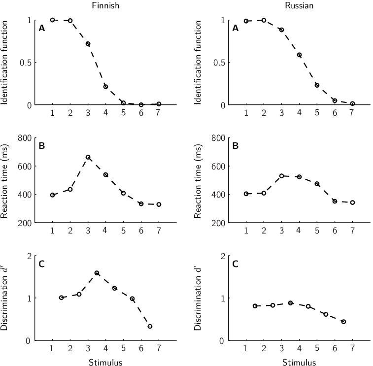
For a given stimulus $x$, the mean reaction time $\overline{\tau}(x)$ to categorize it is equal to the sum of the mean time $\tau_{nd}$ resulting from neural propagation and motor realization (independently of the decision), and the mean time $\overline{\tau_{d}}(x)$ characterizing the decision stage:

The mean time $\overline{\tau_{d}}(x)$ is given by formula (3.46) (using $\Phi_{a}$ here), and depends on three free variables: $F_{\text{code}}^{0}(x)$, $x_{f}$, and $\beta$. We first determine the Fisher information rate $F_{\text{code}}^{0}(x)$ thanks to experimental measures of $d^{\prime}$ and corresponding mean reaction times (measured during the discrimination task). The Fisher information rate $F_{\text{code}}^{0}(x)$ is linked to the perceptual distance $d^{\prime}$ through (Seung and Sompolinsky,, 1993, see e.g.):

where, here, $\delta x=1$. Moreover, as we have seen

where $\overline{\tau_{d}}^{\text{discrim}}(x)$ corresponds to the mean reaction times during the discrimination task. For a given stimulus $x$, we compute the quantity $\overline{\tau_{d}}^{\text{discrim}}(x)$ thanks to the mean reaction times measured by the authors, equal to $\overline{\tau_{RT}}^{\text{discrim}}(x)=\overline{\tau_{nd}}^{\text{discrim}}+\overline{\tau_{d}}^{\text{discrim}}(x)$, where $\overline{\tau_{nd}}^{\text{discrim}}$, the mean time resulting from neural propagation and motor realization, is independent of the decision, and is set to $250$ms. Applying a piecewise cubic Hermite interpolation to the experimentally measured values, we obtain an estimation of $d^{\prime}$ and of $\overline{\tau_{RT}}^{\text{discrim}}(x)$, and thus of $F_{\text{code}}^{0}(x)$, for all $x$ in the continuum.

Only three parameters are thus to be found in order to model the experimental data: $\tau_{nd}$, $x_{f}$ and $\beta$. For each group, these parameters are finally obtained by minimizing the least square error between experimental and predicted values. For the native speakers of Finnish, we get $\tau_{nd}^{\text{fin}}=280$, $\beta^{\text{fin}}=339$ and $x_{f}^{\text{fin}}=3.11$ (r=0.996, p=1.7e-6), and for the Russian group, $\tau_{nd}^{\text{rus}}=278$, $\beta^{\text{rus}}=463$ and $x_{f}^{\text{rus}}=3.85$ (r=0.959, p=6.5e-4). Figure 7 compares mean reaction times experimentally obtained with the ones predicted by formula (3.46), optimized for each case. In the case of native speakers of Finnish (Figure 7 (Left)), alignment between experimental data and prediction is almost perfect. In the case of the Russian group (Figure 7 (Right)), experimental data and predicted values line up remarkably well too.
Interestingly, the value of $\beta$ is found to be greater for the native speakers than for the non-native speakers. This parameter is equal to the ratio between $\gamma$, which is the decision threshold, and $b_{0}$, which quantifies the separation between the two categories. Thus, assuming one of the other parameter constant between groups, $\beta^{\text{fin}}<\beta^{\text{rus}}$ means that either the threshold is lower for the native speakers of Finnish than for the Russian group, or that the categories are more distinct for the natives. Both possibilities make sense here, given that we expect the native speakers to have a more accurate representation of the categories than the non-native speakers (the vocalic contrast used in this experiment being phonemic for the former group, but not for the latter).

It is worth noticing that only three free parameters are used here, thanks to the complete characterization of the $F_{\text{code}}^{0}(x)$ quantity using discrimination measurements. Other models of categorization response times do not allow for such a characterization, and would thus require more parameters.

References

- Abbott and Dayan, (1999) Abbott, L. and Dayan, P. (1999). The effect of correlated variability on the accuracy of a population code. Neural Comput., 11:91–101.
- Abramson and Lisker, (1970) Abramson, A. and Lisker, L. (1970). Discriminability along the voicing continuum: Cross-language tests. In Proc. of the VIth ICPhS Prague. Academia.
- Ashby, (2000) Ashby, F. (2000). A stochastic version of general recognition theory. J of Math Psychol, 44:310–329.
- Ashby and Maddox, (1993) Ashby, F. and Maddox, W. (1993). Relations between prototype, exemplar, and decision bound models of categorization. J of Math Psychol, 37:372–400.
- Ashby and Maddox, (1994) Ashby, F. and Maddox, W. (1994). A response time theory of separability and integrality in speeded classification. J of Math Psychol, 38:423–466.
- Ashby et al., (2007) Ashby, F. G., Ennis, J., and Spiering, B. J. (2007). A neurobiological theory of automaticity in perceptual categorization. Psychol Rev, 114(3):632–656.
- Beale and Keil, (1995) Beale, J. and Keil, F. (1995). Categorical effects in the perception of faces. Cognition, 57:217–239.
- Beck et al., (2008) Beck, J., Ma, W., Kiani, R., Hanks, T., Churchland, A., Roitman, J., Shadlen, M., Latham, P., and Pouget, A. (2008). Probabilistic population codes for bayesian decision making. Neuron, 60:1142–1152.
- Bialek et al., (2001) Bialek, W., Nemenman, I., and Tishby, N. (2001). Predictability, complexity, and learning. Neural Comput., 13:2409–2463.
- Bogacz and Gurney, (2007) Bogacz, R. and Gurney, K. (2007). The basal ganglia and cortex implement optimal decision making between alternative actions. Neural Comput., 19(2):442–477.
- Bonnasse-Gahot, (2009) Bonnasse-Gahot, L. (2009). Modélisation du codage neuronal de catégories et étude des conséquences perceptives. PhD thesis, École des Hautes Études en Sciences Sociales, Paris.
- Bonnasse-Gahot and Nadal, (2008) Bonnasse-Gahot, L. and Nadal, J.-P. (2008). Neural coding of categories: Information efficiency and optimal population codes. J. Comput. Neurosci., 25(1):169–87.
- Bornstein and Korda, (1984) Bornstein, M. and Korda, N. (1984). Discrimination and matching within and between hues measured by reaction times: some implications for categorical perception and levels of information processing. Psychol. Res., 46:207–222.
- Britten et al., (1992) Britten, K., Shadlen, M., Newsome, W., and Movshon, J. (1992). The analysis of visual motion: A comparison of neuronal and psychophysical performance. The Journal of Neuroscience, 12:4745–4765.
- Brunel and Nadal, (1998) Brunel, N. and Nadal, J.-P. (1998). Mutual information, fisher information, and population coding. Neural Comput., 10:1731–1757.
- Clarke and Barron, (1990) Clarke, B. and Barron, A. (1990). Information-theoretic asymptotics of bayes methods. IEEE Trans on Information Theory, 36(3):453–471.
- Cover and Thomas, (2006) Cover, T. and Thomas, J. (2006). Elements of Information Theory. Wiley & Sons, NY, USA. Second Edition.
- De Baene et al., (2008) De Baene, W., Ons, B., Wagemans, J., and Vogels, R. (2008). Effects of category learning on the stimulus selectivity of macaque inferior temporal neurons. Learn. Mem., 15:717–727.
- Duda et al., (2001) Duda, R., Hart, P., and Stork, D. (2001). Pattern Classification. Wiley, New York, USA. 2nd Edition.
- Ecker et al., (2010) Ecker, A., Berens, P., Keliris, G., Bethge, M., Logothetis, N., and Tolias, A. (2010). Decorrelated neuronal firing in cortical microcircuits. Science, 327:584–587.
- Freedman et al., (2001) Freedman, D., Riesenhuber, M., Poggio, T., and Miller, E. (2001). Categorical representation of visual stimuli in the primate prefrontal cortex. Science, 291:312–316.
- Freedman et al., (2002) Freedman, D., Riesenhuber, M., Poggio, T., and Miller, E. (2002). Visual categorization and the primate prefrontal cortex: Neurophysiology and behavior. J. Neurophysiol., 88:929–941.
- Freedman et al., (2003) Freedman, D., Riesenhuber, M., Poggio, T., and Miller, E. (2003). A comparison of primate prefrontal and inferior temporal cortices during visual categorization. J. Neurosci., 15:5235–5246.
- Gold and Shadlen, (2007) Gold, J. and Shadlen, M. (2007). The neural basis of decision making. Annu. Rev. Neurosci., 30:535–74.
- Goldstone, (1994) Goldstone, R. (1994). Influences of categorization on perceptual discrimination. J. Exp. Psychol. Gen., 123(2):178–200.
- Hallé et al., (2004) Hallé, P., Chang, Y.-C., and Best, C. (2004). Identification and discrimination of mandarin chinese tones by mandarin chinese vs. french listeners. J. Phonetics, 32:395–421.
- Harnad, (1987) Harnad, S., editor (1987). Categorical Perception: The Groundwork of Cognition. New York: Cambridge University Press.
- Haussler and Opper, (1995) Haussler, D. and Opper, M. (1995). General bounds on the mutual information between a parameter and n conditionally independent observations. Proc of the eighth ann conf on Computational Learning Theory, pages 402–41.
- Heekeren et al., (2004) Heekeren, H., Marret, S., Bandettini, P., and Ungerleider, L. (2004). A general mechanism for perceptual decision-making in the human brain. Nature, 431:859–862.
- Heeren and Schouten, (2008) Heeren, W. and Schouten, M. (2008). Perceptual development of phoneme contrasts: How sensitivity changes along acoustic dimensions that contrast phoneme categories. J. Acoust. Soc. Am., 124(4):2291–2302.
- Herschkowitz and Nadal, (1999) Herschkowitz, D. and Nadal, J.-P. (1999). Unsupervised and supervised learning: mutual information between parameters and observations. Phys. Rev. E, 59:3344–3360.
- Huk and Shadlen, (2005) Huk, A. and Shadlen, M. (2005). Neural activity in macaque parietal cortex reflects temporal integration of visual motion signals during perceptual decision making. J. Neurosci., 25(45):10420–10436.
- Kim and Shadlen, (1999) Kim, J. and Shadlen, M. (1999). Neural correlates of a decision in the dorsolateral prefrontal cortex of the macaque. Nat. Neurosci., 2(2):176–185.
- Kriegeskorte et al., (2008) Kriegeskorte, N., Mur, M., Ruff, D., Kiani, R., Bodurka, J., Esteki, H., Tanaka, K., and Bandettini, P. (2008). Matching categorical object representations in inferior temporal cortex of man and monkey. Neuron, 60:1126–1141.
- Kruschke, (1992) Kruschke, J. (1992). Alcove : An exemplar-based connectionist model of category learning. Psychol. Rev., 99(1):22–44.
- Kuhl, (2004) Kuhl, P. (2004). Early language acquisition : cracking the speech code. Nat. Rev. Neurosci., 5:831–843.
- Kuhl and Padden, (1983) Kuhl, P. and Padden, D. (1983). Enhanced discriminability at the phonetic boundaries for the place feature in macaques. J. Acoust. Soc. Am., 73(3):1003–1010.
- Kuhl et al., (1992) Kuhl, P., Williams, K., Lacerda, F., Stevens, K., and Lindblom, B. (1992). Linguistic experience alters phonetic perception in infants by 6 months of age. Science, 255:606–608.
- Liberman et al., (1957) Liberman, A., Harris, K., Hoffman, H., and Griffith, B. (1957). The discrimination of speech sounds within and across phoneme boundaries. J. Exp. Psychol., 54:358–369.
- Link, (1992) Link, S. (1992). The Wave Theory of Difference and Similarity. Lawrence Erlbaum Associates, Hillsdale, NJ.
- Link and Heath, (1975) Link, S. and Heath, R. (1975). A sequential theory of psychological discrimination. Psychometrika, 40(1):77–105.
- McMurray and Spivey, (2000) McMurray, B. and Spivey, M. (2000). The categorical perception of consonants: The interaction of learning and processing. Proc of the Chicago Linguistics Society, 34(2):205–220.
- Meyers et al., (2008) Meyers, E., Freedman, D., Kreiman, G., Miller, E., and Poggio, T. (2008). Dynamic population coding of category information in inferior temporal and prefrontal cortex. J. Neurophysiol., 100:1407–1419.
- Nosofsky, (1986) Nosofsky, R. (1986). Attention, similarity, and the identification-categorization relationship. J. Exp. Psychol., 115(1):39–57.
- Ohl et al., (2001) Ohl, F., Scheich, H., and Freeman, W. (2001). Change in pattern of ongoing cortical activity with auditory category learning. Nature, 412:733–736.
- Op de Beeck et al., (2008) Op de Beeck, H., Wagemans, J., and Vogels, R. (2008). The representation of perceived shape similarity and its role for category learning in monkeys: A modeling study. Vision Res., 48:598–610.
- Pisoni and Tash, (1974) Pisoni, D. and Tash, J. (1974). Reaction times to comparisons within and across phonetic categories. Percept. Psychophys., 15(2):285–290.
- Polka and Werker, (1994) Polka, L. and Werker, J. (1994). Developmental changes in perception of nonnative vowel contrasts. J. Exp. Psychol. Hum. Percept. Perf., 20(2):421–435.
- Prather et al., (2009) Prather, J., Nowicki, S., Anderson, R., Peters, S., and Mooney, R. (2009). Neural correlates of categorical perception in learned vocal communication. Nat. Neurosci., 12(2):221–228.
- Ratcliff, (1978) Ratcliff, R. (1978). A theory of memory retrieval. Psychol. Rev., 85:59–108.
- Ratcliff et al., (1999) Ratcliff, R., Van Zandt, T., and McKoon, G. (1999). Connectionist and diffusion models of reaction time. Psychol. Rev., 106(2):261–300.
- Renart et al., (2010) Renart, A., de la Rocha, J., Bartho, P., Hollender, L., Parga, N., Reyes, A., and Harris, K. (2010). The asynchronous state in cortical circuits. Science, 327:587–590.
- Repp, (1984) Repp, B. (1984). Categorical perception: issues, methods, findings. In Speech and Language: Advances in Basic Research and Practice.
- Rissanen, (1996) Rissanen, J. (1996). Fisher information and stochastic complexity. IEEE Trans. on Information Theory, 42(1):40–47.
- Rumelhart et al., (1986) Rumelhart, D., Hinton, G., and Williams, R. (1986). Learning representations by back-propagating errors. Nature, 323:533–536.
- Salinas and Romo, (1998) Salinas, E. and Romo, R. (1998). Conversion of sensory signals into motor commands in primary motor cortex. J. Neurosci., 18:499–511.
- Seung and Sompolinsky, (1993) Seung, H. S. and Sompolinsky, H. (1993). Simple models for reading neuronal population codes. PNAS, 90:10749–10753.
- Shadlen et al., (2006) Shadlen, M., Hanks, T., Churchland, A., Kiani, R., and Yang, T. (2006). The speed and accuracy of a simple perceptual decision: a mathematical primer. In Doya, K., Ishii, S., Rao, R., and Pouget, A., editors, Bayesian Brain: Probabilistc Approaches to Neural Coding, Cambridge, NY, USA. MIT Press.
- Shadlen and Newsome, (2001) Shadlen, M. and Newsome, W. (2001). Neural basis of a perceptual decision in the parietal cortex (area lip) of the rhesus monkey. J. Neurophysiol., 86:1916–1936.
- Sigala and Logothetis, (2002) Sigala, N. and Logothetis, N. (2002). Visual categorization shapes feature selectivity in the primate temporal cortex. Nature, 415:318–320.
- Smith and Ratcliff, (2004) Smith, P. and Ratcliff, R. (2004). Psychology and neurobiology of simple decisions. TINS, 27(3):161–167.
- Studdert-Kennedy et al., (1963) Studdert-Kennedy, M., Liberman, A., and Stevens, K. (1963). Reaction time to synthetic stop consonants and vowels at phoneme centers and at phoneme boundaries. J. Acoust. Soc. Am., 35(11):1900.
- Usher and McClelland, (2001) Usher, M. and McClelland, J. (2001). The time course of perceptual choice: The leaky, competing accumulator model. Psychol. Rev., 108(3):550–592.
- Vickers, (1970) Vickers, D. (1970). Evidence for an accumulator model of psychophysical discrimination. Ergonomics, 13:37–58.
- Wald, (1947) Wald, A. (1947). Sequential Analysis. Wiley, New York.
- Werker and Tees, (1984) Werker, J. and Tees, R. (1984). Cross-language speech perception: evidence for perceptual reorganization during the first year of life. Infant Behavior and Development, 7:49–63.
- Xu et al., (2006) Xu, Y., Gandour, J., and Francis, A. (2006). Effects of language experience and stimulus complexity on the categorical perception of pitch direction. J. Acoust. Soc. Am., 120:1063–1074.
- Ylinen et al., (2005) Ylinen, S., Shestakova, A., Alku, P., and Huotilainen, M. (2005). The perception of phonological quantity based on durational cues by native speakers, second-language users and nonspeakers of finnish. Lang. Speech, 48:313–338.
- Yoon and Sompolinsky, (1999) Yoon, H. and Sompolinsky, H. (1999). The effect of correlations on the fisher information of population codes. In Kearns, M., Solla, S., and Cohn, D., editors, Advances in neural information processing systems 11 (NIPS-11), pages 167–173. The MIT Press.
- Zohary et al., (1994) Zohary, E., Shadlen, M., and Newsome, W. (1994). Correlated neuronal discharge rate and its implications for psychophysical performance. Nature, 370:140–143.