Recursion Relations for AdS/CFT Correlators

Preprint: HRI/ST/1103

Suvrat Raju Affiliation: Harish-Chandra Research Institute, Affiliation: Jhunsi, Allahabad 211019. Email: suvrat@hri.res.in Affiliation: E-mail:

Abstract:

We expand on the results of arXiv:1011.0780 where we presented new recursion relations for correlation functions of the stress tensor and conserved currents in conformal field theories with an $\text{AdS}_{d+1}$ dual for $d\geq 4$ . These recursion relations are derived by generalizing the Britto-Cachazo-Feng-Witten (BCFW) relations to amplitudes in anti-de Sitter space (AdS) that are dual to boundary correlators, and are usually computed perturbatively by Witten diagrams. Our results relate vacuum-correlation functions to integrated products of lower-point transition amplitudes, which correspond to correlators calculated between states dual to certain normalizable modes. We show that the set of “polarization vectors” for which amplitudes behave well under the BCFW extension is smaller than in flat-space. We describe how transition amplitudes for more general external polarizations can be constructed by combining answers obtained by different pairs of BCFW shifts. We then generalize these recursion relations to supersymmetric theories. In AdS, unlike flat-space, even maximal supersymmetry is insufficient to permit the computation of all correlators of operators in the same multiplet as a stress-tensor or conserved current. Finally, we work out some simple examples to verify our results.

Keywords:

AdS/CFT, correlation functions, BCFW recursion relations, S-matrix

1 Introduction

The Britto-Cachazo-Feng-Witten (BCFW) recursion relations [1, 2] have attracted interest because they provide a novel way of calculating S-matrix elements in gauge and gravity theories. These relations reproduce the answers provided by standard Feynman-diagram perturbation theory but are far more efficient. This provides an immediate practical motivation for these investigations: the study of scattering amplitudes that are of phenomenological relevance at particle accelerators. Indeed, using the BCFW relations and associated on-shell techniques at one loop [3] – [10], Berger et al. [11] were able to calculate the next-to-leading order correction for the production of W + 4-jets at the Large Hadron Collider (LHC) — a calculation that had remained out of the reach of conventional Feynman diagram techniques. Earlier, two groups used similar techniques to understand the production of W + 3-jets at both the Tevatron and the LHC [12, 13, 14].

Another example, which is relevant to quantum gravity, comes from scattering amplitudes of gravitons. If the Hilbert action is expanded in metric fluctuations, one obtains an infinite series of interaction vertices of ever increasing complexity; for example, the four-point vertex already has 2850 terms! However, the interactions of gravitons are not really that complicated: the final answers for scattering amplitudes are quite simple. In fact, DeWitt who first worked out scattering amplitudes for gravitons commented that “the tediousness of the algebra involved …combined with the fact that the final results are ridiculously simple, leads one to believe that there must be an easier way.”[15] The BCFW recursion relations are this “easier way”! They reduce the computation of all graviton scattering amplitudes down to the computation of the on-shell three-point function, which is completely determined by Lorentz invariance.

This leads us to a second, more fundamental, reason for the interest in the BCFW relations. Since the BCFW recursion relations are ostensibly so different from Feynman diagrams but, yet, provide a shortcut to the final answer, we would like to find a formulation of quantum field theory (QFT) in which these recursion relations, rather than Feynman diagrams, are the “natural” objects of study. A new such formulation of QFT, if it were to be discovered, would certainly be important for our understanding of basic physics.

The search for such a formulation has attracted much recent interest. An important attempt was made by Witten [16] who tried to formulate gauge theory as a string theory in twistor space. Although this did not succeed entirely it led to the discovery of the BCFW recursion relations. More-recent work that has aimed at uncovering the underlying physics in these relations includes a reformulation of the BCFW relations in twistor space [17, 18] and the attempt to find a Grassmannian integral [19, 20] which would produce the leading singularities of scattering amplitudes at all loops and the BCFW recursion relations at tree-level. For other recent extensions to higher-loops we refer the reader to [21, 22].

This programme of reformulating quantum field theory is ambitious but has not yet succeeded. Nevertheless, it is clear that the secret of the efficiency of the BCFW recursion relations, and on-shell techniques in general, is that they make reference only to the physical degrees of freedom in a theory. On the other hand, this comes at the price of manifest locality. In a rough sense, this is analogous to the way in which the path-integral formulation of QFT makes Lorentz-invariance manifest but obscures unitarity; the Hamiltonian formulation, on the other hand, makes unitarity manifest but obscures Lorentz-invariance. The on-shell formulation that we are looking for would make the simplicity of amplitudes and physical degrees of freedom manifest but perhaps obscure locality.

All the studies that we have referred to above were carried out in flat-space. In fact, until recently, it was believed that on-shell techniques apply only to quantum field theories in flat-space. This is because they rely heavily on the analytic properties of amplitudes, which change drastically in curved spacetime. In a recent letter [23] we pointed out that the BCFW recursion relations could be generalized to gauge and gravity theories in anti-de Sitter space (AdS). By the AdS/CFT correspondence, this gives new and surprising recursion relations for correlators in the boundary conformal field theory (CFT).

The physical intuition underlying this surprising result is as follows. The BCFW recursion relations are predicated on the behaviour of Yang-Mills (YM) and gravity amplitudes when two of the external momenta are stretched off the infinity in a “complex direction.” Although this is not strictly a high energy limit, it is nonetheless true that the amplitude is dominated by interactions between a soft background and a highly boosted particle at a single point [24]. In this limit, we do not expect this highly boosted particle to see the curvature of the neighboring spacetime region. Viewed from this perspective, the properties of an amplitude under the BCFW extension should not change much as we go from flat-space to curved space, except for one crucial difference: in flat-space, the location of this interaction-point does not matter whereas in curved space it does. So, in AdS we need to integrate over the different points where this interaction can occur. (This is similar to the intuition used in [25].) This process leads to the modified recursion relations that we present below. A higher-point correlator is broken down into the integral of the product of two lower-point correlators. Just as in flat-space, we can continue this process till we are left only with three-point functions.

Once again, this is of interest for two reasons. First, the inordinate complexity of gravity is exacerbated when we expand metric fluctuations about AdS. As a result, even the smallest nontrivial correlators, like the four-point function of the stress-tensor in strongly coupled ${{\mathcal{N}}=4}$ Super-Yang-Mills theory (SYM) that is dual to the scattering of four-gravitons in the bulk, have never been computed directly.¹¹ 1 This correlator may, in principle, be extracted from simpler correlators using superconformal invariance [26, 27] but this has never been done explicitly either. On the other hand, as far as know, its direct computation using Witten diagrams has not even been attempted. Correlators of the stress-tensor are of particular interest because their leading behaviour is “universal” in any conformal field theory with a gravity dual due to the fact that tree-level graviton amplitudes are not sensitive to the matter-content of the theory. Since, as in flat-space, the repeated application of our recursion relations allows us to reduce complicated amplitudes down to three-point functions, we expect that our new recursion relations will greatly simplify the computation of these correlators. On the other hand, as we discuss in more detail in section 7, these relations are also of interest for formal reasons — both for what they teach us about quantum gravity in asymptotically anti-de Sitter spaces and for what they teach us about conformal field theories with a gravity dual.

Finally, we should mention one interesting feature of our results. If we set out to compute a vacuum-correlator in the boundary theory, with all normalizable modes switched off in the bulk, the recursion relations lead us to correlators computed in the presence of specific states; in the bulk, this corresponds to turning on some normalizable modes. We will call these generalized correlators “transition amplitudes.”

These transition amplitudes have a nice physical interpretation in Lorentzian AdS. There has been much recent discussion of the subtleties associated with Lorentzian AdS/ CFT; these subtleties are not too important here especially since we are are at zero temperature. However, the reader who is concerned about this may instead prefer to work all the time in the Euclidean picture and only analytically continue the results at the end. In the Euclidean picture, the intermediate objects that we obtain in our recursion relations do not have any direct physical interpretation (except as the analytic continuation of Lorentzian transition amplitudes) but they are well defined formal quantities that one can compute in perturbation theory.

A brief overview of this paper is as follows. We start with a review of perturbation theory in AdS in section 2. We then proceed to define and discuss transition amplitudes in section 3. The central results in the paper are derived in section 4 where we derive new recursion relations for transition amplitudes in Yang-Mills theory and gravity.

A further extension of our recursion relations in section 5 allows us to compute transition amplitudes in supersymmetric theories, including ${{\mathcal{N}}=4}$ SYM and the theory on multiple M5 branes in the supergravity limit. Perturbative computations in supersymmetric theories are often tedious; the recursion relations that we present ameliorate this by using a generalization of Nair’s on-shell superspace [28]. We would suggest that the reader, who is interested just in the results of this paper, should read [23] first and then turn here for details.

2 Review of Perturbation Theory

We will work in Poincare coordinates where the metric is

ds^{2}=g_{\mu\nu}dx^{\mu}dx^{\nu}=z^{-2}\left(dz^{2}+\eta_{ij}dx^{i}dx^{j}\right).

(1)

Note that we are using the mostly positive signature for the boundary metric. Poincare invariance in $d$ -dimensions makes it convenient to Fourier transform functions of $x^{i}$ and we will call the conjugate variables — $k_{i}$ — “momenta.”These are really momenta in the dual conformal field theory. Note that we will use boldface for tensors and vectors in $d$ or $d+1$ dimensions, like ${\boldsymbol{x}}$ or ${\boldsymbol{k}}$ , but not for their components. While considering momenta in a $n$ -particle amplitude, we will often use the index $m$ to run over the various particles from $1$ to $n$ ; these have momenta from ${\boldsymbol{k_{1}}}$ to ${\boldsymbol{k_{n}}}$ . At times, to lighten the notation, especially when we are dealing with “polarization vectors”, ${\boldsymbol{\epsilon_{m}}}$ , below we might raise the particle-number index i.e. write ${\boldsymbol{\epsilon^{m}}}$ instead; this does not have any significance.

The indices, $i,j$ are reserved for the $d$ -dimensional spacetime coordinates. We will avoid raising and lowering these indices; for example $x^{i}$ naturally has a raised index, while $k_{i}$ or a gauge field $A_{i}^{\rm a}$ naturally has lowered indices. However, when we need to take a dot product of two $d$ -dimensional vectors, we will use the flat-space metric. On the other hand, $\mu,\nu$ run over all $d+1$ dimensions. When we raise or lower one of these indices, we will use the full metric including the factors of $z$ . Finally, the index $0$ will refer to the $z$ -direction while the boundary coordinates run from $1\ldots d.$

Perturbation theory in AdS is carried out through Witten diagrams. This requires two crucial ingredients: the bulk to boundary propagator, and the bulk to bulk propagator. The bulk to boundary propagator is a certain kind of solution to the equations of motion — called a non-normalizable solution — with some special boundary conditions. We discuss these two physical quantities for scalars, gauge fields and gravity below. These results are well known but, at times, such as in the expression for the gauge and gravity propagators, we were unable to find them in the literature in the exact-form that we required. So, we have tried to be as detailed as possible.

2.1 Scalars

We start by describing solutions to the wave equation and then go on to describe propagators in AdS.

2.1.1 Solutions to the Wave Equation

Consider a minimally coupled massless scalar. Its equation of motion is

\Box\phi=0\Rightarrow\partial_{\mu}g^{\mu\nu}\sqrt{-g}\partial_{\nu}\phi=0.

(2)

Poincare invariance in $d$ -dimensions tells us that all solutions can be written as linear combinations of $\phi_{{\boldsymbol{k}}}({\boldsymbol{x}},z)=e^{i{\boldsymbol{k}}\cdot{\boldsymbol{x}}}\phi(z)$ where $\phi_{{\boldsymbol{k}}}$ satisfies

\bigl(\partial_{z}z^{1-d}\partial_{z}-z^{1-d}{\boldsymbol{k}}^{2}\bigr)\phi_{{\boldsymbol{k}}}=0.

(3)

Here, ${\boldsymbol{k}}^{2}=\eta^{ij}k_{i}k_{j}$ is taken with the flat boundary metric. If ${\boldsymbol{k}}$ is timelike, which means ${\boldsymbol{k}}^{2}<0$ , then there are two solutions to (3)

\begin{split}\text{normalizable:}\quad&\phi(z)=z^{\nu}\phi_{0}J_{\nu}(|{\boldsymbol{k}}|z),\\ \text{non-normalizable:}\quad&\phi(z)=z^{\nu}\phi_{0}Y_{\nu}(|{\boldsymbol{k}}|z),\end{split}

(4)

where $J_{\nu}$ and $Y_{\nu}$ are Bessel functions of the first and second kind respectively. Moreover, $|{\boldsymbol{k}}|=\sqrt{|{\boldsymbol{k}}^{2}|}$ , $\nu={d\over 2}$ and²² 2 We hope this notation will not cause confusion with the use of $\nu$ as a spacetime index. $\phi_{0}$ is some constant. Any linear combination of these solutions is also a solution to the equation of motion.

On the other hand, if ${\boldsymbol{k}}$ is spacelike then the requirement that the solution be regular in the interior of AdS fixes the solution to be

\phi(z)=z^{\nu}\phi_{0}K_{\nu}(|{\boldsymbol{k}}|z),\quad\text{for}~{\boldsymbol{k}}^{2}>0,

(5)

where $K$ is the modified Bessel function of the second kind.

Note that the analytic continuation of (5) to timelike momenta gives a solution involving the Hankel function of the first kind³³ 3 The factor of ${\pi\over 2}i^{\nu+1}$ is customary in the definition of the modified Bessel functions. We should also add here that we are not being very precise about the overall normalization of these solutions since this is not important for any part of the analysis in this paper

\phi(z)=z^{\nu}\phi_{0}{\pi\over 2}i^{\nu+1}H_{\nu}^{(1)}(|{\boldsymbol{k}}|z)=z^{\nu}\phi_{0}{\pi\over 2}i^{\nu+1}\left(J_{\nu}(|{\boldsymbol{k}}|z)+iY_{\nu}(|{\boldsymbol{k}}|z)\right),~\text{for}~{\boldsymbol{k}}^{2}<0.

(6)

If we are calculating time-ordered correlation functions on the boundary, then this is the correct bulk to boundary propagator [29, 30]. This is because, as we approach the Poincare horizon at $z=\infty$ , this bulk to boundary propagator ensures that positive energy waves are ingoing whereas negative energy waves are outgoing.

In some contexts, we will find that the distinction between these solutions is unimportant. We will then write $\phi_{{\boldsymbol{k}}}({\boldsymbol{x}},z)=\phi_{0}e^{i{\boldsymbol{k}}\cdot{\boldsymbol{x}}}E_{\nu}({\boldsymbol{k}},z)$ where $z^{-\nu}E_{\nu}({\boldsymbol{k}},z)$ is one of the Bessel functions, $K_{\nu}({\boldsymbol{k}}z),J_{\nu}({\boldsymbol{k}}z),Y_{\nu}({\boldsymbol{k}}z)$ , or a linear combination of these functions.

2.1.2 Propagator

We now turn to the bulk to bulk propagator. Here, we will just call this the propagator. The propagator is the Green’s function that satisfies (in $d+1$ dimensions),

\Box G({\boldsymbol{x}},z,{\boldsymbol{x^{\prime}}},z^{\prime})=i{\delta^{d}({\boldsymbol{x}}-{\boldsymbol{x^{\prime}}})\delta(z-z^{\prime})\over\sqrt{-g}}.

(7)

Note that the left hand side is invariant under coordinate transformations and the $\sqrt{-g}$ ensures that this is also true for the right hand side, because it cancels the transformation of the $\delta$ function. (See Eqn. (3.49) of [31].) Under a coordinate transformation with Jacobian $J$ , we have $\delta^{d}(x-x^{\prime})\delta(z-z^{\prime})\rightarrow\delta^{d}(x-x^{\prime})\delta(z-z^{\prime})/J$ and $\sqrt{-g}\rightarrow\sqrt{-g}/J$ . With the metric (1) we have $\sqrt{-g}={1\over z^{d+1}}$ .

After we Fourier transform from ${\boldsymbol{x}}$ to ${\boldsymbol{k}}$

G_{{\boldsymbol{k}}}(z,z^{\prime})=\int G({\boldsymbol{x}},z,{\boldsymbol{x^{\prime}}},z^{\prime})e^{-i{\boldsymbol{k}}\cdot({\boldsymbol{x}}-{\boldsymbol{x^{\prime}}})}d^{d}x,

(8)

the equation (7) becomes

z^{d+1}{\partial\over\partial z}z^{1-d}{\partial G_{{\boldsymbol{k}}}\over\partial z}-z^{2}{\boldsymbol{k}}^{2}G_{{\boldsymbol{k}}}=i\delta(z-z^{\prime})z^{d+1}.

(9)

Using the identity,

\int zJ_{\nu}(pz)J_{\nu}(p^{\prime}z)dz={\delta(p-p^{\prime})\over p},

(10)

we see that the solution to (9) is

G_{{\boldsymbol{k}}}(z,z^{\prime})=\int{-ip\,dp\over\left({\boldsymbol{k}}^{2}+p^{2}-i\epsilon\right)}z^{\nu}J_{\nu}(pz)J_{\nu}(pz^{\prime})(z^{\prime})^{\nu},

(11)

and, as usual,

\begin{split}G({\boldsymbol{x}},z,{\boldsymbol{x^{\prime}}},z^{\prime})&=\int{d^{d}{\boldsymbol{k}}\over(2\pi)^{d}}G_{{\boldsymbol{k}}}(z,z^{\prime})e^{i{\boldsymbol{k}}\cdot({\boldsymbol{x}}-{\boldsymbol{x^{\prime}}})}\\ &=\int{-id^{d}{\boldsymbol{k}}\over(2\pi)^{d}}{dp^{2}\over 2}{e^{i{\boldsymbol{k}}\cdot({\boldsymbol{x}}-{\boldsymbol{x^{\prime}}})}z^{\nu}J_{\nu}(pz)J_{\nu}(pz^{\prime})(z^{\prime})^{\nu}\over\left({\boldsymbol{k}}^{2}+p^{2}-i\epsilon\right)},\end{split}

(12)

We draw the attention of the reader to one property of the momentum space propagator which will be important to us below. When the denominator of its integrand goes on shell i.e. when $p^{2}=-{\boldsymbol{k}}^{2}$ , the numerator breaks up into a sum over a product of normalizable modes. This is the same as what happens in flat-space, and is expected because the propagator is just a two-point function.

2.2 Gauge Fields

We now turn to vector fields in AdS. These are dual to conserved currents on the boundary. Both the solutions to the equations of motion and the propagator depend on the choice of gauge. Here, we will choose axial gauge so that for the gauge field $A^{\rm a}_{\mu}$ in the bulk: $A^{\rm a}_{0}=0.$ Note that we do not italicize the color-index ${\rm a}$ .

The bulk action is

S={-1\over 4}\int\sqrt{-g}F_{\mu\nu}^{\rm a}F^{\mu\nu,\rm{a}}d^{d}{\boldsymbol{x}}dz.

(13)

To go to “axial gauge”, we add a gauge fixing term $\zeta\sum_{\rm a}(A^{\rm a}_{0})^{2}$ and take $\zeta\rightarrow-\infty$ . This freezes $A^{\rm a}_{0}=0$ . We also set the coupling constant, $g_{\text{YM}}=0$ for now, although we will turn it on later to examine interactions in this theory. With these choices, we have the gauge-fixed action

\begin{split}{S}_{\text{axial}}&={1\over 2}\int\left[A^{\rm a}_{i}\partial_{\mu}z^{3-d}\partial_{\rho}A^{\rm a}_{j}\eta^{\mu\rho}\eta^{ij}-z^{3-d}A^{\rm a}_{i}\partial_{k}\partial_{l}A^{\rm a}_{j}\eta^{ik}\eta^{jl}\right]d^{d}{\boldsymbol{x}}dz+S_{\text{axial}}^{\cal B}.\end{split}

(14)

Note that we have used the fact that $A_{0}^{\rm a}=0$ and also integrated by parts; $S_{\text{axial}}^{\cal B}$ is the resultant boundary term, which does not affect the equations of motion.

From (14), we can read off both the solutions to the free-equations of motion and the propagator. Solutions to the equations of motion,

A^{\rm a}_{i}({\boldsymbol{x}},z)=\int A^{\rm a}_{i}({\boldsymbol{k}},z)e^{+i{\boldsymbol{k}}\cdot{\boldsymbol{x}}}d^{d}{\boldsymbol{x}},

(15)

must satisfy

{\boldsymbol{k}}\cdot{\boldsymbol{A^{\rm a}}}({\boldsymbol{k}},z)=0,

(16)

in the gauge $A^{\rm a}_{0}({\boldsymbol{k}},z)=0$ and also

\partial_{0}z^{3-d}\partial_{0}A^{\rm a}_{i}-k^{2}z^{3-d}A^{\rm a}_{i}=0.

(17)

For timelike ${\boldsymbol{k}}$ , this has the two solutions

\begin{split}\text{normalizable:}\quad A^{\rm a}_{i}({\boldsymbol{k}},z)&=\epsilon_{i}^{\rm a}z^{\nu_{1}}J_{\nu_{1}}(|{\boldsymbol{k}}|z),\\ \text{non-normalizable:}\quad A^{\rm a}_{i}({\boldsymbol{k}},z)&=\epsilon_{i}^{\rm a}z^{\nu_{1}}Y_{\nu_{1}}(|{\boldsymbol{k}}|z).\end{split}

(18)

Here $\nu_{1}=\nu-1$ and the polarization vector ${\boldsymbol{\epsilon}}$ must satisfy

{\boldsymbol{k}}\cdot{\boldsymbol{\epsilon}}^{\rm a}=0.

(19)

The timelike bulk to boundary propagator is a linear combination of these solutions that has the correct boundary conditions at $z\rightarrow\infty$ :

A^{\rm a}_{i}({\boldsymbol{k}},z)=\epsilon_{i}^{\rm a}z^{\nu_{1}}H_{\nu_{1}}^{(1)}(|{\boldsymbol{k}}|z),~\text{for}~{\boldsymbol{k}}^{2}<0.

(20)

On the other hand, for spacelike ${\boldsymbol{k}}$ , we have the unique solution:

A^{\rm a}_{i}({\boldsymbol{k}},z)=\epsilon_{i}^{\rm a}z^{\nu_{1}}K_{\nu_{1}}(|{\boldsymbol{k}}|z),~\text{for}~{\boldsymbol{k}}^{2}<0.

(21)

This is also the bulk to boundary propagator for spacelike momentum and its analytic continuation to timelike momenta gives (20). Inverting the quadratic operator in (14) leads to the propagator:

\begin{split}&G^{\text{axial},{\rm ab}}_{ij}({\boldsymbol{x}},z,{\boldsymbol{x}}^{\prime},z^{\prime})=\int{-id^{d}{\boldsymbol{k}}dp^{2}\over 2(2\pi)^{d}}{e^{i{\boldsymbol{k}}\cdot({\boldsymbol{x}}-{\boldsymbol{x^{\prime}}})}}\Bigl[{(zz^{\prime})^{\nu_{1}}J_{\nu_{1}}(pz)J_{\nu_{1}}(pz^{\prime}){\cal T}_{ij}\delta^{ab}\over\left({\boldsymbol{k}}^{2}+p^{2}-i\epsilon\right)}\Bigr],\end{split}

(22)

where ${\cal T}_{ij}=\eta_{ij}+{k_{i}k_{j}\over p^{2}}$ Once again we emphasize that at ${\boldsymbol{k}}^{2}=-p^{2}$ , ${\cal T}_{ij}$ just projects vectors onto the space orthogonal to ${\boldsymbol{k}}$ and so the numerator of (22) breaks up into the sum over a product of normalizable modes.

Comparison with Liu-Tseytlin:

We pause to compare our propagator to the one given by Liu and Tseytlin [32]. Referring to Eqn. (4.6) of their paper (from version 4 on the arXiv), we see that, in the presence of a bulk-source ${\boldsymbol{T}}$ , we can write the quadratic action as

\begin{split}2S_{LT}&=\int{dzdz^{\prime}{\cal D}({\boldsymbol{k}},{\boldsymbol{x}},{\boldsymbol{x^{\prime}}})dp^{2}\over 2z^{d+1}(z^{\prime})^{d+1}}T^{i}(z)\left[{\eta_{ij}-{k_{i}k_{j}\over{\boldsymbol{k}}^{2}}\over{\boldsymbol{k}}^{2}+p^{2}}\right]T^{j}(z^{\prime})z^{\nu_{1}}J_{\nu_{1}}(|{\boldsymbol{k}}|z)(z^{\prime})^{\nu_{1}}J_{\nu_{1}}(|{\boldsymbol{k}}|z^{\prime})\\ &+\int T^{0}({\boldsymbol{x}},z)T^{0}({\boldsymbol{x^{\prime}}},z){1\over{\boldsymbol{k}}^{2}}{{\cal D}({\boldsymbol{k}},{\boldsymbol{x}},{\boldsymbol{x^{\prime}}})dz\over z^{d+5}}.\end{split}

(23)

Note that (a) we have adopted the notation

{\cal D}({\boldsymbol{k}},{\boldsymbol{x}},{\boldsymbol{x^{\prime}}})\equiv d^{d}{\boldsymbol{x}}d^{d}{\boldsymbol{x^{\prime}}}{d^{d}{\boldsymbol{k}}\over(2\pi)^{d}}e^{i{\boldsymbol{k}}\cdot({\boldsymbol{x}}-{\boldsymbol{x^{\prime}}})},

(24)

(b) we have raised indices for the currents, which we have denoted by ${\boldsymbol{T}}$ to avoid confusion with Bessel functions; this leads to slightly different factors of z. Moreover, we have only displayed the $z$ dependence in the source which may also depend on ${\boldsymbol{x}}$ . (c) We have a minus sign in the second term by virtue of having ${\boldsymbol{k}}^{2}$ rather than $\partial^{2}$ and (d) $\nu_{1}={d-2\over 2}$ . On the other hand, we also have

\begin{split}&2S_{\rm axial}=\int{dzdz^{\prime}{\cal D}({\boldsymbol{k}},{\boldsymbol{x}},{\boldsymbol{x^{\prime}}})dp^{2}\over 2z^{d+1}(z^{\prime})^{d+1}}T^{i}(z)\left[{\eta_{ij}+{k_{i}k_{j}\over p^{2}}\over{\boldsymbol{k}}^{2}+p^{2}}\right]T^{j}(z^{\prime})z^{\nu_{1}}J_{\nu_{1}}(|{\boldsymbol{k}}|z)(z^{\prime})^{\nu_{1}}J_{\nu_{1}}(|{\boldsymbol{k}}|z^{\prime}),\end{split}

(25)

so that

\begin{split}&2S_{LT}-2S_{\rm axial}\\ &=\int{dzdz^{\prime}{\cal D}({\boldsymbol{k}},{\boldsymbol{x}},{\boldsymbol{x^{\prime}}})dp^{2}\over 2z^{d+1}(z^{\prime})^{d+1}}T^{i}(z)\left[{{-k_{i}k_{j}\over k^{2}}-{k_{i}k_{j}\over p^{2}}\over k^{2}+p^{2}}\right]T^{j}(z^{\prime})z^{\nu_{1}}J_{\nu_{1}}(|{\boldsymbol{k}}|z)(z^{\prime})^{\nu_{1}}J_{\nu_{1}}(|{\boldsymbol{k}}|z^{\prime})\\ &+\int T^{0}(z)T^{0}(z){1\over{\boldsymbol{k}}^{2}}{{\cal D}({\boldsymbol{k}},{\boldsymbol{x}},{\boldsymbol{x^{\prime}}})dz\over z^{d+5}}\\ &=\int{dzdz^{\prime}{\cal D}({\boldsymbol{k}},{\boldsymbol{x}},{\boldsymbol{x^{\prime}}})dp^{2}\over 2z^{d+1}(z^{\prime})^{d+1}}T^{i}(z)\left[{-k_{i}k_{j}\over{\boldsymbol{k}}^{2}p^{2}}\right]T^{j}(z^{\prime})z^{\nu_{1}}J_{\nu_{1}}(|{\boldsymbol{k}}|z)(z^{\prime})^{\nu_{1}}J_{\nu_{1}}({\boldsymbol{x^{\prime}}},z^{\prime})\\ &+\int T^{0}(z)T^{0}(z){1\over{\boldsymbol{k}}^{2}}{{\cal D}({\boldsymbol{k}},{\boldsymbol{x}},{\boldsymbol{x^{\prime}}})dz\over z^{d+5}}.\end{split}

(26)

We now use the identities

\begin{split}&\int_{0}^{\infty}J_{\nu_{1}}(pz)J_{\nu_{1}}(pz^{\prime}){dp\over p}={\theta(z-z^{\prime})\over 2\nu_{1}}\left({z^{\prime}\over z}\right)^{\nu_{1}}+{\theta(z^{\prime}-z)\over 2\nu_{1}}\left({z\over z^{\prime}}\right)^{\nu},\\ &\partial_{i}T^{i}=-{1\over\sqrt{-g}}\partial_{0}\sqrt{-g}T^{0},\end{split}

(27)

where the second line comes from current conservation and is useful because we can replace $k_{i}k_{j}\rightarrow\partial_{i}\partial_{j}^{\prime}$ . Note that one derivative pulls down an $i$ and the other pulls down a $(-i)$ , so there is no overall minus sign. Substituting this into the equation above, and integrating by parts, we see that

\begin{split}&2(S_{LT}-S_{\rm axial})\\ &=-\int{dzdz^{\prime}{\cal D}({\boldsymbol{k}},{\boldsymbol{x}},{\boldsymbol{x^{\prime}}})\over z^{d+1}(z^{\prime})^{d+1}}{1\over k^{2}}T^{0}(z)T^{0}(z^{\prime}){\cal P}_{\theta,z,z^{\prime}}+\int T^{0}(z)T^{0}(z){{\cal D}({\boldsymbol{k}},{\boldsymbol{x}},{\boldsymbol{x^{\prime}}})\over k^{2}}{dz\over z^{d+5}}.\end{split}

(28)

where we have defined

{\cal P}_{\theta,z,z^{\prime}}\equiv{\partial^{2}\over\partial z\partial z^{\prime}}\left({z^{\nu_{1}}(z^{\prime})^{\nu_{1}}\over 2\nu_{1}}\left[\theta(z-z^{\prime})\left({z^{\prime}\over z}\right)^{\nu_{1}}+\theta(z^{\prime}-z)\left({z\over z^{\prime}}\right)^{\nu_{1}}\right]\right).

(29)

Carefully working out the derivative, we find

\begin{split}{\cal P}_{\theta,z,z^{\prime}}&={\partial\over\partial z^{\prime}}\left[{\partial\over\partial z}\left((z^{\prime})^{2\nu_{1}}\theta(z-z^{\prime})+z^{2\nu_{1}}\theta(z^{\prime}-z)\right)\right]\\ &={\partial\over\partial z^{\prime}}\left[(z^{\prime})^{2\nu_{1}}\delta(z-z^{\prime})-z^{2\nu_{1}}\delta(z^{\prime}-z)+{2\nu_{1}}z^{2\nu_{1}-1}\theta(z^{\prime}-z)\right]\\ &={\partial\over\partial z^{\prime}}{2\nu_{1}}z^{2\nu_{1}-1}\theta(z^{\prime}-z)=2\nu_{1}z^{2\nu_{1}-1}\delta(z^{\prime}-z).\end{split}

(30)

Substituting this into (28), we see that everything cancels out miraculously and we get

S_{LT}-S_{\rm axial}=0.

(31)

So, our propagator is the same as the propagator given by Liu and Tseytlin although the two are written in slightly different forms.

2.3 Gravity

Now, we turn to gravitons propagating in AdS. We expand gravity fluctuations about a background metric ${\mathcal{G}}_{\mu\nu}=g_{\mu\nu}+h_{\mu\nu}$ , where $g_{\mu\nu}$ is the background and $h_{\mu\nu}$ contains the fluctuations. We can take the quadratic gravity action from [33]. As in the subsection above, boundary terms affect neither the equations of motion nor the propagator, so we will neglect them here. The quadratic action is given by

S={-1\over 64\pi G}\int{d^{d}{\boldsymbol{x}}dz\over z^{d+1}}\left(\tilde{h}^{\mu\nu}\Box h_{\mu\nu}+2\tilde{h}^{\mu\nu}R_{\mu\rho\nu\sigma}h^{\rho\sigma}+2\nabla^{\rho}\tilde{h}_{\rho\mu}\nabla^{\sigma}\tilde{h}_{\sigma}^{\mu}\right),

(32)

where $\tilde{h}^{\mu\nu}=h^{\mu\nu}-{1\over 2}g^{\mu\nu}h^{\alpha\beta}g_{\alpha\beta}$ , and all covariant derivatives are with respect to the background metric.

We want to analyze this action, when the background metric is the AdS metric, in axial gauge $h_{\mu 0}=0.$ Before we parse this action, let us write down a few simple identities. The connection coefficients are given by

\Gamma^{\rho}_{\alpha\beta}={1\over 2}g^{\rho\delta}\left(\partial_{\alpha}g_{\beta\delta}+\partial_{\beta}g_{\alpha\delta}-\partial_{\delta}g_{\alpha\beta}\right)={1\over z}\left(\delta^{\rho}_{0}\eta_{\alpha\beta}-\delta^{0}_{\alpha}\delta^{\rho}_{\beta}-\delta^{0}_{\beta}\delta^{\rho}_{\alpha}\right),

(33)

Using these coefficients, we see that

\begin{split}\nabla_{\rho}h_{\mu\nu}&=\partial_{\rho}h_{\mu\nu}-\Gamma^{\alpha}_{\rho\mu}h_{\alpha\nu}-\Gamma^{\alpha}_{\rho\nu}h_{\mu\alpha}\\ &=\partial_{\rho}h_{\mu\nu}+{1\over z}\left(2\delta^{0}_{\rho}h_{\mu\nu}+\delta^{0}_{\mu}h_{\rho\nu}+\delta^{0}_{\nu}h_{\mu\rho}\right)\\ &={1\over z^{2}}\left(\partial_{\rho}(z^{2}h_{\mu\nu})+z\delta^{0}_{\mu}h_{\rho\nu}+z\delta^{0}_{\nu}h_{\mu\rho}\right).\end{split}

(34)

In particular, in the action, we have a term of the kind

\begin{split}&\sqrt{-g}g^{\gamma\rho}g^{\mu\mu_{1}}g^{\nu\nu_{1}}\nabla_{\gamma}h_{\mu_{1}\nu_{1}}\nabla_{\rho}h_{\mu\nu}\\ &=z^{1-d}\eta^{\gamma\rho}\eta^{\mu\mu_{1}}\eta^{\nu\nu_{1}}\left[\partial_{\gamma}(z^{2}h_{\mu_{1}\nu_{1}})+z\delta^{0}_{\mu_{1}}h_{\gamma\nu_{1}}+z\delta^{0}_{\nu_{1}}h_{\mu_{1}\gamma}\right]\left[\partial_{\rho}(z^{2}h_{\mu\nu})+\delta^{0}_{\mu}zh_{\rho\nu}+z\delta^{0}_{\nu}h_{\mu\rho}\right].\end{split}

(35)

Note that when we expand this product out, the cross-terms all contract to zero with our choice of gauge. However, we are left with

\sqrt{-g}g^{\gamma\rho}g^{\mu\mu_{1}}g^{\nu\nu_{1}}\nabla_{\gamma}h_{\mu_{1}\nu_{1}}\nabla_{\rho}h_{\mu\nu}=z^{1-d}\eta^{\mu\mu_{1}}\eta^{\nu\nu_{1}}\left[\eta^{\gamma\rho}\partial_{\gamma}(z^{2}h_{\mu_{1}\nu_{1}})\partial_{\rho}(z^{2}h_{\mu\nu})+2z^{2}h_{\mu\nu}h_{\mu_{1}\nu_{1}}\right].

(36)

If we integrate this by parts, we find

\begin{split}&\int_{{\boldsymbol{x}},z}\sqrt{-g}g^{\gamma\rho}g^{\mu\mu_{1}}g^{\nu\nu_{1}}\nabla_{\gamma}h_{\mu_{1}\nu_{1}}\nabla_{\rho}h_{\mu\nu}\\ \sim&\int_{{\boldsymbol{x}},z}\eta^{\mu\mu_{1}}\eta^{\nu\nu_{1}}\left[-z^{2}\eta^{\gamma\rho}h_{\mu\nu}\partial_{\rho}z^{1-d}\partial_{\gamma}(z^{2}h_{\mu_{1}\nu_{1}})+2z^{3-d}h_{\mu\nu}h_{\mu_{1}\nu_{1}}\right],\end{split}

(37)

where $\sim$ indicates that the equality holds up to boundary terms that are unimportant for our purpose and we have adopted the notation $\int_{{\boldsymbol{x}},z}\equiv\int d^{d}{\boldsymbol{x}}\,dz.$ Note that in contrast, for a scalar, the Laplacian is just

\sqrt{-g}\Box h=\eta^{\rho\gamma}\partial_{\rho}z^{1-d}\partial_{\gamma}h.

(38)

The action in (32) also has a term that reads

{-1\over 2}\nabla_{\rho}\tilde{h}_{\mu\nu}\nabla_{\sigma}\tilde{h}_{\mu_{1}\nu_{1}}g^{\mu\rho}g^{\nu\nu_{1}}g^{\sigma\mu_{1}},

with $\tilde{h}_{\mu\nu}=h_{\mu\nu}-{1\over 2}hg_{\mu\nu}$ . When we expand this term out, we get three-types of terms: tensor-tensor, scalar-scalar and tensor-scalar. Let us look at these terms in a little more detail. The tensor-tensor term is

\begin{split}&{-\sqrt{-g}\over 2}\nabla_{\rho}{h}_{\mu\nu}\nabla_{\sigma}{h}_{\mu_{1}\nu_{1}}g^{\mu\rho}g^{\nu\nu_{1}}g^{\sigma\mu_{1}}\\ &={-z^{1-d}\over 2}\left[\partial_{\rho}(z^{2}h_{\mu\nu})+z\delta^{0}_{\mu}h_{\rho\nu}+z\delta^{0}_{\nu}h_{\mu\rho}\right]\left[\partial_{\sigma}(z^{2}h_{\mu_{1}\nu_{1}})+z\delta^{0}_{\mu_{1}}h_{\sigma\nu_{1}}+z\delta^{0}_{\nu_{1}}h_{\mu_{1}\sigma}\right]\eta^{\mu\rho}\eta^{\nu\nu_{1}}\eta^{\sigma\mu_{1}}\\ &={-z^{1-d}\over 2}\left[\eta^{\nu\nu_{1}}(ik_{\rho})(z^{2}h_{\mu\nu})(ik_{\sigma})(z^{2}h_{\mu_{1}\nu_{1}})+z^{2}h_{\mu\rho}h_{\mu_{1}\sigma}\right]\eta^{\mu\rho}\eta^{\sigma\mu_{1}}.\\ \end{split}

(39)

There are two tensor-scalar terms, so we have added a factor of two below. However, there is another factor of ${1\over 2}$ from the coefficient of the scalar in the definition of $\tilde{h}$ . We also have an overall positive sign because the minus sign in the coefficient and the relative minus sign between the tensor and scalar cancel. The tensor-scalar term is now

\begin{split}&{\sqrt{-g}\over 2}\nabla_{\rho}{h}_{\mu\nu}\nabla_{\sigma}{h}g_{\mu_{1}\nu_{1}}g^{\mu\rho}g^{\nu\nu_{1}}g^{\sigma\mu_{1}}\\ &={1\over 2}z^{1-d}\left[\partial_{\rho}(z^{2}h_{\mu\nu})+z\delta^{0}_{\mu}h_{\rho\nu}+z\delta^{0}_{\nu}h_{\mu\rho}\right]\partial_{\sigma}(z^{2}h_{\mu_{2}\nu_{2}}\eta^{\mu_{2}\nu_{2}})\eta^{\nu\sigma}\eta^{\mu\rho}\\ &={1\over 2}z^{1-d}\left[z^{4}(ik_{\rho})(ik_{\sigma})h_{\mu\nu}\eta^{\rho\mu}\eta^{\nu\sigma}h_{\mu_{2}\nu_{2}}\eta^{\mu_{2}\nu_{2}}+h_{\mu\rho}\eta^{\mu\rho}z\partial_{z}(z^{2}h_{\mu_{2}\nu_{2}}\eta^{\mu_{2}\nu_{2}})\right].\end{split}

(40)

Writing $h=z^{2}\eta^{\mu\rho}h_{\mu\rho}$ , the second term in the bracket above is

{1\over 2}z^{-d}h\partial_{z}h={1\over 4}z^{-d}\partial_{z}h^{2}\sim h^{2}{{d}\over 4}z^{-{(d+1)}},

(41)

where we have integrated by parts to get the last term. Putting (41) and (39) together, we find that

\begin{split}&\int_{{\boldsymbol{x}},z}{-\sqrt{-g}\over 2}\nabla_{\rho}\tilde{h}_{\mu\nu}\nabla_{\sigma}\tilde{h}_{\mu_{1}\nu_{1}}g^{\mu\rho}g^{\nu\nu_{1}}g^{\sigma\mu_{1}}\\ &=\int_{{\boldsymbol{x}},z}\Bigl[{z^{5-{d}}\over 2}\eta^{\nu\nu_{1}}\eta^{\mu\rho}\eta^{\sigma\mu_{1}}k_{\rho}h_{\mu\nu}k_{\sigma}h_{\mu_{1}\nu_{1}}-{z^{5-{d}}\over 2}k_{\rho}k_{\sigma}h_{\mu\nu}h_{\mu_{2}\nu_{2}}\eta^{\rho\mu}\eta^{\nu\sigma}\eta^{\mu_{2}\nu_{2}}\\ &\hphantom{=\int_{{\boldsymbol{x}},z}\Bigl[}+{1\over 8z^{d+1}}h\Box h+{({d}-2)\over 4z^{d+1}}h^{2}\Bigr].\end{split}

(42)

We now add the simple contribution from the Riemann tensor to (42) and (37). This allows us to derive solutions to the equations of motion and, by inverting the quadratic part of this action, we also obtain the propagator in axial gauge. In this gauge, the solutions to the equations of motion are given by transverse traceless tensors in $d$ -dimensions

h_{ij}=\epsilon_{ij}z^{-2}E_{\nu}({\boldsymbol{k}},z)e^{i{\boldsymbol{k}}\cdot{\boldsymbol{x}}};\quad h_{0\mu}=0,\quad k_{i}\epsilon^{ij}=0,\quad\epsilon^{i}_{i}=0.

(43)

The propagator is

G^{{\text{grav}}}_{ij,kl}=\int\left[{e^{i{\boldsymbol{k}}\cdot({\boldsymbol{x}}-{\boldsymbol{x^{\prime}}})}z^{\nu-2}J_{\nu}(pz)J_{\nu}(pz^{\prime})(z^{\prime})^{\nu-2}\over\left({\boldsymbol{k}}^{2}+p^{2}-i\epsilon\right)}\right.{1\over 2}\left.\left({\cal T}_{ik}{\cal T}_{jl}+{\cal T}_{il}{\cal T}_{jk}-{2{\cal T}_{ij}{\cal T}_{kl}\over d-1}\right)\right]{-id^{d}{\boldsymbol{k}}dp^{2}\over 2(2\pi)^{d}},

(44)

where ${\cal T}_{ij}=\eta_{ij}+k_{i}k_{j}/p^{2}$ . A comparison similar to the one done above for the gauge field shows that this agrees with the propagator given in [32] although it is written in a different form.

3 Transition Amplitudes

The AdS/CFT prescription relates a field $\phi$ in the bulk to an operator $O$ on the boundary and states that

\bigl.\int_{\text{AdS}}e^{-S}\bigr|_{\phi(z,{\boldsymbol{x}})\underset{z\rightarrow 0}{\longrightarrow}\phi_{0}({\boldsymbol{x}})}=\langle e^{\int\phi_{0}({\boldsymbol{x}})O({\boldsymbol{x}})d^{d}{\boldsymbol{x}}}\rangle_{\text{CFT}}.

(45)

By differentiating the right and left hand sides with respect to $\phi_{0}$ , we get CFT correlators of $O$ on the right hand side and Witten diagrams on the left hand side, in the limit where the string theory in AdS can be treated perturbatively. For a review of Witten diagrams, see [34].

The usual correlators we get in this manner are vacuum correlators, which is what the Euclidean path integral naturally calculates. In this paper, it will be physically more illuminating to consider the Lorentzian analogue of (45) (which must be carefully defined [29]) and consider correlators evaluated between states. More precisely, consider CFT operators $O({\boldsymbol{k_{31}}}),\ldots O({\boldsymbol{k_{3n_{3}}}})$ and states $s,s^{\prime}$ that are dual, respectively, to linear combinations of normalizable modes with momenta ${\boldsymbol{k_{11}}},\ldots{\boldsymbol{k_{1n_{1}}}}$ and ${\boldsymbol{k_{21}}},\ldots{\boldsymbol{k_{2n_{2}}}}$ in the bulk. An important object in our study will be the transition amplitude

T({\boldsymbol{k_{lm}}})(2\pi)^{d}\delta^{d}(\sum_{lm}{\boldsymbol{k_{lm}}})=\langle s|O({\boldsymbol{k_{31}}})\ldots O({\boldsymbol{k_{3n_{3}}}})|s^{\prime}\rangle.

(46)

We have an overall momentum-conserving delta-function because of translational invariance on the boundary. We have explicitly extracted this in the definition of $T$ above. Physically, we may think of $|s^{\prime}\rangle,\langle s|$ as specifying data along the past and future horizons of the Poincare patch; we are then asking for the probability that the operators $O({\boldsymbol{k_{3m}}})$ will induce a transition between these states. Since $|s^{\prime}\rangle,\langle s|$ are dual to classical solutions in the bulk, these are coherent states.

Transition amplitudes are not usually considered in the literature although they were discussed briefly in [35, 36, 37]. Nevertheless, they are very natural objects to compute in perturbation theory. The perturbative prescription for computing them is as follows. We draw bulk-bulk diagrams as usual. Then we contract the legs with momenta in the set ${\boldsymbol{k_{3m}}}$ with bulk to boundary propagators (non-normalizable modes), and the other legs, which carry momenta in the set ${\boldsymbol{k_{1m}}}$ or ${\boldsymbol{k_{2m}}}$ , with normalizable modes. So, a transition amplitude is merely obtained by replacing some of the bulk-to-boundary legs of a Witten diagram with normalizable modes. A vacuum-correlator is, of course, just a special case of a transition amplitude where all normalizable modes are switched off.

It was pointed out in [35] that a transition amplitude in the Poincare patch may be thought of as a correlation function in global AdS.

Refer to caption — Figure 1: Poincare Transition Amplitudes as Vacuum Correlators in global AdS

To see this, consider computing a Witten diagram in global AdS, as shown in Fig. 1, with sources S1,S2,S3,S4, and the initial and final boundary conditions set to the vacuum. This is evidently a four-point vacuum-correlator in the boundary theory. From the point of view of the Poincare patch, however, the sources S1 and S2 are invisible. Their effect is to create some boundary conditions on the past and the future horizons. This is precisely a transition amplitude.

The problem with this analogy, however, is that if we want to correctly compute the correlation function in global AdS, we need to integrate over all points where the interaction takes place including points that are outside the Poincare patch. So, the analogy is strictly correct only if we use sources that are “aimed” to allow for interactions within the Poincare patch. For this reason — although this point of view is conceptually important — we will not follow this analogy further since it is simpler to deal directly with the perturbative prescription for transition amplitudes.

Below, we will consider transition amplitudes, $T({\boldsymbol{k_{m}}},{\boldsymbol{\epsilon^{\rm a_{m}}}})$ , that depend on a set of discrete momenta, and also on polarization vectors for gauge-bosons and gravitons. The reader should note that some of the ${\boldsymbol{k_{m}}},{\boldsymbol{\epsilon^{\rm a_{m}}}}$ may correspond to normalizable modes, and others to non-normalizable modes. Since we wish to treat these cases symmetrically, our notation will leave this implicit, although the context should suffice to prevent any confusion.

It is clear from this discussion that our transition amplitudes have a nice physical interpretation in Lorentzian AdS. On the other hand we can also consider the formulae below in Euclidean space — where transition amplitudes continue to be well defined formal objects in perturbation theory — and then analytically continue the results to Lorentzian space.

3.1 Ward Identities

Transition amplitudes in Yang-Mills theory or gravity in AdS obey Ward identities, just like flat-space S-matrix elements. To see the form that these identities take, let us note that the structure of perturbation theory tells us that transition amplitudes are produced by the action of a multilinear operator on a set of (normalizable or non-normalizable) solutions to the equations of motion. For example, in Yang-Mills theory, with $A^{\rm a_{m}}_{\mu_{m}}({\boldsymbol{x}},z)$ drawn from (18) or (21)

T=G(A^{\rm a_{1}}_{\mu_{1}}({\boldsymbol{x}},z),\ldots A^{\rm a_{n}}_{\mu_{n}}({\boldsymbol{x}},z)).

(47)

In flat-space we usually do not have to think of multilinear operators acting on the equations of motion — the S-matrix element is simply some tensor, which comes from a sum of amputated Feynman diagrams, dotted with the polarization vectors. Here, since we have not Fourier transformed with respect to the $z$ -coordinate, the “amputated” Green’s function could contain derivatives in $z$ that can act on the $z$ -dependent pieces of the solutions to the equations of motion. This is why we need to consider linear operators that are more general than tensors here.

In Yang-Mills theory, these operators obey Ward identities:

G(\nabla_{\mu_{1}}\phi^{\rm a_{1}}({\boldsymbol{x}},z),A^{\rm a_{2}}_{\mu_{2}}({\boldsymbol{x}},z),\ldots A^{\rm a_{n}}_{\mu_{n}}({\boldsymbol{x}},z))=0,

(48)

for any $\phi^{\rm a_{1}}({\boldsymbol{x}},z).$ For gravity, these Ward identities can be written

G(\nabla_{(\mu_{1}}t_{\nu_{1})}({\boldsymbol{x}},z),h_{\mu_{2}\nu_{2}}({\boldsymbol{x}},z),\ldots h_{\mu_{n}\nu_{n}}({\boldsymbol{x}},z))=0,

(49)

for any vector field $t_{\nu_{1}}({\boldsymbol{x}},z).$

4 BCFW Recursion

Consider a $n$ -point transition amplitude with momenta ${\boldsymbol{k_{1}}},\ldots{\boldsymbol{k_{n}}}.$ We choose a $d$ -dimensional null-vector ${\boldsymbol{q}}$ , which has the property that

{\boldsymbol{q}}\cdot{\boldsymbol{k_{1}}}={\boldsymbol{q}}\cdot{\boldsymbol{k_{n}}}={\boldsymbol{q}}^{2}=0.

(50)

${\boldsymbol{q}}$ is not unique but, in general, some of its components will be complex. With some choice of ${\boldsymbol{q}}$ , we now consider a one-parameter momentum-conserving deformation of the transition amplitude, which we implement via

{\boldsymbol{k_{1}}}\rightarrow{\boldsymbol{k_{1}}}+{\boldsymbol{q}}w,\quad{\boldsymbol{k_{n}}}\rightarrow{\boldsymbol{k_{n}}}-{\boldsymbol{q}}w,

(51)

where $w$ is a complex parameter. We will examine in turn, what happens to transition amplitudes involving scalars, gauge bosons and gravitons under this extension.

4.1 Scalars

We start with a massless $\phi^{3}$ theory because its perturbation theory is simple and illustrative. Consider a four-point vacuum correlator in this theory. There are three terms that contribute to this.⁴⁴ 4 The $z$ -integrals in (52) need to be regulated, but this does not affect our analysis. We discuss this briefly at the end of section 6.

\begin{split}&T({\boldsymbol{k_{1}}},{\boldsymbol{k_{2}}},{\boldsymbol{k_{3}}},{\boldsymbol{k_{4}}})=\int{idz_{1}dz_{2}dp^{2}\over 2(z_{1}z_{2})^{d+1}}\\ \times&\Bigl[{z_{1}^{\nu}H_{\nu}^{(1)}(|{\boldsymbol{k_{1}}}|z_{1})z_{1}^{\nu}H_{\nu}^{(1)}(|{\boldsymbol{k_{2}}}|z_{1})z_{1}^{\nu}J_{\nu}(pz_{1})z_{2}^{\nu}J_{\nu}(pz_{2})z_{2}^{\nu}H_{\nu}^{(1)}(|{\boldsymbol{k_{3}}}|z_{2})z_{2}^{\nu}H_{\nu}^{(1)}(|{\boldsymbol{k_{4}}}|z_{2})\over({\boldsymbol{k_{1}}}+{\boldsymbol{k_{2}}})^{2}+p^{2}}\\ &+{z_{1}^{\nu}H_{\nu}^{(1)}(|{\boldsymbol{k_{1}}}|z_{1})z_{1}^{\nu}H_{\nu}^{(1)}(|{\boldsymbol{k_{3}}}|z_{1})z_{1}^{\nu}J_{\nu}(pz_{1})z_{2}^{\nu}J_{\nu}(pz_{2})z_{2}^{\nu}H_{\nu}^{(1)}(|{\boldsymbol{k_{2}}}|z_{2})z_{2}^{\nu}H_{\nu}^{(1)}(|{\boldsymbol{k_{4}}}|z_{2})\over({\boldsymbol{k_{1}}}+{\boldsymbol{k_{3}}})^{2}+p^{2}}\\ &+{z_{1}^{\nu}H_{\nu}^{(1)}(|{\boldsymbol{k_{1}}}|z_{1})z_{1}^{\nu}H_{\nu}^{(1)}(|{\boldsymbol{k_{4}}}|z_{1})z_{1}^{\nu}J_{\nu}(pz_{1})z_{2}^{\nu}J_{\nu}(pz_{2})z_{2}^{\nu}H_{\nu}^{(1)}(|{\boldsymbol{k_{3}}}|z_{2})z_{2}^{\nu}H_{\nu}^{(1)}(|{\boldsymbol{k_{2}}}|z_{2})\over({\boldsymbol{k_{1}}}+{\boldsymbol{k_{4}}})^{2}+p^{2}}\Bigr],\end{split}

(52)

where $\nu={d\over 2}$ as usual. The first point to note is that if we extend ${\boldsymbol{k_{1}}}$ and ${\boldsymbol{k_{4}}}$ using (51), the analytic properties of the integral (52) in the $w$ plane are quite complicated. This might, at first sight, seem like an obstruction to the use of the BCFW recursion relations. However, the key point is that the integrand of (52) is a rational function of $w$ . Note that this is crucially dependent on the fact that the BCFW extension does not change the norm of ${\boldsymbol{k_{1}}}$ or ${\boldsymbol{k_{4}}}$ , and so does not affect the Bessel function. A rational function can be reconstructed from a knowledge of its behaviour at infinity, the location of its poles and its residues there.

The first two terms (which we call the s- and t-channel terms) inside the square brackets of (52) have poles at finite $w$ :

\begin{split}w_{s}(p)&=-{(p^{2}+({\boldsymbol{k_{1}}}+{\boldsymbol{k_{2}}})^{2})\over(2{\boldsymbol{q}}\cdot{\boldsymbol{k_{2}}})},\\ w_{t}(p)&=-{(p^{2}+({\boldsymbol{k_{1}}}+{\boldsymbol{k_{3}}})^{2})\over(2{\boldsymbol{q}}\cdot{\boldsymbol{k_{3}}})}.\end{split}

(53)

We emphasize that the position of these poles depends on the value of $p$ . The residues at these poles are

\begin{split}R_{s}={-i\over 4{\boldsymbol{q}}\cdot{\boldsymbol{k_{2}}}}&\times\left[-iz_{1}^{3\nu-d-1}H_{\nu}^{(1)}(|{\boldsymbol{k_{1}}}|z_{1})H_{\nu}^{(1)}(|{\boldsymbol{k_{2}}}|z_{1})J_{\nu}(pz_{1})\right]\\ &\times\left[-iz_{2}^{3\nu-d-1}J_{\nu}(pz_{2})H_{\nu}^{(1)}(|{\boldsymbol{k_{3}}}|z_{2})H_{\nu}^{(1)}(|{\boldsymbol{k_{4}}}|z_{2})\right],\\ R_{t}={-i\over 4{\boldsymbol{q}}\cdot{\boldsymbol{k_{3}}}}&\times\left[-iz_{1}^{3\nu-d-1}H_{\nu}^{(1)}(|{\boldsymbol{k_{1}}}|z_{1})H_{\nu}^{(1)}(|{\boldsymbol{k_{3}}}|z_{1})J_{\nu}(pz_{1})\right]\\ &\times\left[-iz_{2}^{3\nu-d-1}J_{\nu}(pz_{2})H_{\nu}^{(1)}(|{\boldsymbol{k_{2}}}|z_{2})H_{\nu}^{(1)}(|{\boldsymbol{k_{4}}}|z_{2})\right].\end{split}

(54)

However, these residues have another nice feature. The boundary momentum that runs through the s-channel propagator is ${\boldsymbol{k^{\prime}_{s}}}=-{\boldsymbol{k_{1}}}-{\boldsymbol{k_{2}}}-{\boldsymbol{q}}w_{s}$ . Note that, by construction, at $w=w_{s}$ , we have $p^{2}=|{\boldsymbol{k^{\prime}_{s}}}|^{2}$ . Therefore, each bracketed terms is the integrand for a 3-point function!

There is also a pole at $w=\infty$ in (52) because the integrand of the $u$ -channel term, which involves a contact interaction between ${\boldsymbol{k_{1}}}$ and ${\boldsymbol{k_{4}}}$ , goes to a constant at large $w$ . The residue at this pole cannot be written as the product of the integrands of three-point amplitudes and it must be computed explicitly. If we denote the value of this Witten diagram by ${\cal B}$ (this is the “boundary term” from $w=\infty$ ), then we see that the following relation holds

\begin{split}&T({\boldsymbol{k_{1}}},{\boldsymbol{k_{2}}},{\boldsymbol{k_{3}}},{\boldsymbol{k_{4}}})={\cal B}+\int\left[{-i{\cal T}_{s}^{2}\over 2(p^{2}+({\boldsymbol{k_{1}}}+{\boldsymbol{k_{2}}})^{2})}+{-i{\cal T}_{t}^{2}\over 2(p^{2}+({\boldsymbol{k_{1}}}+{\boldsymbol{k_{3}}})^{2})}\right]dp^{2},\\ &{\cal T}_{s}^{2}\equiv{T({\boldsymbol{k_{1}+{\boldsymbol{q}}w_{s}(p)}},k_{2},-k_{1}-k_{2}-{\boldsymbol{q}}w_{s}(p))T(k_{1}+k_{2}+{\boldsymbol{q}}w_{s}(p),k_{3},k_{4}-{\boldsymbol{q}}w_{s}(p))},\\ &{\cal T}_{t}^{2}\equiv{T({\boldsymbol{k_{1}+{\boldsymbol{q}}w_{t}(p)}},k_{3},-k_{1}-k_{3}-{\boldsymbol{q}}w_{t}(p))T(k_{1}+k_{3}+{\boldsymbol{q}}w_{t}(p),k_{2},k_{4}-{\boldsymbol{q}}w_{t}(p))}.\end{split}

(55)

It is easy to see that the same structure persists for $n$ -point amplitudes. The key point is that the perturbative rules for the integrand of the Witten diagram are very similar to those of flat-space Feynman diagrams except for Bessel function factors that appear in the numerator. However these Bessel functions never see the BCFW deformation (By construction, this does not change the norm of ${\boldsymbol{k_{1}}}$ and ${\boldsymbol{k_{n}}}$ which is all the Bessel function is sensitive to). In particular, this integrand is a rational function of $w$ . Poles in the finite $w$ plane occur only when the denominator of some propagator vanishes. Precisely when this happens, as we have emphasized above, the numerator of the propagator breaks up into a sum of a product of normalizable modes. These modes combine with the other terms to make up a product of the integrand of two transition amplitudes.

There are two other points worth noting. The first is that the mode from the propagator that enters both transition amplitudes — on the left and the right — is normalizable. So, even if we start out by computing a vacuum correlator, the residues at the poles of its integrand comprise the product of two transition amplitudes, each of which contains one normalizable mode. The second is that the momenta that enter these transition amplitudes depend on $p$ from the propagator. Therefore, the recursion relations relate a higher-point correlator to the integrated product of two lower-point correlators.

All that remains is to list the positions of the poles. Poles at finite $w$ are in one to one correspondence with all possible partitions of the momenta into two sets with ${\boldsymbol{k_{1}}}$ in one, and ${\boldsymbol{k_{n}}}$ in the other. In the $\phi^{3}$ theory under discussion (or any theory with a polynomial interaction in $\phi$ ), there is also a pole at $w=\infty$ . The residue at this pole cannot be written as the product of lower-point transition amplitudes but must be explicitly calculated by the sum of all Witten diagrams where ${\boldsymbol{k_{1}}}$ and ${\boldsymbol{k_{n}}}$ meet at a point.

Thus, for a $n$ -point amplitude, we have the following recursion relations

\begin{split}&T({\boldsymbol{k_{1}}},\ldots{\boldsymbol{k_{n}}})={\cal B}+\sum_{\{\pi\},m}\int{-i{\cal T}^{2}\over 2(p^{2}+{\boldsymbol{K}}^{2})}dp^{2},\\ &{\cal T}^{2}\equiv{T({\boldsymbol{k_{1}}}(p),\ldots{\boldsymbol{k_{m}^{\prime}}})T(-{\boldsymbol{k_{m}^{\prime}}},\ldots{\boldsymbol{k_{n}}}(p))}.\end{split}

(56)

The sum is over all ways of partitioning the momenta into two sets $\{{\boldsymbol{k_{1}}},{\boldsymbol{k_{\pi_{2}}}},\ldots{\boldsymbol{k_{\pi_{m}}}}\}$ and $\{{\boldsymbol{k_{\pi_{m+1}}}},\ldots{\boldsymbol{k_{n}}}\}$ , with ${\boldsymbol{k_{1}}}$ in one and ${\boldsymbol{k_{n}}}$ in the other. Also,

\begin{split}&{\boldsymbol{K}}={\boldsymbol{k_{1}}}+\sum_{2}^{m}{\boldsymbol{k_{\pi_{m}}}};\quad w(p)=-({\boldsymbol{K}}^{2}+p^{2})/(2{\boldsymbol{K}}\cdot{\boldsymbol{q}});\quad{\boldsymbol{k_{1}}}(p)={\boldsymbol{k_{1}}}+{\boldsymbol{q}}w(p);\\ &{\boldsymbol{k_{n}}}(p)={\boldsymbol{k_{n}}}-{\boldsymbol{q}}w(p);\quad{\boldsymbol{k_{m}^{\prime}}}=-{\boldsymbol{K}}-{\boldsymbol{q}}w(p).\end{split}

(57)

The “boundary term,” ${\cal B}$ , is the contribution from the pole at $w=\infty$ , comprising the sum of all diagrams where ${\boldsymbol{k_{1}}}$ and ${\boldsymbol{k_{n}}}$ meet at a point. As we pointed out above, the mode corresponding to ${\boldsymbol{k_{m}^{\prime}}}$ in (56) will always be normalizable. This is implicit in (56).

4.2 Gauge Fields

We now turn to the more interesting case of non-Abelian gauge fields. Our main task is to show that, in this case, the boundary term ${\cal B}$ is zero. Hence, the recursion relations for transition amplitudes in Yang-Mills theory form a closed set. In particular, we can entirely bypass the computation of Witten diagrams, once we have the three-point amplitudes in hand. We will follow, and generalize, the approach of [24].

The first step is to expand the gauge-fields about a background

{\cal A}_{\mu}^{\rm a}=A_{\mu}^{\rm a}+a_{\mu}^{\rm a},

(58)

where $A_{\mu}^{\rm a}$ is the background and the fluctuations comprise $a_{\mu}^{\rm a}$ . We also choose background field gauge, so that the quadratic action for $a_{\mu}^{\rm a}$ is

2{\cal L}=D_{\mu}a_{\nu}^{\rm a}D^{\mu}a^{\nu,{\rm a}}+\left(2F^{\mu\nu,{\rm{a}}}f^{\rm abc}+R^{\mu\nu}\delta^{\rm bc}\right)a_{\mu}^{\rm b}a_{\nu}^{\rm c}.

(59)

We can think of our $n$ -point scattering amplitude as a two-point function in this gauge — involving momenta ${\boldsymbol{k_{1}}}+{\boldsymbol{q}}w$ and ${\boldsymbol{k_{n}}}-{\boldsymbol{q}}w$ — and put the rest of the dynamics into the background field $A_{\mu}^{\rm a}$ . The advantage of this gauge is that we can independently choose a gauge for $A_{\mu}^{\rm a}$ , which we choose using

{\boldsymbol{q}}\cdot{\boldsymbol{A}}^{\rm a}=0.

(60)

If we wanted to compute bulk correlation functions, then we would also have to work out the propagator in background field gauge. However, since we are only interested in bulk-transition amplitudes (which are like flat-space on-shell S-matrix elements), the Ward identities (48) tell us that we can continue to use the propagator (22). Furthermore, we note that this propagator itself may be written as

\begin{split}&G^{\text{axial},{\rm ab}}_{\mu\rho}({\boldsymbol{x}},z,{\boldsymbol{x}}^{\prime},z^{\prime})\\ &=\delta^{ab}\int{-id^{d}{\boldsymbol{k}}dp^{2}\over 2(2\pi)^{d}}\biggl[{e^{i{\boldsymbol{k}}\cdot({\boldsymbol{x}}-{\boldsymbol{x^{\prime}}})}}{(zz^{\prime})^{d-2\over 2}J_{d-2\over 2}(pz)J_{d-2\over 2}(pz^{\prime})\left(\eta_{\mu\rho}-\delta^{0}_{\mu}\delta^{0}_{\rho}\right)\over\left({\boldsymbol{k}}^{2}+p^{2}-i\epsilon\right)}\\ &\phantom{\delta^{ab}\int{-id^{d}{\boldsymbol{k}}dp^{2}\over 2(2\pi)^{d}}\Bigl[}+{\left(\partial_{\mu}\psi(x,z)-\delta_{\mu}^{0}{\partial\psi(x,z)\over\partial z}\right)\left(\partial_{\rho}^{\prime}\psi^{*}(x^{\prime},z^{\prime})-\delta_{\rho}^{0}{\partial\psi^{*}(x^{\prime},z^{\prime})\over\partial z^{\prime}}\right)\over p^{2}\left({\boldsymbol{k}}^{2}+p^{2}-i\epsilon\right)}\biggr],\end{split}

(61)

where

\psi(x,z)=e^{i{\boldsymbol{k}}\cdot{\boldsymbol{x}}}z^{d-2\over 2}J_{d-2\over 2}(pz),

(62)

and we have extended ${\boldsymbol{\eta}}$ to $d+1$ dimensions, by defining $\eta_{00}=1$ . (Recall that $0$ refers to the z-component, not the time-component.) The Ward identities (48) now tells us that, in the computation of transition amplitudes, we can instead use

\begin{split}G^{\text{axial},{\rm ab}}_{\mu\rho}\sim\int{-id^{d}{\boldsymbol{k}}dp^{2}\over 2(2\pi)^{d}}\biggl[&{{e^{i{\boldsymbol{k}}\cdot({\boldsymbol{x}}-{\boldsymbol{x^{\prime}}})}}(zz^{\prime})^{{d-2\over 2}}J_{{d-2\over 2}}(pz)J_{{d-2\over 2}}(pz^{\prime})\eta_{\mu\rho}\over\left({\boldsymbol{k}}^{2}+p^{2}-i\epsilon\right)}\\ &+{\delta_{\mu}^{0}\delta_{\rho}^{0}\left({\partial\psi(x,z)\over\partial z}{\partial\psi^{*}(x^{\prime},z^{\prime})\over\partial z^{\prime}}-p^{2}\right)\over p^{2}\left({\boldsymbol{k}}^{2}+p^{2}-i\epsilon\right)}\biggr].\end{split}

(63)

Now, the form of the propagator in (63) makes it clear that every propagator comes with a factor of ${1\over w}$ . On the other hand, factors of $w$ can appear only through derivative interactions. Our choice of q-lightcone gauge gets rid of almost all these factors. The only time that we get an ${\text{O}}\left({w}\right)$ vertex is in a diagram where all the background fields interact with themselves and then interact with the fluctuating field through a single line. This line carries momentum $-({\boldsymbol{k_{1}}}+{\boldsymbol{k_{n}}})$ , which is orthogonal to ${\boldsymbol{q}}$ ; so, we cannot make it obey the choice of gauge (60).

The reason for going through this procedure is to point out that, at large $w$ , the dominant contribution to the transition amplitude is

\begin{split}\int&\left[A^{\mu,{\rm a}}f^{\rm abc}\left(a_{1}^{\nu,{\rm b}}\nabla_{\mu}a_{n,\nu}^{\rm c}-a_{n}^{\nu,{\rm c}}\nabla_{\mu}a_{1\nu}^{\rm b}\right)+2F^{\mu\nu,{\rm a}}a_{1\mu}^{\rm b}a_{n\nu}^{\rm c}f^{\rm abc}+{\text{O}}\left({1\over w}\right)\right]{d^{d}{\boldsymbol{x}}dz\over z^{d+1}},\end{split}

(64)

where ${\boldsymbol{a_{1}}},{\boldsymbol{a_{n}}}$ belong to (18) or (21). Below, we will suppress the color-factors, which are unimportant for our purposes.

We choose the polarization for ${\boldsymbol{a_{1}}}$ by ${\boldsymbol{\epsilon_{1}}}={\boldsymbol{q}}$ , and define ${\boldsymbol{t}}$ by $a_{1\mu}\equiv w^{-1}\left(\partial_{\mu}\phi-t_{\mu}\right),$ where $\phi=e^{i({\boldsymbol{k_{1}}}+{\boldsymbol{q}}\omega)\cdot{\boldsymbol{x}}}E_{{d-2\over 2}}({\boldsymbol{k_{1}}},z).$ By the Ward identity, now, instead of $a_{1\mu}$ , we can use $w^{-1}t_{\mu}$ in (64). As a result, the terms in the integrand of (64) die off at large $w$ if (a) ${\boldsymbol{\epsilon_{n}}}$ does not grow at large $w$ (which requires ${\boldsymbol{\epsilon_{n}}}\cdot{\boldsymbol{q}}=0$ ) and (b) ${\boldsymbol{k_{1}}}\cdot{\boldsymbol{\epsilon_{n}}}=0$ . In $d=4$ this forces us to take ${\boldsymbol{\epsilon_{n}}}={\boldsymbol{q}}$ also. For $d>4$ , we can choose an ${\boldsymbol{\epsilon_{n}}}\neq{\boldsymbol{q}}$ that is orthogonal to ${\boldsymbol{k_{1}}},{\boldsymbol{k_{n}}},{\boldsymbol{q}}$ .

With this choice of ${\boldsymbol{\epsilon_{1}}}={\boldsymbol{q}}$ and these constraints on ${\boldsymbol{\epsilon_{n}}}$ , we can reconstruct the integrand, up to terms that integrate to zero, using its poles at finite $w$ . Repeating the argument above, we get the recursion relation (using the same notation as (56))

\begin{split}&T({\boldsymbol{k_{1}}},{\boldsymbol{\epsilon_{1}}},\ldots{\boldsymbol{k_{n}}},{\boldsymbol{\epsilon_{n}}})=\sum_{\{\pi\},m,{\boldsymbol{\epsilon_{m}^{\prime}}}}\int{-i{\cal T}^{2}\over 2(p^{2}+{\boldsymbol{K}}^{2})}dp^{2},\\ &{\cal T}^{2}\equiv{T({\boldsymbol{k_{1}}}(p),{\boldsymbol{\epsilon_{1}}},\ldots{\boldsymbol{k_{m}^{\prime}}},{\boldsymbol{\epsilon_{m}^{\prime}}})T(-{\boldsymbol{k_{m}^{\prime}}},{\boldsymbol{\epsilon_{m}^{\prime}}},\ldots{\boldsymbol{k_{n}}}(p),{\boldsymbol{\epsilon_{n}}})}.\end{split}

(65)

This has no boundary term and the sum now also runs over all normalized polarization vectors for ${\boldsymbol{k_{m}^{\prime}}}$ . The definitions of (57) continue to hold.

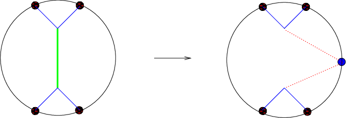
These recursion relations are shown schematically in Fig. 2. Say we set out to compute a four-point vacuum-vacuum correlator. A typical Witten diagram involves three ingredients: a bulk-bulk propagator shown by the heavy line in the middle (green), four insertions of a source on the boundary shown by the small crosshatched circles, and four bulk-boundary propagators shown by the lines from the boundary to the bulk (blue). The recursion relations (65) convert this to the integrated product of two three-point functions. This is done by cutting open the bulk-bulk propagator and replacing it with a product of two normalizable modes shown by the dotted lines (red). Since these modes are normalizable the small solid circle (blue) on the boundary is not really the insertion of a source but represents a coherent state. We need to integrate over the momentum running through these normalizable modes, which reproduces the result of the sum of Witten diagrams.

Note that the crucial ingredient in our derivation above was the leading large $w$ behaviour of the integrand. In particular, we need the ${\text{O}}\left({w}\right)$ piece, but to derive the results above, we do not need the ${\text{O}}\left({1}\right)$ or ${\text{O}}\left({1\over w}\right)$ pieces. There is another route to this method that is somewhat more direct. Instead of using the background field method, we can just do perturbation theory in q-lightcone gauge for the gauge-field. In this gauge, the ${\boldsymbol{q}}w$ momentum does not propagate in the numerator; so it is clear that every propagator comes with a factor of ${1\over w}$ . Except for the unique vertex mentioned above, there are also no interaction vertices that are proportional to $w$ in this gauge. This immediately leads to the ${\text{O}}\left({w}\right)$ term above. As long as one of the polarization vectors is ${\boldsymbol{q}}$ , this analysis together with the Ward identity (48) is enough to derive the falloff of the integrand at large $w$ .

4.3 Gravity

We now turn to the case of graviton scattering. Say that we are considering a n-point transition amplitude $T({\boldsymbol{k_{1}}},\ldots{\boldsymbol{k_{n}}})$ . To analyze the amplitude when we BCFW extend ${\boldsymbol{k_{1}}}\rightarrow{\boldsymbol{k_{1}}}+{\boldsymbol{q}}w$ and ${\boldsymbol{k_{n}}}\rightarrow{\boldsymbol{k_{n}}}-{\boldsymbol{q}}w$ , we go to background field gauge where we consider the two-point function of gravitons with these momenta in a background of soft gravitons with momenta ${\boldsymbol{k_{2}}},\ldots{\boldsymbol{k_{n-1}}}$ .

We have already expanded the gravity action about a classical background in (32). However, we need to be cautious because the background metric now also contains the fluctuations induced by the gravitons with momenta ${\boldsymbol{k_{2}}},\ldots{\boldsymbol{k_{n}}}$ . To differentiate it from the AdS metric, below, we will denote it by $g^{b}_{\mu\nu}$ ( $b$ stands for background) and its inverse by $g_{b}^{\mu\nu}$ . After adding the background gauge-fixing term, the gravity action becomes

S={-1\over 64\pi G}\int_{{\boldsymbol{x}},z}\sqrt{-g_{b}}\left(g_{b}^{\mu\rho}g_{b}^{\nu\sigma}g_{b}^{\alpha\beta}\nabla_{\alpha}\tilde{h}_{\rho\sigma}\nabla_{\beta}h_{\mu\nu}+2\tilde{h}_{\mu_{1}\nu_{1}}R_{\mu\rho\nu\sigma}h_{\alpha\beta}g_{b}^{\mu\mu_{1}}g_{b}^{\nu\nu_{1}}g_{b}^{\rho\alpha}g_{b}^{\beta\sigma}\right),

(66)

up to boundary terms, which do not affect the bulk Green’s functions and where we have written the factors of the inverse metric explicitly for reasons that will shortly become clear.

It is convenient to break up the background metric into a “pure” AdS part and another part that comes from the fluctuations caused by the gravitons in our amplitude. We write

H^{\mu\nu}\equiv{g_{b}^{\mu\nu}-g^{\mu\nu}},

(67)

where $g^{\mu\nu}$ is the inverse of the metric in (1). We choose q-lightcone gauge, which means that

q_{\mu}H^{\mu\nu}=0.

(68)

The split in (67) is not arbitrary since the AdS metric is the zero-momentum part of the background.

Now, we work with the propagator (44), which corresponds to treating the AdS part of the quadratic action exactly but the $H^{\mu\nu}$ as a perturbation. Note that if we were to expand out (66), in terms of ${\boldsymbol{H}}$ the answer would be inordinately complicated. Fortunately, we are only interested in the ${\text{O}}\left({w^{2}}\right)$ part of the amplitude and this is easy to determine.

As above, there is a unique set of diagrams that contribute to this action. In these, $H^{\mu\nu}$ carries the momentum $-{\boldsymbol{k_{1}}}-{\boldsymbol{k_{n}}}=\sum_{i=2}^{n-1}{\boldsymbol{k_{i}}}$ for which (68) cannot be chosen. The leading ${\text{O}}\left({w^{2}}\right)$ part of the transition amplitude then comes from

\int_{{\boldsymbol{x}},z}\sqrt{-g_{b}}\left[H^{\mu\nu}(-{\boldsymbol{k_{1}}}-{\boldsymbol{k_{n}}},z)q_{\mu}q_{\nu}w^{2}g^{\rho\sigma}g^{\alpha\beta}h_{\rho\alpha}({\boldsymbol{k_{1}}}+qw,z)h_{\sigma\beta}({\boldsymbol{k_{n}}}-qw,z)+{\text{O}}\left({w}\right)\right].

(69)

Note that we have performed the ${\boldsymbol{x}}$ integral and imposed momentum conservation. So, the functions ${\boldsymbol{H}}$ and ${\boldsymbol{h}}$ in the expression above are written as functions of the momenta and the radial coordinate only.

As in the case of gauge fields above, this result may be alternately derived by going to q-lightcone gauge from the start. Note that the terms that appear at ${\text{O}}\left({w}\right)$ and ${\text{O}}\left({1}\right)$ above are significantly more complicated than in flat-space, but we do not need their explicit forms.

Consider the case where the polarization for $h_{\mu\nu}({\boldsymbol{k_{1}}}+qw,z)$ , as defined in (43) is $\epsilon^{1}_{\mu\nu}=q_{\mu}q_{\nu}$ . With $\psi_{1}$ defined by

\psi_{1}({\boldsymbol{x}},z)\equiv z^{-2}E_{d\over 2}({\boldsymbol{k_{1}}},z)e^{i({\boldsymbol{k_{1}}}+qw)\cdot{\boldsymbol{x}}},

(70)

we can write (after restoring the ${\boldsymbol{x}}$ dependence in ${\boldsymbol{h}}$ )

\begin{split}h_{\mu\nu}({\boldsymbol{k_{1}}}+{\boldsymbol{q}}w,{\boldsymbol{x}},z)&=q_{\mu}q_{\nu}z^{-2}E_{d\over 2}({\boldsymbol{k}}_{1},z)e^{i({\boldsymbol{k_{1}}}+{\boldsymbol{q}}w)\cdot{\boldsymbol{x}}}\\ &={1\over w}\left(\nabla_{(\mu}{q_{\nu)}\psi_{1}}-k_{1(\mu}q_{\nu)}\psi_{1}-\delta_{(\mu}^{0}q_{\nu)}{\partial\psi_{1}\over\partial z}-\Gamma_{\mu\nu}^{\rho}q_{\rho}\psi_{1}\right)\\ &={1\over w}\left(\nabla_{(\mu}{q_{\nu)}\psi_{1}}-k_{1(\mu}q_{\nu)}\psi_{1}-\delta_{(\mu}^{0}q_{\nu)}{\partial\psi_{1}\over\partial z}+2q_{(\mu}\delta_{\nu)}^{0}{\psi_{1}\over z}\right)\\ &\equiv{1\over w}\nabla_{(\mu}{q_{\nu)}\psi_{1}}-{1\over w}q_{(\mu}t_{\nu)},\end{split}

(71)

where the last line defines a vector field ${\boldsymbol{t}}({\boldsymbol{x}},z)$ , and we have used (33) to go from the first to the second line. However, since the dependence of ${\boldsymbol{t}}$ on ${\boldsymbol{x}}$ continues to be of the form $e^{i({\boldsymbol{k_{1}}}+{\boldsymbol{q}}w)\cdot{\boldsymbol{x}}}$ , this itself may be further rewritten using

{1\over w}q_{(\mu}t_{\nu)}={1\over w^{2}}\left(\nabla_{(\mu}t_{\nu)}-k_{1(\mu}t_{\nu)}-{\delta_{(\mu}^{0}\partial t_{\nu)}\over\partial z}-\Gamma^{\rho}_{\mu\nu}t_{\rho}\right)\equiv{1\over w^{2}}\nabla_{(\mu}t_{\nu)}+{1\over w^{2}}t^{(2)}_{\mu\nu}(x,z),

(72)

where $t^{(2)}_{\mu\nu}$ is a symmetric tensor field that is defined by the equation above. The Ward identity (49) now tells us that instead of using $h_{\mu\nu}({\boldsymbol{k_{1}}}+{\boldsymbol{q}}w,x,z)$ , we can instead use ${1\over w^{2}}t^{(2)}_{\mu\nu}(x,z)$ in (69).

Next, note that $h_{\mu\nu}({\boldsymbol{k_{n}}}-{\boldsymbol{q}}w,x,z)$ does not itself grow at large $w$ , provided it has a polarization that is orthogonal to ${\boldsymbol{q}}$ . So, we see that the following conditions are sufficient for the integrand to behave well:

1.

$\epsilon^{n}_{\mu\nu}t^{(2)}_{\rho\sigma}g^{\mu\rho}g^{\nu\sigma}=0$ ,
2.

$\epsilon^{n}_{\mu\nu}q_{\rho}g^{\mu\rho}=0$ .

There is an additional possibility. If ${\boldsymbol{\epsilon^{n}}}$ itself has a factor of ${\boldsymbol{q}}$ then we can repeat (71) to pull down another factor of ${1\over w}$ . In that case, condition 2 above is automatically satisfied but we can relax condition 1.

Hence, we see that the graviton transition amplitude is well behaved under the following conditions:

1.

$\epsilon^{n}_{ij}=q_{(i}v_{j)},$ where ${\boldsymbol{v}}\cdot{\boldsymbol{q}}=0$ or
2.

$\epsilon^{n}_{ij}=v^{1}_{(i}v^{2}_{j)},$ where ${\boldsymbol{v^{m}}}\cdot{\boldsymbol{q}}={\boldsymbol{v^{m}}}\cdot{\boldsymbol{k_{1}}}=0$ .

The first set above includes the case where ${\boldsymbol{v}}={\boldsymbol{q}}$ . Also, just the requirement that ${\boldsymbol{\epsilon^{n}}}$ be a valid polarization vector implies that ${\boldsymbol{v}}\cdot{\boldsymbol{k_{n}}}={\boldsymbol{v^{1}}}\cdot{\boldsymbol{v^{2}}}={\boldsymbol{v^{1}}}\cdot{\boldsymbol{k_{n}}}={\boldsymbol{v^{2}}}\cdot{\boldsymbol{k_{n}}}=0$ . Of course, we can interchange the role of ${\boldsymbol{\epsilon^{1}}}$ and ${\boldsymbol{\epsilon^{n}}}$ above. So, if we take $\epsilon^{n}_{ij}=q_{i}q_{j}$ , then we can have $\epsilon^{1}_{ij}=q_{(i}v_{j)},$ where ${\boldsymbol{v}}\cdot{\boldsymbol{q}}={\boldsymbol{v}}\cdot{\boldsymbol{k_{1}}}=0$ or $\epsilon^{1}_{ij}=v^{1}_{(i}v^{2}_{j)},$ where ${\boldsymbol{v^{m}}}\cdot{\boldsymbol{q}}={\boldsymbol{v^{m}}}\cdot{\boldsymbol{k_{n}}}={\boldsymbol{v^{m}}}\cdot{\boldsymbol{k_{1}}}=0$ .

With these conditions on the polarization vectors we find the following recursion relations

\begin{split}&T({\boldsymbol{k_{1}}},{\boldsymbol{\epsilon_{1}}},\ldots{\boldsymbol{k_{n}}},{\boldsymbol{\epsilon_{n}}})=\sum_{\{\pi\},m,{\boldsymbol{\epsilon_{m}^{\prime}}}}\int{-i{\cal T}^{2}\over 2(p^{2}+{\boldsymbol{K}}^{2})}dp^{2},\\ &{\cal T}^{2}\equiv{T({\boldsymbol{k_{1}}}(p),{\boldsymbol{\epsilon_{1}}},\ldots{\boldsymbol{k_{m}^{\prime}}},{\boldsymbol{\epsilon_{m}^{\prime}}})T(-{\boldsymbol{k_{m}^{\prime}}},{\boldsymbol{\epsilon_{m}^{\prime}}},\ldots{\boldsymbol{k_{n}}}(p),{\boldsymbol{\epsilon_{n}}})}.\end{split}

(73)

The sum over ${\boldsymbol{k_{m}^{\prime}}}$ is again over all valid polarization vectors for this momentum and the other quantities in (73) are defined the same way as in (65) and (56). In particular, the definitions of (57) continue to apply. These recursion relations are structurally identical to (65) although we should remember that each polarization vector, ${\boldsymbol{\epsilon_{m}}}$ , above is a two-index tensor in (73), and only a vector in (65).

4.4 Polarization Vectors

As we have pointed out above, given a transition amplitude with some external polarization vectors, we cannot typically compute it by means of a single BCFW extension. However, since the amplitude depends linearly on the polarization vectors, we can often decompose it into a sum over amplitudes, each of which behaves well under some BCFW extension.

To see this more clearly, say that we are interested in a correlator of operators $O^{I}$ where the capital $I$ index indicates that these operators transform in some representation of $SO(d-1,1)$ . A n-point correlator of these operators can be written as

T^{I_{1}\ldots I_{n}}({\boldsymbol{k_{1}}},\ldots{\boldsymbol{k_{n}}})\equiv\langle O^{I_{1}}({\boldsymbol{k_{1}}})\ldots O^{I_{n}}({\boldsymbol{k_{n}}})\rangle,

(74)

where $T^{I_{1}\ldots I_{n}}$ is some tensor of the Lorentz group. Computing the correlator is the same as computing all components of ${\boldsymbol{T}}$ .

There are further constraints on the (74). For example, it must be invariant under a simultaneous interchange of ${\boldsymbol{k_{m}}}$ and ${\boldsymbol{k_{n}}}$ , and $I_{m}$ and $I_{n}$ . Second, ${\boldsymbol{T}}$ must be conserved with respect to each momentum when we are dealing with conserved currents or the stress tensor. There are many additional constraints [38] that come from conformal invariance, which strongly restrict the form of ${\boldsymbol{T}}$ in (74) for small $n$ . However, these are easier to see in position space, and we will not use them in this section.

If we dot (74) with some external polarization vectors, ${\boldsymbol{\epsilon^{1}}},\ldots{\boldsymbol{\epsilon^{n}}}$ , we find

\langle O^{I_{1}}({\boldsymbol{k_{1}}})\ldots O^{I_{n}}({\boldsymbol{k_{n}}})\epsilon^{1}_{I_{1}}\ldots\epsilon^{n}_{I_{n}}\rangle=T^{I_{1}\ldots I_{n}}({\boldsymbol{k_{1}}},\ldots{\boldsymbol{k_{n}}})\epsilon^{1}_{I_{1}}\ldots\epsilon^{n}_{I_{n}}.

(75)

If we had some means of computing the left hand side for arbitrary polarizations, this would enable us to extract all the components of ${\boldsymbol{T}}$ . However, the BCFW extension that we have described above puts constraints on the polarization vectors. Can we recover information about all components by combining different pairs of BCFW extensions?

We will consider the four-point function in detail below. As we mentioned above, there are dynamical constraints on this correlator; however, we will only focus on the fact that it must be conserved. This is because if we can show, without using any other dynamical information, that all possible components of ${\boldsymbol{T}}$ in (74) in a four-point function are accessible by our methods, then this would be sufficient to show that arbitrary n-point correlators are also accessible.

To see this, consider what happens if we add a fifth index to (74). The recursion relations (65) and (73) place constraints only on pairs of polarization vectors. So, if all possible four-point tensor structures are calculable by choosing and extending pairs from ${\boldsymbol{k_{1}}}\ldots{\boldsymbol{k_{4}}}$ , then we can choose the polarization vector for ${\boldsymbol{k_{5}}}$ arbitrarily. Moreover, every allowed conserved five-index tensor can be written as

T^{I_{1}\ldots I_{5}}({\boldsymbol{k_{1}}},\ldots{\boldsymbol{k_{5}}})=\sum_{\alpha}T_{\alpha}^{I_{1}\ldots I_{4}}({\boldsymbol{k_{1}}},\ldots{\boldsymbol{k_{5}}})v_{\alpha}^{I_{5}}({\boldsymbol{k_{1}}},\ldots{\boldsymbol{k_{5}}}),

(76)

where $v_{\alpha}$ is a list of vector functions, which are orthogonal to ${\boldsymbol{k_{5}}}$ , indexed by $\alpha$ . Evidently, if we can choose the polarization vector ${\boldsymbol{\epsilon^{5}}}$ arbitrarily and we can also access all tensors $T_{\alpha}^{I_{1}\ldots I_{4}}$ , then we can also access any five-index tensor.

While the computability of all four-point tensor structures is sufficient to ensure the computability of higher-point structures, it is not necessary. In some cases (such as gravity in $d=5$ ), as we will see below, it is not possible to compute all possible tensor-structures for the four-point correlator. However, adding additional particles now gives us more choices of BCFW extensions and, for a sufficient number of external particles, we can once again access all allowed tensor structures.

4.4.1 Polarizations for Gauge Bosons

Let us start with the case of $d=4$ . For each momentum, ${\boldsymbol{k_{m}}}$ , there are three allowed polarization vectors. So, a four-point correlator ${\boldsymbol{T}}$ has, a priori, $3^{4}=81$ possible components. On the other hand, given a pair of momenta, say ${\boldsymbol{k_{1}}}$ and ${\boldsymbol{k_{4}}}$ , there are two choices of ${\boldsymbol{q}}$ , which we denote by ${\boldsymbol{q^{1}}}$ and ${\boldsymbol{q^{2}}}$ . The constraints worked out in subsection 4.2 now tell us that we either take ${\boldsymbol{\epsilon^{1}}}={\boldsymbol{q^{1}}},{\boldsymbol{\epsilon^{4}}}={\boldsymbol{q^{1}}}$ or ${\boldsymbol{\epsilon^{1}}}={\boldsymbol{q^{2}}},{\boldsymbol{\epsilon^{4}}}={\boldsymbol{q^{2}}}$ . The polarization vectors for ${\boldsymbol{k_{2}}}$ and ${\boldsymbol{k_{3}}}$ can be arbitrary and there are $3\times 3=9$ combinations of these. So, extending momenta ${\boldsymbol{k_{1}}}$ and ${\boldsymbol{k_{4}}}$ should allow us to compute $2\times 9=18$ components of ${\boldsymbol{T}}$ .

We can choose 6 distinct pairs with 4 particles. So, by making all possible BCFW extensions we get $18\times 6=108$ pieces of data about the components of ${\boldsymbol{T}}$ . One would naively think that this forms an overcomplete basis for the $81$ numbers that we wish to extract. However, this is a little too quick. This is because, if ${\boldsymbol{T}}$ is of the form

T^{i_{1}i_{2}i_{3}i_{4}}=\epsilon^{j_{1}j_{2}j_{3}j_{4}}\left(\delta_{j_{1}}^{i_{1}}-{k_{1j_{1}}k_{1}^{i_{1}}\over{\boldsymbol{k_{1}}}^{2}}\right)\left(\delta_{j_{2}}^{i_{2}}-{k_{2j_{2}}k_{2}^{i_{2}}\over{\boldsymbol{k_{2}}}^{2}}\right)\left(\delta_{j_{3}}^{i_{3}}-{k_{3j_{3}}k_{3}^{i_{3}}\over{\boldsymbol{k_{3}}}^{2}}\right)\left(\delta_{j_{4}}^{i_{4}}-{k_{4j_{4}}k_{4}^{i_{4}}\over{\boldsymbol{k_{4}}}^{2}}\right),

(77)

it will be invisible to all our choices of BCFW extension. So, we can compute only 80 components of ${\boldsymbol{T}}$ using all 6 BCFW extensions. Fortunately, this is not a problem since the choice of ${\boldsymbol{T}}$ in (77) is completely antisymmetric under the simultaneous exchange of any pair of indices and momenta. For example, interchanging $({\boldsymbol{k_{1}}},i_{1})$ and $({\boldsymbol{k_{2}}},i_{2})$ changes the sign of (77). Consequently, this tensor structure is inconsistent with the symmetries of the correlator and is not allowed. So, we can compute all possible tensor structures in correlators of conserved currents, in $d=4$ , by means of the BCFW extension.

We now turn to $d=5$ . Each momentum has $4$ possible associated polarization vectors; so ${\boldsymbol{T}}$ has, a priori, a total of $4^{4}=256$ components for a four-point correlator. Given a pair of momenta, say ${\boldsymbol{k_{1}}}$ and ${\boldsymbol{k_{4}}}$ , we now have a continuous family of choices for ${\boldsymbol{q}}$ . Moreover, if we choose ${\boldsymbol{\epsilon^{1}}}={\boldsymbol{q}}$ , we can also take ${\boldsymbol{\epsilon^{4}}}={\boldsymbol{v^{4}}}$ , where ${\boldsymbol{v^{4}}}$ is a vector orthogonal to ${\boldsymbol{q}}$ and ${\boldsymbol{k_{4}}}$ . Similarly, by taking ${\boldsymbol{\epsilon^{4}}}={\boldsymbol{q}}$ , we can take ${\boldsymbol{\epsilon^{1}}}={\boldsymbol{v^{1}}}$ , orthogonal to ${\boldsymbol{q}}$ and ${\boldsymbol{k_{1}}}$ . The polarizations for ${\boldsymbol{k_{2}}}$ and ${\boldsymbol{k_{3}}}$ can, again, be arbitrary. Focusing, momentarily, only on the indices corresponding to $i_{1}$ and $i_{4}$ , a general 2-index conserved tensor can be written as

T^{i_{1}i_{4}}=T_{\text{tl}}^{i_{1}i_{4}}+A\eta^{j_{1}j_{4}}\left(\delta^{i_{1}}_{j_{1}}-{k_{1}^{i_{1}}k_{1j_{1}}\over{\boldsymbol{k_{1}}}^{2}}\right)\left(\delta^{i_{4}}_{j_{4}}-{k_{4}^{i_{4}}k_{4j_{4}}\over{\boldsymbol{k_{4}}}^{2}}\right),

(78)

where $A$ is some constant and ${\boldsymbol{T_{\text{tl}}}}$ is (a) traceless and (b) conserved with respect to both ${\boldsymbol{k_{1}}}$ and ${\boldsymbol{k_{4}}}$ . The polarization-combinations above allow us to detect all components of ${\boldsymbol{T}}_{\text{tl}}$ but are insensitive to the presence of $A$ .

Since ${\boldsymbol{T_{\text{tl}}}}$ has 8 components, making all possible choices of polarizations for ${\boldsymbol{k_{2}}}$ and ${\boldsymbol{k_{3}}}$ gives us $8\times 16=108$ pieces of data. Now, making all 6 possible BCFW extensions gives us $6\times 108=648$ pieces of data. Also, for gauge bosons in $d=5$ , there is no inaccessible tensor like (77). So, by making all possible BCFW extensions, we obtain an overcomplete set of equations for the $256$ allowed components of ${\boldsymbol{T}}$ that can all, hence, be determined.

The calculation for $d\geq 6$ goes as follows. There are $d-1$ possible polarizations for each momentum leading to $(d-1)^{4}$ independent components. Given a pair ${\boldsymbol{k_{1}}},{\boldsymbol{k_{4}}}$ we now not only have a $d-4$ parameter continuous family of choices for ${\boldsymbol{q}}$ , we can also choose ${\boldsymbol{v^{1}}}$ and ${\boldsymbol{v^{4}}}$ in several different ways provided we keep them orthogonal to ${\boldsymbol{q}}$ . Hence, just as above, in the $i_{1},i_{4}$ space we can detect all tensors that are conserved with respect to ${\boldsymbol{k_{1}}}$ and ${\boldsymbol{k_{4}}}$ and are traceless. There are $(d-2)^{2}-1$ linearly independent tensors of this sort. So, one BCFW extension gives us $(d-1)^{2}\left[(d-2)^{2}-1\right]$ pieces of data. The six possible BCFW extensions give us $6(d-1)^{2}\left[(d-2)^{2}-1\right]$ pieces of data that form an overcomplete set for the $(d-1)^{4}$ independent allowed components of ${\boldsymbol{T}}$ in $d$ -dimensions.⁵⁵ 5 In fact, we have already seen that ${d\choose 4}$ of these components must be zero. However, we have to put this in from the start only for $d=4$ ; in higher $d$ , the recursion relations will allow us to compute these components and verify that they vanish.

4.4.2 Polarizations for Gravitons

We now turn to the case of gravity. We start with $d=4$ and then go on to higher $d$ . As we will see below this analysis has similarities but also important differences with the analysis for gauge bosons.

Polarization vectors for a graviton with momentum ${\boldsymbol{k}}$ are given by symmetric traceless tensors that are orthogonal to ${\boldsymbol{k}}$ . In $d=4$ , this implies that we have 5 possible polarizations for each momentum. As we pointed out above, if we extend ${\boldsymbol{k_{1}}}$ and ${\boldsymbol{k_{4}}}$ there are two possible choices of ${\boldsymbol{q}}$ , which we denote by ${\boldsymbol{q^{1}}}$ and ${\boldsymbol{q^{2}}}$ . If we choose the polarization vector for particle ${\boldsymbol{k_{1}}}$ by $\epsilon^{1}_{ij}=q_{i}q_{j}$ , (where ${\boldsymbol{q}}$ is either of the two allowed choices) then we must choose $\epsilon^{4}_{ij}=q_{i}q_{j}$ or $\epsilon^{4}_{ij}=q_{(i}v^{4}_{j)}$ , where, as above, ${\boldsymbol{v^{4}}}$ is a vector orthogonal to ${\boldsymbol{q}}$ and ${\boldsymbol{k_{4}}}$ . The choice of $\epsilon^{4}_{ij}=q_{i}q_{j}$ also behaves well under the BCFW extension if we choose $\epsilon^{1}_{ij}=q_{(i}v^{1}_{j)}$ , where ${\boldsymbol{v^{1}}}$ is orthogonal to ${\boldsymbol{q}}$ and ${\boldsymbol{k_{1}}}$ . The polarizations for ${\boldsymbol{k_{2}}}$ and ${\boldsymbol{k_{3}}}$ can be arbitrary.

So, extending ${\boldsymbol{k_{1}}}$ and ${\boldsymbol{k_{4}}}$ by ${\boldsymbol{q^{1}}}$ allows us to calculate $3\times 25=75$ combinations of polarizations. Extending ${\boldsymbol{k_{1}}}$ and ${\boldsymbol{k_{4}}}$ by ${\boldsymbol{q^{2}}}$ allows us to calculate another 75. So, with all 6 possible BCFW extensions we can compute $6\times(75+75)=900$ polarization-combinations. Naively, this would seem to give an overcomplete set for the 625 distinct components of ${\boldsymbol{T}}$ .

However, as above, this is not quite correct. In particular, consider a ${\boldsymbol{T}}$ of the form

T^{i_{1}j_{1}\ldots i_{4}j_{4}}=S_{1234}\left[\epsilon^{i_{1}\ldots i_{4}}\epsilon^{j_{1}\ldots j_{4}}\right],

(79)

where the operator $S_{1234}$ symmetrizes its argument in $(i_{1},j_{1}),(i_{2},j_{2}),(i_{3},j_{3}),(i_{4},j_{4})$ , makes it traceless in these pairs, and projects the $(i_{m},j_{m})$ component orthogonal to ${\boldsymbol{k_{m}}}$ . The ${\boldsymbol{T}}$ in (79) cannot be detected by any of the 900 BCFW extensions described above. Moreover, unlike in the case of gauge bosons, this tensor is symmetric under the simultaneous interchange of Lorentz indices and momenta. For example, if we interchange $(i_{1},j_{1})$ and $(i_{4},j_{4})$ , and also interchange ${\boldsymbol{k_{1}}}$ and ${\boldsymbol{k_{4}}}$ then ${\boldsymbol{T}}$ returns to itself, because each $\epsilon$ tensor contributes a factor of $(-1)$ leading to an overall factor of unity. We are also not aware of any other argument that would allow us to exclude this term. So, more precisely, the BCFW procedure allows us to compute 624 out of the 625 components of a general ${\boldsymbol{T}}$ .

It would be interesting to understand the coefficient of this term for the four-point function of stress-tensors given Einstein gravity in AdS₅. Also, it would be nice if conformal invariance or other restrictions allowed us to fix this term; the studies of [27, 26] might be useful in this context.

Notice that this problem does not occur for five- and higher-point amplitudes in $d=4$ . There is no tensor, in four dimensions, that is completely antisymmetric in five indices. So, for higher-point amplitudes it seems possible to compute any polarization-combination using the BCFW extension.

We now turn to $d=5$ . Each momentum has $9$ possible associated polarization vectors; hence, ${\boldsymbol{T}}$ has a total of $9^{4}=729$ components for a four-point correlator. The important difference from $d=4$ is that given a pair of momenta, say ${\boldsymbol{k_{1}}}$ and ${\boldsymbol{k_{4}}}$ , we now have a continuous family of choices for ${\boldsymbol{q}}$ . Once again, if we choose $\epsilon^{1}_{ij}=q_{i}q_{j}$ , we can take ${\boldsymbol{\epsilon^{4}}}={\boldsymbol{\epsilon^{1}}}$ or $\epsilon^{4}_{ij}=q_{(i}v^{4}_{j)}$ . In $d=6$ and higher, as we will see below, we have additional choices for ${\boldsymbol{\epsilon^{4}}}$ that are not available here. This is because in $d=6$ (or higher), there are two (or more) linearly independent vectors that are orthogonal to ${\boldsymbol{q}}$ , ${\boldsymbol{k_{1}}}$ and ${\boldsymbol{k_{4}}}$ .

Let us focus, momentarily, only on the indices corresponding to ${\boldsymbol{k_{1}}}$ , which are $i_{1},j_{1}$ , and the indices corresponding ${\boldsymbol{k_{4}}}$ , which are $i_{4},j_{4}$ . For the sake of simplicity in this analysis, we also assume (without loss of generality for our purposes) that ${\boldsymbol{k_{1}}}$ is orthogonal to ${\boldsymbol{k_{4}}}$ .

First, we consider the number of linearly independent polarization-combinations we can obtain by taking ${\boldsymbol{\epsilon}}^{1}_{ij}=q_{i}q_{j}$ and ${\boldsymbol{\epsilon}}^{4}_{ij}=q_{i}q_{j}$ or ${\boldsymbol{\epsilon}}^{4}_{ij}=q_{i}v^{4}_{j}$ and let us, for the sake of illustration, also choose ${\boldsymbol{v_{4}}}$ to be orthogonal to all three ${\boldsymbol{k_{1}}},{\boldsymbol{k_{4}}}$ and ${\boldsymbol{q}}$ . If the indices $i_{1},j_{1},i_{4},j_{4}$ run only over the three-dimensional subspace orthogonal to ${\boldsymbol{k_{1}}}$ and ${\boldsymbol{k_{4}}}$ , then given a tensor that is symmetric and traceless in each of $(i_{1},j_{1})$ and $(i_{4},j_{4})$ we can write

T^{i_{1}j_{1}i_{4}j_{4}}=T_{(4)}^{i_{1}i_{4}j_{1}j_{4}}+\epsilon^{i_{1}i_{4}l}T_{(3)}^{lj_{1}j_{4}}+\delta^{i_{1}i_{4}}T_{(2)}^{j_{1}j_{4}}+\delta^{i_{1}i_{4}}T_{(1)}^{j_{1}j_{4}}+T_{(0)}\delta^{i_{1}i_{4}}\delta^{j_{1}j_{4}}+(i_{1}\leftrightarrow j_{1})+(i_{4}\leftrightarrow j_{4}).

(80)

Here the subscript under each tensor indicates which representation of $SO(3)$ it belongs to. (The $SO(3)$ is the group of rotations in the three-dimensional space orthogonal to ${\boldsymbol{k_{1}}}$ and ${\boldsymbol{k_{4}}}$ .) So ${\boldsymbol{T_{(4)}}},{\boldsymbol{T_{(3)}}},{\boldsymbol{T_{(2)}}}$ are completely symmetric and traceless in any pair of indices and ${\boldsymbol{T_{(1)}}}$ is antisymmetric.

By just using $\epsilon^{1}_{ij}=q_{i}q_{j}$ and $\epsilon^{4}_{ij}=q_{i}q_{j}$ , we can completely extract the ${\boldsymbol{T_{(4)}}}$ term in (80). To see this, note that, in this orthogonal 3 dimensional subspace, we can choose $q$ as

q=(1,{x^{2}-1\over 2ix},{x^{2}+1\over 2x}).

(81)

Dotting ${\boldsymbol{T}}$ with four-copies of $q$ we find

T^{i_{1}j_{1}i_{4}j_{4}}q_{i_{1}}q_{j_{1}}q_{i_{4}}q_{j_{4}}=T_{(4)}^{i_{1}j_{1}i_{4}j_{4}}q_{i_{1}}q_{j_{1}}q_{i_{4}}q_{j_{4}}.

(82)

We can extract the coefficients of $x^{4},x^{3},\ldots x^{-3},x^{-4}$ in this dot product by allowing $x$ to run over various values. More precisely, we could take $x=e^{i\theta}$ and Fourier transform in $\theta$ that would give us these 9 different coefficients. These correspond exactly to the 9 different components of ${\boldsymbol{T_{(4)}}}$ . Now, consider taking ${\boldsymbol{v^{4}}}$ to be orthogonal to both ${\boldsymbol{k_{1}}}$ and ${\boldsymbol{k_{4}}}$ . If we now take $\epsilon^{4}_{ij}=q_{(i}v^{4}_{j)}$ , with ${\boldsymbol{v^{4}}}$ orthogonal to both ${\boldsymbol{k_{1}}}$ and ${\boldsymbol{k_{4}}}$ then we can also extract the ${\boldsymbol{T_{(3)}}}$ term in (80). This gives us 7 more terms.

So far we have considered tensors that are orthogonal to both ${\boldsymbol{k_{1}}}$ and ${\boldsymbol{k_{4}}}$ . However, we are also allowed tensors of the form

(T^{\prime})_{(3)}^{i_{1}j_{1}i_{4}1}+(T^{\prime})_{(3)}^{i_{1}j_{1}1i_{4}}

This tensor has one leg along the direction of ${\boldsymbol{k_{1}}}$ , which is indicated by the index $1$ in the superscript, and the other indices $i_{1},j_{1},i_{4}$ run in the space orthogonal to both ${\boldsymbol{k_{1}}}$ and ${\boldsymbol{k_{4}}}$ . We have chosen this tensor to be completely symmetric in these three-indices and placed a prime-symbol on it to distinguish it from the ${\boldsymbol{T_{(3)}}}$ that appeared above. This is an allowed tensor structure because it is conserved (recall that we have taken ${\boldsymbol{k_{1}}}\cdot{\boldsymbol{k_{4}}}=0$ ) and, by construction, it is symmetric in its last two indices. By taking ${\boldsymbol{v^{4}}}={\boldsymbol{k_{1}}}$ We can now extract the 7 components of this tensor.

If we also take $\epsilon^{4}_{ij}=q_{i}q_{j}$ and allow $\epsilon^{1}_{ij}=q_{i}v^{1}_{j}$ , then we get a total of $9+7\times 4=37$ components. Combining the $81$ polarizations from $\epsilon^{2},\epsilon^{3}$ we get $37\times 81=2997$ components. The six different BCFW extensions lead us to $2997\times 6=17982$ different polarization-combinations, which would seem to form a highly overcomplete basis for the $9^{4}=6561$ distinct possibilities.

However, we need to be careful. As above, any tensor of the form (all indices now again run over all 5 dimensions)

T^{i_{1}j_{1}\ldots i_{4}j_{4}}=S_{1234}\left[A_{1}^{i_{1}\ldots i_{4}}A_{2}^{j_{1}\ldots j_{4}}\right],

(83)

where $A_{1},A_{2}$ are tensors that are antisymmetric in any interchange of indices, cannot be detected by BCFW extensions.

Even with a five-point correlator, we cannot detect the part of the correlation function that is proportional to

T^{i_{1}j_{1}\ldots i_{5}j_{5}}=S_{12345}\left[\epsilon^{i_{1}\ldots i_{5}}\epsilon^{j_{1}\ldots j_{5}}\right].

(84)

So, in this case, we can get only $9^{5}-1$ out of the $9^{5}$ distinct polarization combinations. For six- and higher-point correlators, there are no completely antisymmetric tensors and we can get all possible polarizations using the BCFW extension.

We will not explicitly work out the combinatorics for $d=6$ and higher since they are very similar to the calculations above. One important distinction is if we choose $\epsilon^{1}_{ij}=q_{i}q_{j}$ , we can choose $\epsilon^{4}_{ij}=v^{41}_{(i}v^{42}_{j)}$ where ${\boldsymbol{v^{41}}}\cdot{\boldsymbol{v^{42}}}=0$ and both these vectors are orthogonal to $q,{\boldsymbol{k_{1}}},{\boldsymbol{k_{4}}}$ . This allows us to also detect tensors of the form (83) or (84). So, for $d=6$ or higher, we can compute all polarization-combinations using the BCFW extension.

5 Supersymmetric Theories

We now turn to the generalization of these recursion relations to theories with supersymmetry. In this section we will use the easily derived fact that as long as the particles that we are BCFW extending are gravitons or gauge bosons, the behaviour of the amplitude at $w\rightarrow\infty$ is not affected by the presence of additional matter particles. Moreover, (65) and (73) continue to hold for Yang-Mills theory and gravity coupled to matter with the modification that the sum over polarizations must be expanded to run over these particles as well.

The basic idea here is the same as the one used in the extension of the BCFW-recursion relations to supersymmetric theories in flat-space [39, 7, 40]. As we have pointed out above, the behaviour under BCFW extension of amplitudes with external gravitons or gauge bosons is better than that of amplitudes with external scalars or fermions. In fact, if we BCFW-extend external scalars, our recursion relations would involve an unwieldy boundary term that would need to be calculated explicitly using Witten diagrams.⁶⁶ 6 We should mention here that the physical intuition that underlies this paper: the fact that BCFW-deformed amplitudes are dominated by interactions at a small number of points, was also used to study these amplitudes in Yang-Mills theory coupled to matter. If we consider a single BCFW-extended matter-line interacting with gauge bosons, the powers of $w$ in the amplitude are correlated with the number of color-generators that appear. This leads to some surprising cancellations in gauge theories with matter at one-loop [40, 41].

In theories with supersymmetry, however, we can relate amplitudes involving external matter particles to amplitudes involving gluons or gravitons. In flat-space, in ${{\mathcal{N}}=4}$ SYM ( ${{\mathcal{N}}=8}$ SUGRA), we can always convert at least two particles in a scattering amplitude to negative helicity gluons (gravitons) [39, 7]. In theories with less supersymmetry, such as ${{\mathcal{N}}=2}$ SYM, we can still convert two particles, either to negative helicity gluons or to positive helicity gluons [40].

In AdS, the situation is somewhat different. In $d=4$ , for example, the constraints on the polarization vectors for gauge bosons that we have enumerated above can be summarized by stating that for the amplitude to behave well, it is necessary for both BCFW-extended particles to have the same polarization vector. However, even maximal supersymmetry does not always allow us to transform two particles to gluons or gravitons with the same polarization vector. Consequently, we cannot compute correlation functions involving arbitrary operators in the same multiplet as a conserved current or the stress tensor. However, it is possible to compute a subset of correlators.

Before we show this in detail, we remind the reader that $\text{AdS}_{d+1}$ supergroups do not exist for $d>6$ and we are interested in the cases $d=4,5,6$ [42]. The reader may be more comfortable thinking about superconformal algebras in flat-space. However, although this algebra is very powerful, since we are working in momentum space, we will only use its super-Poincare subgroup.

5.1 Supersymmetric Theories with $d=4$

We start by examining the case for $d=4$ . For simplicity, and consistency with standard notation, we consider a Euclidean metric on the boundary in this section. In $d=4$ , the superconformal group is $SU(2,2|{\cal N})$ . For ${\cal N}=4$ , we have the 16 supercharges $Q^{I}_{\alpha},\bar{Q}_{\dot{\alpha}I}$ and their conformal partners $S^{I}_{\alpha},\bar{S}_{\dot{\alpha}I}$ . (We follow the conventions of [43], so $I$ is an R-symmetry index and $\alpha,\dot{\alpha}$ are spacetime spinor indices; see also [44].) We will not make any use of the $S^{I}_{\alpha},\bar{S}_{\dot{\alpha}I}$ supercharges at all here.

The stress tensor multiplet for ${\cal N}=4$ is enumerated in [45, 44] and, for the reader’s convenience, we list its state content in Table 1. The charges that we have tabulated are the charges under dilatations, which form a SO(2) subgroup, rotations of the boundary coordinates, which constitute a SO(4) subgroup, and the R-symmetry SU(4). A number in brackets next to the dilatation charge indicates the multiplicity. A minus sign indicates that the state-content of this representation must be subtracted off from the state-content of the positive representations. This occurs when some conformal representation becomes short. If we construct conformal representations through a field theory, these negative states are indicative of the equations of motion like, for example, the fact that the stress tensor must be conserved. (See [46] for other examples.) The stress-tensor itself is the representation with a dilatation charge of $4$ that is invariant under the R-symmetry and transforms as a $(1,1)$ under the SO(4).

$SO(2)$	$SO(4)$	$SU(4)$
2	0,0	0,2,0
5/2	0,1/2	1,1,0
5/2	1/2,0	0,1,1
3	0,0	0,0,2
3	0,0	2,0,0
3	0,1	0,1,0
3	1/2,1/2	1,0,1
3	1,0	0,1,0
7/2	0,1/2	1,0,0
7/2	1/2,0	0,0,1
7/2	1/2,1	0,0,1
7/2	1,1/2	1,0,0
(2) 4	0,0	0,0,0
4	1,1	0,0,0
(-)4	0,0	1,0,1
(-)9/2	0,1/2	0,0,1
(-)9/2	1/2,0	1,0,0
(-)5	1/2,1/2	0,0,0

Table 1: Stress Tensor Multiplet in

d=4

with

{{\mathcal{N}}=4}

: Conformal Representations

We are actually interested in the transformation properties of the states in this representation under the super-Poincare group. So, we discard the SO(2) information and reduce the SO(4) representations under the little group SO(3). This procedure leads to the representations listed in Table 2. There are no negative states in this picture because the equations of motion, such as the conservation of the stress tensor, are built in from the start.

$SO(3)$	$SU(4)$
(2) 0	0,0,0
0	0,0,2
0	0,2,0
0	2,0,0
1/2	0,0,1
1/2	0,1,1
1/2	1,0,0
1/2	1,1,0
(2) 1	0,1,0
1	1,0,1
3/2	0,0,1
3/2	1,0,0
2	0,0,0

Table 2: Stress Tensor Multiplet in

d=4

with

{{\mathcal{N}}=4}

: Poincare representations

They key point, and the reason for doing this, is that the resultant representations of the Poincare group are all obtainable by starting with the lowest-helicity state of the stress tensor (which has helicity $-2$ ) and acting on it with the positive helicity supercharges.

We now state this more formally. Say that we wish to BCFW extend the momenta ${\boldsymbol{k_{1}}}$ and ${\boldsymbol{k_{n}}}$ . We can choose two linearly independent null vectors to span the two dimensional vector space that is spanned by these momenta. We choose these vectors to be

{\boldsymbol{n_{1}}}={\boldsymbol{\lambda_{1}\bar{\lambda}_{1}}};\quad{\boldsymbol{n_{2}}}={\boldsymbol{\lambda_{2}\bar{\lambda}_{2}}},

(85)

where ${\boldsymbol{\lambda_{m}}}$ and ${\boldsymbol{\bar{\lambda}_{m}}}$ are spinors [47]. In particular, we have ${\boldsymbol{k_{1}}}=a_{11}{\boldsymbol{n_{1}}}+a_{12}{\boldsymbol{n_{2}}}$ and ${\boldsymbol{k_{n}}}=a_{n1}{\boldsymbol{n_{1}}}+a_{n2}{\boldsymbol{n_{2}}}$ where the $a$ are some coefficients. We also choose the vector ${\boldsymbol{q}}$ by

q_{\alpha\dot{\alpha}}=\lambda_{1\alpha}\bar{\lambda}_{2\dot{\alpha}}.

(86)

This is clearly null and orthogonal to ${\boldsymbol{k_{1}}}$ and ${\boldsymbol{k_{n}}}$ .

Next, we assemble the vector of $2{\cal N}$ -supercharges: ${\cal Q}_{+}^{A}=\{\left\langle Q^{I},\lambda_{2}\right\rangle,[\bar{Q}_{I},\bar{\lambda}_{1}]\}$ . $A$ runs over $1\ldots 2{\cal N}$ because there are ${\cal N}$ distinct $Q$ -supercharges and also ${\cal N}$ distinct $\bar{Q}$ -supercharges in this list. These are our “positive helicity” supercharges. The component of the stress tensor with maximally negative helicity is

T_{--}({\boldsymbol{k_{1}}})=T_{i_{1}j_{1}}({\boldsymbol{k_{1}}})q_{i_{2}}q_{j_{2}}\eta^{i_{1}i_{2}}\eta^{j_{1}j_{2}},

(87)

with an analogous definition for $T_{--}({\boldsymbol{k_{n}}})$ .

We can generate all states in the stress-tensor multiplet given in Table 2 by acting on this operator with all possible combinations of the supercharges. More precisely, given a list of Grassmann parameters $\eta_{A}$ , where $A$ again runs from $1\ldots 2{\cal N}$ , we then construct the two functions (with $m=1$ or $m=n$ )

T_{m}(\eta)=U_{+}(\eta)T_{--}({\boldsymbol{k_{m}}})U_{+}(-\eta);\quad U_{+}(\eta)\equiv e^{{\cal Q}^{A}_{+}\eta_{A}}.

(88)

The expansion of these operators in the $2{\cal N}$ Grassmann parameters $\eta_{A}$ contains all the original operators listed in Table 2. With ${\cal N}=2$ , a similar expression exists for operators in the same multiplet as a conserved current.

We pause to note that the existence of a form like (88) for the operators in a representation implies that the representation is half-Bogomol’nyi-Prasad-Sommerfeld (BPS). This is because every state in the representation is annihilated by half of the supercharges; for example, the highest weight state is annihilated by all the supercharges of “negative” helicity. Of course, not all half-BPS representations have this form. Fortunately, in $d=4,5,6$ every half-BPS representation that contains a stress-tensor or a conserved current can be written in this form.

Now, consider a $n$ -point correlator that involves two operators from (88) with the same Grassmann parameter and $n-2$ other operators, which we denote below by the composite operator $O_{\mathcal{C}}$ . The fact that this correlator is invariant under supersymmetry transformations implies

\langle T_{1}(\eta)T_{n}(\eta)O_{\mathcal{C}}\rangle=\langle T_{--}({\boldsymbol{k_{1}}})T_{--}({\boldsymbol{k_{n}}})O^{\prime}_{\mathcal{C}}\rangle,

(89)

where $O^{\prime}_{\mathcal{C}}\equiv U_{+}(-\eta)O_{\mathcal{C}}U_{+}(\eta)$ . The right hand side can be computed by BCFW recursion as explained above.

So, supersymmetry allows us to compute a “diagonal” subset of correlators i.e correlators of operators in the stress-tensor multiplet where at least two Grassmann parameters are the same.

In our analysis above, we could have made a different choice of ${\boldsymbol{q}}$ . This choice is given by

(q_{2})_{\alpha\dot{\alpha}}=\lambda_{2\alpha}\bar{\lambda}_{1\dot{\alpha}}.

(90)

This is also null and orthogonal to ${\boldsymbol{k_{1}}}$ and ${\boldsymbol{k_{n}}}$ . Under rotations in the subspace orthogonal to ${\boldsymbol{k_{1}}}$ and ${\boldsymbol{k_{n}}}$ , the transformation of this vector ${\boldsymbol{q_{2}}}$ is opposite to the transformation of the vector ${\boldsymbol{q}}$ . When we used ${\boldsymbol{q}}$ as a polarization vector, we referred to it as having “negative helicity.” In this terminology, ${\boldsymbol{q_{2}}}$ has “positive helicity.” Instead of building all states in the stress-tensor multiplet by acting with positive-helicity supercharges on the state with maximally-negative helicity, we could instead build these states by acting on the state with maximally-positive helicity with the negative-helicity supercharges. This analysis allows us to compute a correlator of operators in the same multiplet as the stress tensor using the other possible BCFW extension, which depends on ${\boldsymbol{q_{2}}}$ above. This gives us another diagonal subset of correlators. However, the union of these two diagonal subsets is still smaller than the full set of correlators.

In certain cases, superconformal symmetry places strong constraints on correlation functions. For example, the full four-point correlator in ${{\mathcal{N}}=4}$ SYM, can be reduced to one independent function in position space [26, 27]. So, in principle, even the diagonal subset above should give enough information to entirely determine the correlator. It would be nice to translate this analysis of constraints to momentum space and see this explicitly. But, in general, we would like to compute correlators where all Grassmann parameters are arbitrary. This is possible with flat-space amplitudes; the difficulty here is that we have stricter constraints on the polarization-combinations that behave well under the BCFW extension.

5.2 Supersymmetric Theories with d = 6

We now turn to $d=6$ . The bosonic subgroup of the $d=6$ superalgebra is $SO(6,2)\otimes Sp(2{\cal N})$ that has maximal compact subgroup $SO(2)\otimes SO(6)\otimes Sp(2{\cal N})$ . The supercharges live in a 6 dimensional chiral-spinor representation (with eigenvalues ${\pm 1/2}$ under rotations in the $(2i-1,2i)$ plane) and in an R-symmetry group $Sp(2{\cal N})$ where ${\cal N}$ is 1 or 2. (We follow the same conventions as [48].)

We already know from our analysis of non-supersymmetric graviton scattering that $d=6$ allows for a larger range of polarization-vectors that behave well under the BCFW extension. In particular, if we are extending ${\boldsymbol{k_{1}}}$ and ${\boldsymbol{k_{n}}}$ in $d=4$ , we are forced to take ${\boldsymbol{\epsilon^{1}}}={\boldsymbol{\epsilon^{n}}}$ . However, we have more options in $d=6$ . For example, given two vectors ${\boldsymbol{v^{1}}},{\boldsymbol{v^{2}}}$ that are orthogonal to each other and to ${\boldsymbol{q}},{\boldsymbol{k_{1}}},{\boldsymbol{k_{n}}}$ , we can choose $\epsilon^{1}_{ij}=q_{i}q_{j}$ and $\epsilon^{n}_{ij}=v^{1}_{(i}v^{2}_{j)}$ . This is reflected in the fact that apart from the “diagonal” subset above, supersymmetric theories in $d=6$ allow for another calculable subset of correlators, which we now describe.

For simplicity, we choose a basis so that ${\boldsymbol{k_{1}}}=(1,0,0,0,0,0)$ and ${\boldsymbol{k_{n}}}=(a,b,0,0,0,0)$ where $a$ and $b$ are arbitrary. We also define two vectors ${\boldsymbol{q_{1}}}=(0,0,0,0,1,i)$ , and ${\boldsymbol{q_{n}}}=(0,0,1,i,0,0)$ . We now form two arrays of $4{\cal N}$ supercharges each: ${\cal Q}_{1+}^{A}=\{Q^{I}_{\pm 1/2,\pm 1/2,1/2}\}$ , and ${\cal Q}_{n+}^{A}=\{Q^{I}_{\pm 1/2,1/2,\pm 1/2}\}$ .

Then, for the case of maximal supersymmetry, which is ${\cal N}=2$ , we make the following definitions:

\begin{split}T_{--}({\boldsymbol{k_{1}}})&=T_{ij}({\boldsymbol{k_{1}}})q_{1}^{i}q_{1}^{j};\quad T_{--}({\boldsymbol{k_{n}}})=T_{ij}({\boldsymbol{k_{n}}})q_{n}^{i}q_{n}^{j};\\ U_{1}(\eta)&=\exp{[{\cal Q}^{A}_{1+}\eta_{A}]};\quad U_{n}(\eta)=\exp{[{\cal Q}^{A}_{n+}\eta_{A}]},\end{split}

(91)

where we have raised indices using the flat-space metric. If we go through the procedure of listing all representations in the stress-tensor multiplet [49] and then reducing them under the little group, we again find that all operators in a single multiplet are accessible by expanding the smooth functions,

T_{1}(\eta)=U_{1}(\eta)T_{--}({\boldsymbol{k_{1}}})U_{1}(-\eta);\quad T_{n}(\eta)=U_{n}(\eta)T_{--}({\boldsymbol{k_{n}}})U_{n}(-\eta);

(92)

in the Grassmann parameters $\eta^{A}$ .

Note that we could have contracted $T_{ij}({\boldsymbol{k_{n}}})$ with $q_{1}^{i}q_{1}^{j}$ in (91), but we have made a different choice above. The reason for this choice is that we can now compute any correlator that can be written as

\left\langle U_{1}(\eta_{1})U_{n}(\eta_{n})T_{--}({\boldsymbol{k_{1}}})T_{--}({\boldsymbol{k_{n}}})O_{\mathcal{C}}U_{n}(-\eta_{n})U_{1}(-\eta_{1})\right\rangle,

(93)

using BCFW recursion. This subset of correlators is significantly larger than the “diagonal” subset that we described for $d=4$ above. This is because the expression (93) involves three-fourths of the supercharges whereas the diagonal subset just involves half. Moreover, we remind the reader that it is possible to make different choices (in fact, a continuous family of choices) for ${\boldsymbol{q_{1}}}$ and ${\boldsymbol{q_{n}}}$ above.⁷⁷ 7 One special case is ${\boldsymbol{q_{1}}}={\boldsymbol{q_{n}}}$ , in which case (93) reduces to a diagonal subset. This greatly enlarges the set of correlation functions that we can compute in maximally supersymmetric theories in $d=6$ but it appears that this is still not enough to compute every correlator.

In theories with ${\cal N}=1$ supersymmetry, the analysis above can be repeated for multiplets that contain a conserved current. Since this is almost identical to our analysis above, we will not repeat it explicitly.

5.3 Supersymmetric Theories with $d=5$

In $d=5$ , the supercharges are spinors under $SO(5)$ and the R-symmetry $SU(2)$ . This algebra has a half-BPS multiplet containing a conserved current and we can compute diagonal correlators of operators in this multiplet. This analysis is very similar to the analysis for $d=4$ and $d=6$ above.

However, the stress-tensor lives in a quarter-BPS multiplet [50]. As we pointed out above, this means that not all operators in this multiplet can be reached via the analogue of (88). However, as in theories with reduced supersymmetry in flat-space [40], the analogue of (88) still spans a subspace of operators. In this subspace, we can compute diagonal correlators.

6 Examples

In this section, we present a few simple calculations with gauge fields to illustrate the results that we have described above. Since the Ward identity is usually familiar in momentum space and not in the form (48), we start by showing how it works in AdS. Then we verify the $w\rightarrow\infty$ behavior for a four-point gauge amplitude. Finally, most transition amplitudes receive a divergent contribution from the space near the boundary, which corresponds to $z\rightarrow 0$ . This needs to be regulated by cutting the space off at $z=\epsilon.$ At the end of this section, we briefly point out that this does not affect the validity of our recursion relations.

6.1 Verification of the Ward Identity for a three-point function

We will now turn on the coupling constant and examine the action for Yang-Mills theory in $\text{AdS}_{5}$ . The action is

S={-1\over 4}\int\sqrt{-g}F_{\mu\nu}^{\rm a}F^{\mu\nu,\rm{a}}d^{d}{\boldsymbol{x}}dz,

(94)

where

F_{\mu\nu}^{\rm a}=\nabla_{\mu}A_{\nu}^{\rm a}-\nabla_{\nu}A_{\mu}^{\rm a}+g_{\rm YM}f^{abc}A_{\mu}^{b}A_{\nu}^{c}.

(95)

Expanding (94) using (95) we see that perturbative Witten diagrams have a very similar structure to flat-space perturbation theory, except that we need to replace the momenta in flat-space Feynman diagrams with covariant derivatives.

We will now use this to verify the Ward identity for the three-point function in Yang-Mills theory. Our object, in doing this toy calculation, is just to illustrate the use of the Ward identity in the form (48). The full three-point transition amplitude is proportional to

T=\int_{{\boldsymbol{x}},z}a_{1}^{\mu}\left(a_{2}^{\nu}\nabla_{\mu}a_{3\nu}-a_{3}^{\nu}\nabla_{\mu}a_{2\nu}\right)+a_{2}^{\mu}\left(a_{3}^{\nu}\nabla_{\mu}a_{1\nu}-a_{1}^{\nu}\nabla_{\mu}a_{3\nu}\right)+a_{3}^{\mu}\left(a_{1}^{\nu}\nabla_{\mu}a_{2\nu}-a_{2}^{\nu}\nabla_{\mu}a_{1\nu}\right),

(96)

where we have suppressed an unimportant overall color-factor and a single factor of $g_{\rm YM}$ and we remind the reader that $\int_{{\boldsymbol{x}},z}\equiv\int d^{d}\,{\boldsymbol{x}}\,d\,z$ . Here the ${\boldsymbol{a_{m}}}$ are any solutions to the equations of motion. We now want to show that if we take

a_{1\mu}=\nabla_{\mu}\phi,

(97)

then this expression vanishes. We see that in this case

\begin{split}T=\int_{{\boldsymbol{x}},z}\Bigl[&\nabla^{\mu}\phi\left(a_{2}^{\nu}\nabla_{\mu}a_{3\nu}-a_{3}^{\nu}\nabla_{\mu}a_{2\nu}\right)+a_{2}^{\mu}\left(a_{3}^{\nu}\nabla_{\mu}\nabla_{\nu}\phi-\nabla^{\nu}\phi\nabla_{\mu}a_{3\nu}\right)\\ &+a_{3}^{\mu}\left(\nabla^{\nu}\phi\nabla_{\mu}a_{2\nu}-a_{2}^{\nu}\nabla_{\mu}\nabla_{\nu}\phi\right)\Bigr].\end{split}

(98)

We will assume that we can integrate by parts and discard boundary terms. Below, we write equivalences up to integration by parts with a $\sim$ sign. We have

\nabla^{\mu}\phi\left(a_{2}^{\nu}\nabla_{\mu}a_{3\nu}-a_{3}^{\nu}\nabla_{\mu}a_{2\nu}\right)\sim\phi\left(-\nabla_{\mu}a_{2}^{\nu}\nabla^{\mu}a_{3\nu}-a_{2}^{\nu}\Box a_{3\nu}+\nabla_{\mu}a_{3}^{\nu}\nabla^{\mu}a_{2\nu}+a_{3}^{\nu}\Box a_{2\nu}\right).

(99)

The second term inside the integral (98) is

a_{2}^{\mu}a_{3}^{\nu}\nabla_{\mu}\nabla_{\nu}\phi-a_{2}^{\mu}\nabla_{\mu}a_{3\nu}\nabla_{\nu}\phi\sim\phi\left(\nabla_{\nu}\nabla_{\mu}(a_{2}^{\mu}a_{3}^{\nu})+\nabla_{\nu}(a_{2}^{\mu}\nabla_{\mu}a_{3\nu})\right).

(100)

The third term is

a_{3}^{\mu}\left(\nabla^{\nu}\phi\nabla_{\mu}a_{2\nu}-a_{2}^{\nu}\nabla_{\mu}\nabla_{\nu}\phi\right)\sim-\phi\left(\nabla_{\nu}\left(a_{3}^{\mu}\nabla_{\mu}a_{2}^{\nu}\right)+\nabla_{\nu}\nabla_{\mu}a_{3}^{\mu}a_{2}^{\nu}\right).

(101)

Parts of the second and third term cancel because

\begin{split}&\nabla_{\nu}\nabla_{\mu}a_{2}^{\mu}a_{3}^{\nu}-\nabla_{\nu}\nabla_{\mu}a_{3}^{\mu}a_{2}^{\nu}\\ &=\left(\nabla_{\nu}a_{3}^{\nu}\nabla_{\mu}a_{2}^{\mu}+a_{3}^{\nu}\nabla_{\nu}\nabla_{\mu}a_{2}^{\mu}+\nabla_{\nu}a_{2}^{\mu}\nabla_{\mu}a_{3}^{\nu}+a_{2}^{\mu}\nabla_{\nu}\nabla_{\mu}a_{3}^{\nu}\right)\\ &-\left(\nabla_{\nu}a_{3}^{\nu}\nabla_{\mu}a_{2}^{\mu}+a_{3}^{\nu}\nabla_{\mu}\nabla_{\nu}a_{2}^{\mu}+\nabla_{\nu}a_{2}^{\mu}\nabla_{\mu}a_{3}^{\nu}+a_{2}^{\mu}\nabla_{\mu}\nabla_{\nu}a_{3}^{\nu}\right)\\ &=a_{3}^{\nu}\nabla_{\nu}\nabla_{\mu}a_{2}^{\mu}-a_{3}^{\nu}\nabla_{\mu}\nabla_{\nu}a_{2}^{\mu}+a_{2}^{\mu}\nabla_{\nu}\nabla_{\mu}a_{3}^{\nu}-a_{2}^{\mu}\nabla_{\mu}\nabla_{\nu}a_{3}^{\nu}\\ &=0.\end{split}

(102)

In the last line above, we have used the fact that both commutators of covariant derivatives lead to the Ricci tensor but with opposite signs.

The remainder of the second and third terms can be added to the first term to get something that vanishes by the equations of motion. In the first term, after a little bit of manipulation above we get

\phi\left[\left(a_{3}^{\nu}\Box a_{2\nu}-a_{3}^{\nu}\nabla_{\nu}\nabla_{\mu}a_{2}^{\mu}\right)-\left(a_{2}^{\nu}\Box a_{3\nu}-a_{2}^{\nu}\nabla_{\nu}\nabla_{\mu}a_{3}^{\mu}\right)\right],

(103)

which vanishes when ${\boldsymbol{a_{2}}}$ and ${\boldsymbol{a_{3}}}$ are solutions to the equations of motion. Note that our calculation did not involve any choice of gauge. This is important because to derive (65) we needed to use the Ward identity twice, which is justified because the only assumption in (48) is that every $A_{\mu_{m}}^{\rm a_{m}}$ is a solution to the equation of motion. This assumption continues to hold even after we make a replacement of the form (97), and so we are allowed to make multiple such replacements.

6.2 Verification of BCFW for a four-point function

We now verify the BCFW recursion relations (65) for a four-point amplitude. We are really interested in the behaviour of this amplitude at $w\rightarrow\infty$ under the extension (51). What we will check here is that the integrand of this amplitude is a rational function of $w$ with no pole at $w\rightarrow\infty$ . The recursion relations (65) then automatically follow from the comment under (22).

First, let us understand the structure of perturbation theory. Consider, a four-point correlator where the four momenta are ${\boldsymbol{k_{1}}},\ldots{\boldsymbol{k_{4}}}$ . To evaluate this, we need to draw four Witten diagrams: the s,t,u channel diagrams and a diagram involving a four-point contact interaction. Now, the integrand of the s-channel diagram evaluates to (up to factors that we will be careful about below in the actual computation)

{-1\over 2}\left[a_{1}^{\nu}(a_{2}^{\mu}\overset{\leftrightarrow}{\nabla}_{\nu})+a_{1}^{\nu}\overset{\leftrightarrow}{\nabla^{\mu}}a_{2\nu}-a_{2}^{\nu}a_{1}^{\mu}\overset{\leftrightarrow}{\nabla}_{\nu}\right]G_{\mu\alpha}\left[a_{3}^{\beta}\overset{\leftrightarrow}{\nabla^{\alpha}}a_{4\beta}-(\overset{\leftrightarrow}{\nabla}_{\gamma}a_{3}^{\alpha})a_{4}^{\gamma}+(\overset{\leftrightarrow}{\nabla}_{\gamma}a_{4}^{\alpha})a_{3}^{\gamma}\right],

where ${\boldsymbol{A}}\overset{\leftrightarrow}{\nabla}{\boldsymbol{B}}\equiv{\boldsymbol{A}}\nabla{\boldsymbol{B}}-{\boldsymbol{B}}\nabla{\boldsymbol{A}}$ for two vector fields ${\boldsymbol{A}}$ and ${\boldsymbol{B}}$ . $G$ is the propagator and ${\boldsymbol{a_{m}}}$ are solutions to the equations of motion.

Now, the key point is that if we are in axial gauge, then $G$ has indices only along the boundary directions. All covariant derivatives are covariant derivatives of vector fields. If we take the various ${\boldsymbol{a_{m}}}$ also to have indices only along the Poincare directions (i.e choose axial gauge), then we can replace all covariant derivatives by ordinary derivatives along the boundary directions. This simplification occurs only for the four-point amplitude. Of course, the fact that we are in AdS shows up (a) in additional factors of $z$ and (b) in the propagator. But, apart from this, the expressions we obtain for the integrand essentially match those given by axial-gauge perturbation theory in flat-space. So, we now start by reviewing how the BCFW extension works in flat-space and then generalize our calculation to AdS. To further simplify our computation, we restrict ourselves to color-ordered amplitudes. (See [47] for a review.) The full amplitude can be completely reconstructed from the color-ordered amplitudes, so we do not lose any information by doing this.

6.2.1 BCFW in flat-space axial gauge:

The rules for color-ordered amplitudes in flat-space are given in page 11 of [47]. The three- and four-point vertices are⁸⁸ 8 Note that the choice of axial gauge does not affect these vertices.

\begin{split}V_{3}&={i\over\sqrt{2}}\left[({\boldsymbol{\epsilon_{1}}}\cdot{\boldsymbol{\epsilon_{2}}})({\boldsymbol{\epsilon_{3}}}\cdot{\boldsymbol{({\boldsymbol{k_{2}}}-{\boldsymbol{k_{1}}})}})+({\boldsymbol{\epsilon_{3}}}\cdot{\boldsymbol{\epsilon_{1}}})({\boldsymbol{\epsilon_{2}}}\cdot{\boldsymbol{({\boldsymbol{k_{1}}}-{\boldsymbol{k_{3}}})}})+({\boldsymbol{\epsilon_{2}}}\cdot{\boldsymbol{\epsilon_{3}}})({\boldsymbol{\epsilon_{1}}}\cdot{\boldsymbol{({\boldsymbol{k_{3}}}-{\boldsymbol{k_{2}}})}})\right],\\ V_{4}&=i\left[({\boldsymbol{\epsilon_{1}}}\cdot{\boldsymbol{\epsilon_{3}}})({\boldsymbol{\epsilon_{2}}}\cdot{\boldsymbol{\epsilon_{4}}})-{1\over 2}({\boldsymbol{\epsilon_{1}}}\cdot{\boldsymbol{\epsilon_{2}}})({\boldsymbol{\epsilon_{3}}}\cdot{\boldsymbol{\epsilon_{4}}})-{1\over 2}({\boldsymbol{\epsilon_{1}}}\cdot{\boldsymbol{\epsilon_{4}}})({\boldsymbol{\epsilon_{2}}}\cdot{\boldsymbol{\epsilon_{3}}})\right],\end{split}

(104)

where the ${\boldsymbol{\epsilon_{n}}}$ are now polarization vectors.⁹⁹ 9 As we pointed out in section 3, in flat-space perturbation theory we only need to make reference to the polarization vectors, whereas in AdS we need to consider the solution to the equation of motion associated to a given polarization vector because this has a nontrivial dependence on $z$ . There are three diagrams that contribute to the four-point correlator. The four-point vertex, the s-channel diagram where $1$ and $2$ meet at a point and the $t$ channel diagram where $1$ and $4$ meet at a point. We are dealing only with color-ordered correlators, so we do not need to worry about the $u$ -channel.

These three terms are given by

T_{1}=i\left[({\boldsymbol{\epsilon_{1}}}\cdot{\boldsymbol{\epsilon_{3}}})({\boldsymbol{\epsilon_{2}}}\cdot{\boldsymbol{\epsilon_{4}}})-{1\over 2}({\boldsymbol{\epsilon_{1}}}\cdot{\boldsymbol{\epsilon_{2}}})({\boldsymbol{\epsilon_{3}}}\cdot{\boldsymbol{\epsilon_{4}}})-{1\over 2}({\boldsymbol{\epsilon_{1}}}\cdot{\boldsymbol{\epsilon_{4}}})({\boldsymbol{\epsilon_{2}}}\cdot{\boldsymbol{\epsilon_{3}}})\right],

(105)

which comes from the four-point vertex. The s-channel diagram gives

\begin{split}T_{2}=&{i\over 2\left[({\boldsymbol{k_{1}}}+{\boldsymbol{k_{2}}})^{2}+p^{2}\right]}\left[\left\{({\boldsymbol{\epsilon_{1}}}\cdot{\boldsymbol{\epsilon_{2}}})({\boldsymbol{k_{2}}}-{\boldsymbol{k_{1}}})^{i}+(2{\boldsymbol{\epsilon_{2}}}\cdot{\boldsymbol{k_{1}}})\epsilon_{1}^{i}-2({\boldsymbol{\epsilon_{1}}}\cdot{\boldsymbol{k_{2}}})\epsilon_{2}^{i}\right\}\right.\\ &\times\left(\eta_{ij}+{K_{i}K_{j}\over p^{2}}\right)\left.\left\{({\boldsymbol{\epsilon_{3}}}\cdot{\boldsymbol{\epsilon_{4}}})({\boldsymbol{k_{4}}}-{\boldsymbol{k_{3}}})^{j}+2({\boldsymbol{\epsilon_{4}}}\cdot{\boldsymbol{k_{3}}})\epsilon_{3}^{j}-2({\boldsymbol{\epsilon_{3}}}\cdot{\boldsymbol{k_{4}}})\epsilon_{4}^{j}\right\}\right],\end{split}

(106)

where ${\boldsymbol{K}}=-({\boldsymbol{k_{1}}}+{\boldsymbol{k_{2}}})=({\boldsymbol{k_{3}}}+{\boldsymbol{k_{4}}})$ and we have chosen the notation $p=K^{0}$ to indicate the analogy with AdS. Note that when the terms in brackets are dotted with the part of the propagator that contains ${\boldsymbol{K}}$ , we get some simplifications because we get

({\boldsymbol{\epsilon_{2}}}\cdot{\boldsymbol{k_{1}}})({\boldsymbol{\epsilon_{1}}}\cdot{\boldsymbol{K}})-({\boldsymbol{\epsilon_{1}}}\cdot{\boldsymbol{k_{2}}})({\boldsymbol{\epsilon_{2}}}\cdot{\boldsymbol{K}})=({\boldsymbol{\epsilon_{2}}}\cdot{\boldsymbol{k_{1}}})({\boldsymbol{\epsilon_{1}}}\cdot{\boldsymbol{k_{2}}})-({\boldsymbol{\epsilon_{1}}}\cdot{\boldsymbol{k_{2}}})({\boldsymbol{\epsilon_{2}}}\cdot{\boldsymbol{k_{1}}})=0.

(107)

This leads to

\begin{split}T_{2}={i\over 2\left[({\boldsymbol{k_{1}}}+{\boldsymbol{k_{2}}})^{2}+p^{2}\right]}&\left[\left\{({\boldsymbol{\epsilon_{1}}}\cdot{\boldsymbol{\epsilon_{2}}})({\boldsymbol{k_{2}}}-{\boldsymbol{k_{1}}})^{i}+(2{\boldsymbol{\epsilon_{2}}}\cdot{\boldsymbol{k_{1}}})\epsilon_{1}^{i}-2({\boldsymbol{\epsilon_{1}}}\cdot{\boldsymbol{k_{2}}})\epsilon_{2}^{i}\right\}\eta_{ij}\right.\\ &\times\left.\left\{({\boldsymbol{\epsilon_{3}}}\cdot{\boldsymbol{\epsilon_{4}}})({\boldsymbol{k_{4}}}-{\boldsymbol{k_{3}}})^{j}+2({\boldsymbol{\epsilon_{4}}}\cdot{\boldsymbol{k_{3}}})\epsilon_{3}^{j}-2({\boldsymbol{\epsilon_{3}}}\cdot{\boldsymbol{k_{4}}})\epsilon_{4}^{j}\right\}\right.\\ &\left.+({\boldsymbol{\epsilon_{1}}}\cdot{\boldsymbol{\epsilon_{2}}})({\boldsymbol{\epsilon_{3}}}\cdot{\boldsymbol{\epsilon_{4}}}){({\boldsymbol{k_{1}}}^{2}-{\boldsymbol{k_{2}}}^{2})({\boldsymbol{k_{4}}}^{2}-{\boldsymbol{k_{3}}}^{2})\over p^{2}}\right].\end{split}

(108)

The third term is just obtained by left-shifting $(1,2,3,4)\rightarrow(4,1,2,3)$ . This gives us

\begin{split}T_{3}={i\over 2\left[({\boldsymbol{k_{4}}}+{\boldsymbol{k_{1}}})^{2}+p^{2}\right]}&\left[\left\{({\boldsymbol{\epsilon_{4}}}\cdot{\boldsymbol{\epsilon_{1}}})({\boldsymbol{k_{1}}}-{\boldsymbol{k_{4}}})^{i}+(2{\boldsymbol{\epsilon_{1}}}\cdot{\boldsymbol{k_{4}}})\epsilon_{4}^{i}-2({\boldsymbol{\epsilon_{4}}}\cdot{\boldsymbol{k_{1}}})\epsilon_{1}^{i}\right\}\eta_{ij}\right.\\ &\times\left.\left\{({\boldsymbol{\epsilon_{2}}}\cdot{\boldsymbol{\epsilon_{3}}})({\boldsymbol{k_{3}}}-{\boldsymbol{k_{2}}})^{j}+2({\boldsymbol{\epsilon_{3}}}\cdot{\boldsymbol{k_{2}}})\epsilon_{2}^{j}-2({\boldsymbol{\epsilon_{2}}}\cdot{\boldsymbol{k_{3}}})\epsilon_{3}^{j}\right\}\right.\\ &\left.+({\boldsymbol{\epsilon_{4}}}\cdot{\boldsymbol{\epsilon_{1}}})({\boldsymbol{\epsilon_{2}}}\cdot{\boldsymbol{\epsilon_{3}}}){({\boldsymbol{k_{4}}}^{2}-{\boldsymbol{k_{1}}}^{2})({\boldsymbol{k_{3}}}^{2}-{\boldsymbol{k_{2}}}^{2})\over p^{2}}\right].\end{split}

(109)

The full answer is

T=T_{1}+T_{2}+T_{3}.

(110)

We now analyze this with some specific choices for ${\boldsymbol{\epsilon_{1}}}$ and ${\boldsymbol{\epsilon_{4}}}$ .

${\boldsymbol{\epsilon_{1}}}={\boldsymbol{\epsilon_{4}}}={\boldsymbol{q}}$ :

We start with this case because this is the case we are most interested in for AdS. Let us take ${\boldsymbol{k_{1}}}\rightarrow{\boldsymbol{k_{1}}}+{\boldsymbol{q}}w,{\boldsymbol{k_{4}}}\rightarrow{\boldsymbol{k_{4}}}-{\boldsymbol{q}}w$ and then consider the behaviour of the four-point amplitude. Naively, it would seem that we have $O(1)$ terms but we would like all of them to cancel. (The $O(w)$ terms cancel automatically here.)

Note that since ${\boldsymbol{q}}\cdot{\boldsymbol{k_{1}}}={\boldsymbol{q}}\cdot{\boldsymbol{k_{4}}}=0$ , we have ${\boldsymbol{q}}\cdot{\boldsymbol{k_{2}}}=-{\boldsymbol{q}}\cdot{\boldsymbol{k_{3}}}$ . Also, with this choice of polarization vectors $T_{3}=0$ . The ${\text{O}}\left({1}\right)$ terms in $T_{2}$ are

\begin{split}\lim_{w\rightarrow\infty}T_{2}&={iw\over 2\times 2({\boldsymbol{q}}\cdot{\boldsymbol{k_{2}}})w}({\boldsymbol{q}}\cdot{\boldsymbol{\epsilon_{2}}})({\boldsymbol{q}}\cdot{\boldsymbol{\epsilon_{3}}})({\boldsymbol{q}}\cdot{\boldsymbol{k_{2}}})w\left(-2+2+2+2-4+2-4\right)\\ &={-i\over 2}({\boldsymbol{q}}\cdot\epsilon_{2})({\boldsymbol{q}}\cdot{\boldsymbol{\epsilon_{3}}}).\end{split}

(111)

Also, we have

\lim_{w\rightarrow\infty}T_{1}={i\over 2}({\boldsymbol{q}}\cdot{\boldsymbol{\epsilon_{3}}})({\boldsymbol{q}}\cdot{\boldsymbol{\epsilon_{2}}}),

(112)

so that

\lim_{w\rightarrow\infty}(T_{1}+T_{2}+T_{3})=0.

(113)

${\boldsymbol{\epsilon_{1}}}={\boldsymbol{q}},\text{~and~}{\boldsymbol{\epsilon_{4}}}\neq{\boldsymbol{q}},\text{~and~}{\boldsymbol{\epsilon_{4}}}\cdot{\boldsymbol{k_{1}}}={\boldsymbol{\epsilon_{4}}}\cdot{\boldsymbol{q}}=0$ :

This is the other case that is admissible for gauge fields in AdS. In this case, we see that the expression for $T_{1}$ becomes

T_{1}=i\bigl[({\boldsymbol{q}}\cdot{\boldsymbol{\epsilon_{3}}})({\boldsymbol{\epsilon_{2}}}\cdot{\boldsymbol{\epsilon_{4}}})-{1\over 2}({\boldsymbol{q}}\cdot{\boldsymbol{\epsilon_{2}}})({\boldsymbol{\epsilon_{3}}}\cdot{\boldsymbol{\epsilon_{4}}})\bigr].

(114)

The expression for $T_{2}$ becomes

\begin{split}T_{2}=&{i\over 4{\boldsymbol{k_{2}}}\cdot{\boldsymbol{q}}}\Bigl[\bigl\{({\boldsymbol{q}}\cdot{\boldsymbol{\epsilon_{2}}})({\boldsymbol{\epsilon_{3}}}\cdot{\boldsymbol{\epsilon_{4}}})({\boldsymbol{q}}\cdot{\boldsymbol{k_{3}}})-2({\boldsymbol{q}}\cdot{\boldsymbol{\epsilon_{2}}})({\boldsymbol{\epsilon_{4}}}\cdot{\boldsymbol{k_{3}}})({\boldsymbol{q}}\cdot{\boldsymbol{\epsilon_{3}}})-2({\boldsymbol{\epsilon_{2}}}\cdot{\boldsymbol{q}})({\boldsymbol{\epsilon_{3}}}\cdot{\boldsymbol{\epsilon_{4}}})({\boldsymbol{q}}\cdot{\boldsymbol{k_{3}}})\\ &+4({\boldsymbol{\epsilon_{2}}}\cdot{\boldsymbol{q}})({\boldsymbol{\epsilon_{4}}}\cdot{\boldsymbol{k_{3}}})({\boldsymbol{q}}\cdot{\boldsymbol{\epsilon_{3}}})\bigr\}+\bigl\{2({\boldsymbol{\epsilon_{3}}}\cdot{\boldsymbol{\epsilon_{4}}})({\boldsymbol{q}}\cdot{\boldsymbol{k_{2}}})({\boldsymbol{q}}\cdot{\boldsymbol{\epsilon_{2}}})-({\boldsymbol{\epsilon_{3}}}\cdot{\boldsymbol{\epsilon_{4}}})({\boldsymbol{q}}\cdot{\boldsymbol{\epsilon_{2}}})({\boldsymbol{q}}\cdot{\boldsymbol{k_{2}}})\\ &+2({\boldsymbol{q}}\cdot{\boldsymbol{\epsilon_{3}}})({\boldsymbol{q}}\cdot{\boldsymbol{\epsilon_{2}}})\bigl(({\boldsymbol{\epsilon_{4}}}\cdot{\boldsymbol{k_{2}}})-({\boldsymbol{\epsilon_{4}}}\cdot{\boldsymbol{k_{1}}})\bigr)-4({\boldsymbol{q}}\cdot{\boldsymbol{\epsilon_{3}}})({\boldsymbol{q}}\cdot{\boldsymbol{k_{2}}})({\boldsymbol{\epsilon_{4}}}\cdot{\boldsymbol{\epsilon_{2}}})\bigr\}\Bigr]+{\text{O}}\left({1\over w}\right)\end{split}

(115)

This simplifies to

\begin{split}T_{1}={-i\over{\boldsymbol{k_{2}}}\cdot{\boldsymbol{q}}}&\Bigl[({\boldsymbol{q}}\cdot{\boldsymbol{\epsilon_{2}}})({\boldsymbol{q}}\cdot{\boldsymbol{\epsilon_{3}}})({\boldsymbol{k_{1}}}\cdot{\boldsymbol{\epsilon_{4}}})+({\boldsymbol{q}}\cdot{\boldsymbol{\epsilon_{3}}})({\boldsymbol{q}}\cdot{\boldsymbol{k_{2}}})({\boldsymbol{\epsilon_{4}}}\cdot{\boldsymbol{\epsilon_{2}}})-{1\over 2}({\boldsymbol{\epsilon_{3}}}\cdot{\boldsymbol{\epsilon_{4}}})({\boldsymbol{q}}\cdot{\boldsymbol{k_{2}}})({\boldsymbol{q}}\cdot{\boldsymbol{\epsilon_{2}}})\Bigr]\\ &+{\text{O}}\left({1\over w}\right)\\ ={-i\over{\boldsymbol{k_{2}}}\cdot{\boldsymbol{q}}}&\Bigl[({\boldsymbol{q}}\cdot{\boldsymbol{\epsilon_{2}}})({\boldsymbol{q}}\cdot{\boldsymbol{\epsilon_{3}}})({\boldsymbol{k_{1}}}\cdot{\boldsymbol{\epsilon_{4}}})\Bigr]-i({\boldsymbol{q}}\cdot{\boldsymbol{\epsilon_{3}}})({\boldsymbol{\epsilon_{4}}}\cdot{\boldsymbol{\epsilon_{2}}})+{i\over 2}({\boldsymbol{\epsilon_{3}}}\cdot{\boldsymbol{\epsilon_{4}}})({\boldsymbol{q}}\cdot{\boldsymbol{\epsilon_{2}}})+{\text{O}}\left({1\over w}\right)\end{split}

(116)

There are also ${\text{O}}\left({1}\right)$ terms in $T_{3}$ . These are given by

T_{3}={-2i({\boldsymbol{\epsilon_{4}}}\cdot{\boldsymbol{k_{1}}})\over 2({\boldsymbol{k_{1}}}+{\boldsymbol{k_{4}}})^{2}}\Bigl[(2{\boldsymbol{q}}\cdot{\boldsymbol{k_{3}}})({\boldsymbol{\epsilon_{2}}}\cdot{\boldsymbol{\epsilon_{3}}})+({\boldsymbol{q}}\cdot{\boldsymbol{\epsilon_{2}}})(2{\boldsymbol{\epsilon_{3}}}\cdot{\boldsymbol{k_{2}}})-2({\boldsymbol{\epsilon_{2}}}\cdot{\boldsymbol{k_{3}}})({\boldsymbol{q}}\cdot{\boldsymbol{\epsilon_{3}}})\Bigr]+{\text{O}}\left({1\over w}\right).

(117)

With ${\boldsymbol{\epsilon_{4}}}\cdot{\boldsymbol{k_{1}}}=0,$ we see that once again

\lim_{w\rightarrow\infty}(T_{1}+T_{2}+T_{3})=0.

(118)

We now turn to the analysis in AdS.

6.2.2 BCFW in AdS

We will now demonstrate that with a simple trick, the calculation above can be generalized to show that the integrand of the AdS transition amplitude behaves well under the BCFW extension. When we generalize to the computation of the AdS transition amplitude, the interaction vertices change only in that we get factors of $z$ when we dot vectors into one another and when we raise vectors. Say, we start with all vectors — ${\boldsymbol{a_{m}}}$ and ${\boldsymbol{k_{m}}}$ — lowered. The ${\boldsymbol{a_{m}}}$ are, as above, solutions to the equations of motion with polarization vectors ${\boldsymbol{\epsilon_{m}}}$ . Then, while keeping the notation $b\cdot c=b_{i}c_{j}\eta^{ij}$ and writing factors of $z$ explicitly, we can adapt the result (108) to AdS:

\begin{split}T_{2}=\int&{dz\over z^{d+1}}{dz^{\prime}\over(z^{\prime})^{d+1}}{dp^{2}\over 2}{i\over 2\left[({\boldsymbol{k_{1}}}+{\boldsymbol{k_{2}}})^{2}+p^{2}\right]}z^{4}(z^{\prime})^{4}z^{\nu_{1}}(z^{\prime})^{\nu_{1}}J_{\nu_{1}}(pz)J_{\nu_{1}}(pz^{\prime})\\ &\times\Bigl[\bigl\{({\boldsymbol{a_{1}}}\cdot{\boldsymbol{a_{2}}})({\boldsymbol{k_{2}}}-{\boldsymbol{k_{1}}})^{i}+(2{\boldsymbol{a_{2}}}\cdot{\boldsymbol{k_{1}}})a_{1}^{i}-2({\boldsymbol{a_{1}}}\cdot{\boldsymbol{k_{2}}})a_{2}^{i}\bigr\}\eta_{ij}\\ &\phantom{\times\Bigl[}\times\bigl\{({\boldsymbol{a_{3}}}\cdot{\boldsymbol{a_{4}}})({\boldsymbol{k_{4}}}-{\boldsymbol{k_{3}}})^{j}+2({\boldsymbol{a_{4}}}\cdot{\boldsymbol{k_{3}}})a_{3}^{j}-2({\boldsymbol{a_{3}}}\cdot{\boldsymbol{k_{4}}})a_{4}^{j}\bigr\}\\ &\phantom{\times\Bigl[}+({\boldsymbol{a_{1}}}\cdot{\boldsymbol{a_{2}}})({\boldsymbol{a_{3}}}\cdot{\boldsymbol{a_{4}}}){({\boldsymbol{k_{1}}}^{2}-{\boldsymbol{k_{2}}}^{2})({\boldsymbol{k_{4}}}^{2}-{\boldsymbol{k_{3}}}^{2})\over p^{2}}\Bigr],\\ \end{split}

(119)

Here we have performed the integral over the boundary directions and imposed momentum conservation at each vertex. We also remind the reader that $\nu_{1}={d-2\over 2}$ . The ${\boldsymbol{a_{m}}}$ remain functions of the radial coordinate. It is important to note that ${\boldsymbol{a_{1}}}$ and ${\boldsymbol{a_{2}}}$ are functions of $z$ while ${\boldsymbol{a_{3}}}$ and ${\boldsymbol{a_{4}}}$ are functions of $z^{\prime}$ although we have not shown this explicitly in (119) to lighten the notation.

On the other hand,

T_{1}=\int{idz\over z^{d+1}}z^{4}\left[({\boldsymbol{a_{1}}}\cdot{\boldsymbol{a_{3}}})({\boldsymbol{a_{2}}}\cdot{\boldsymbol{a_{4}}})-{1\over 2}({\boldsymbol{a_{1}}}\cdot{\boldsymbol{a_{2}}})({\boldsymbol{a_{3}}}\cdot{\boldsymbol{a_{4}}})-{1\over 2}({\boldsymbol{a_{1}}}\cdot{\boldsymbol{a_{4}}})({\boldsymbol{a_{2}}}\cdot{\boldsymbol{a_{3}}})\right].

(120)

At first sight it looks like under the BCFW extension the expression (120), which is an integral over a single spacetime point, and the expression (119), which involves an integral over two spacetime points, will behave very differently. The trick is to split the single point in (120) by using the Bessel function closure relation:

\int J_{\nu_{1}}(pz)J_{\nu_{1}}(pz^{\prime}){dp^{2}\over 2}={\delta(z-z^{\prime})\over z}.

(121)

This allows us to write

\begin{split}T_{1}=i\int&{dz\over z^{d+1}}{dz^{\prime}\over(z^{\prime})^{d+1}}{dp^{2}\over 2}z^{4}(z^{\prime})^{4}\\ &\times\Bigl[({\boldsymbol{a_{1}}}(z)\cdot{\boldsymbol{a_{3}}}(z^{\prime}))({\boldsymbol{a_{2}}}(z)\cdot{\boldsymbol{a_{4}}}(z^{\prime}))-{1\over 2}({\boldsymbol{a_{1}}}(z)\cdot{\boldsymbol{a_{2}}}(z))({\boldsymbol{a_{3}}}(z^{\prime})\cdot{\boldsymbol{a_{4}}}(z^{\prime}))\\ &\phantom{\times\Bigl[}-{1\over 2}({\boldsymbol{a_{1}}}(z)\cdot{\boldsymbol{a_{4}}}(z^{\prime}))({\boldsymbol{a_{2}}}(z)\cdot{\boldsymbol{a_{3}}}(z^{\prime}))\Bigr]z^{\nu_{1}}J_{\nu_{1}}(pz)(z^{\prime})^{\nu_{1}}J_{\nu_{1}}(pz^{\prime}).\end{split}

(122)

Note that the factors of $z$ work out correctly. When we integrate over $p$ in (122), we set $z=z^{\prime}$ and get an extra factor of ${1\over z}$ . So the total power of $z$ works out to $8+2\nu_{1}-2(d+1)-1=4-(d+1)$ , which is the same as (120).

In this form, we can repeat the calculations above for both choices of external polarization vectors. Under the BCFW extension (51), it is clear that the ${\text{O}}\left({1}\right)$ term in the integrand cancels between $T_{1}$ and $T_{2}$ . Note that we do not need to worry about $T_{3}$ since its ${\text{O}}\left({1}\right)$ contribution vanishes in AdS also. The recursion relations (65) now follow from Cauchy’s residue theorem for the integrand.

6.3 Divergences from the Boundary

This is a good place to pause and examine divergences from the boundary. Position-space CFT correlators have short-distance divergences when two points come close to each other. When we transform these correlators into momentum space, we integrate over all positions; we cannot exclude the configurations where two points coincide. In the momentum-space transition amplitudes that we have been considering, the short-distance singularities of position-space correlators manifest themselves in divergent contributions from the part of the integral near the boundary. To regulate these divergences, we need to cut off the space at some finite value $z=\epsilon,$ and then discard away the terms that, when Fourier transformed, lead to short-distance singularities.

This does not affect our recursion relations, which just rely on the fact that the integrand is a rational function of the momenta, which can be recovered from its residues. So, these recursion relations do not see the limits of the radial-integrals. This is clear in the example above where we never needed to know the range of $z$ or $z^{\prime}$ .¹⁰¹⁰ 10 We emphasize that we did need to fix the limits of the $p$ -integral in (121). We also required the fact that $z$ and $z^{\prime}$ vary over the same range. Hence, if we allow the $z$ and $z^{\prime}$ integrals to run from $(\epsilon,\infty)$ instead of $(0,\infty)$ , our computation will be unaffected.

7 Results and Discussion

The key objects of study in this paper were transition amplitudes, which are defined precisely in (46). These include vacuum correlators of the boundary theory as a special case. We showed that these transition amplitudes obey the recursion relations (65) in conformal field theories with a bulk Yang-Mills dual and the recursion relations (73) in CFTs with a bulk gravity dual. For interacting bulk scalars, we need to add an additional boundary term that is shown explicitly in (56). These recursion relations reproduce the results of tree-level Witten diagrams but are more efficient.

The conditions on polarization vectors, for a transition amplitude to be well-behaved under the BCFW extension, are stronger than in flat-space. For Yang-Mills theory these are enumerated in section 4.2 and for gravity they are given in section 4.3. We showed that for a bulk Yang-Mills theory even without using constraints imposed by conformal symmetry, any arbitrary configuration of external polarization vectors could be built up by combining different BCFW extensions. This is also true for gravity in $d=6$ and higher. For gravity in $d=4$ , we can calculate 624 out of 625 possible polarization-combinations for a four-point function and all possible polarizations for five- and higher-point functions. For gravity in $d=5$ , we need at least six external particles before we can access all possible polarization-combinations.

In section 5, we generalized these recursion relations to theories with supersymmetry. Supersymmetry allows us to compute additional correlators where we can convert at least two operators to conserved currents or stress tensors with appropriate polarizations. However, the stronger constraints on the polarization-combinations, which are well behaved under a BCFW extension, implies that not all correlators of operators in the same supersymmetry multiplet as the stress-tensor or a conserved current are calculable by these techniques. In particular, for operators in the same multiplet as the stress-tensor in $d=4$ , maximal supersymmetry allows us to compute the “diagonal” subset of operators (89). In $d=6$ , a larger subset of operators is accessible: apart from the diagonal subset we can also calculate operators of the form (93).

There are several directions in which this investigation can be extended.¹¹¹¹ 11 One line of inquiry, which is somewhat orthogonal to the perspective here, but quite interesting, is to explore whether an analogue of these recursion relations can be written for Mellin-transformed position-space correlators [51, 52, 53]. In flat-space, the BCFW recursion relations turn out to be surprisingly useful at one and higher loops. It would be nice to generalize this to AdS. This would incorporate ${1\over N}$ corrections in the bulk. On the other hand, it would also be interesting to try and incorporate $\alpha^{\prime}$ corrections. A version of the BCFW recursion relations also seems to work for flat-space string theory [54, 55, 56]. What about string theory in AdS? Is it at least possible to extend these recursion relations to simple nonlocal theories, as one can do with noncommutative theories [57] in flat-space?

In another direction, it would be interesting to understand if there is an analogue of the “twistor-transform” that allowed the authors of [17] to write down a simple equation for the generating function of scattering amplitudes. Particularly, if we could make precise the intuition of section 3 and write transition amplitudes as correlators in global AdS, we would get a simple equation for the generating function of stress-tensor operators on the boundary. In some sense, this would be a “master-field” equation for strongly coupled ${{\mathcal{N}}=4}$ SYM. Yet another interesting question in this direction is whether we can use these recursion relations to restrict the possible set of conformal field theories that have gravity duals [58]. There are several other interesting properties of scattering amplitudes in flat space such as the Kawai-Lewellen-Tye relations between gauge and gravity amplitudes [59]. Do these hold, albeit in a modified form, in AdS?

Finally, the physical intuition presented in this paper suggests that these techniques would go through in the presence of a black-hole in the bulk. This would now correspond to stress-tensor correlators computed at finite-temperature on the boundary. The two-point function for the stress tensor calculated for thermal ${{\mathcal{N}}=4}$ SYM in this manner [60] has been quite important for investigations at the Relativistic Heavy Ion Collider. It would be fascinating to explore whether four- and higher-point correlators also have phenomenological implications for heavy-ion physics and in other systems.

Acknowledgments:

This idea, of considering the BCFW recursion relations in AdS, first originated in a discussion with Shiraz Minwalla in April 2009. I am also grateful to Rajesh Gopakumar, Joao Penedones and Ashoke Sen for discussions. I would like to acknowledge the support of a Ramanujan fellowship and the Harvard University Physics Department.

References

[1] R. Britto, F. Cachazo and B. Feng, New recursion relations for tree amplitudes of gluons, Nucl. Phys. B715 (2005) 499–522 [hep-th/0412308].
[2] R. Britto, F. Cachazo, B. Feng and E. Witten, Direct proof of tree-level recursion relation in Yang- Mills theory, Phys. Rev. Lett. 94 (2005) 181602 [hep-th/0501052].
[3] R. Britto, F. Cachazo and B. Feng, Generalized unitarity and one-loop amplitudes in N = 4 super-Yang-Mills, Nucl. Phys. B725 (2005) 275–305 [hep-th/0412103].
[4] Z. Bern, L. J. Dixon and D. A. Kosower, Bootstrapping multi-parton loop amplitudes in QCD, Phys. Rev. D73 (2006) 065013 [hep-ph/0507005].
[5] C. F. Berger, Z. Bern, L. J. Dixon, D. Forde and D. A. Kosower, Bootstrapping one-loop QCD amplitudes with general helicities, Phys. Rev. D74 (2006) 036009 [hep-ph/0604195].
[6] D. Forde, Direct extraction of one-loop integral coefficients, Phys. Rev. D75 (2007) 125019 [0704.1835].
[7] N. Arkani-Hamed, F. Cachazo and J. Kaplan, What is the Simplest Quantum Field Theory?, JHEP 09 (2010) 016 [0808.1446].
[8] C. F. Berger et. al., An Automated Implementation of On-Shell Methods for One- Loop Amplitudes, Phys. Rev. D78 (2008) 036003 [0803.4180].
[9] G. Ossola, C. G. Papadopoulos and R. Pittau, Reducing full one-loop amplitudes to scalar integrals at the integrand level, Nucl. Phys. B763 (2007) 147–169 [hep-ph/0609007].
[10] R. K. Ellis, W. T. Giele and Z. Kunszt, A Numerical Unitarity Formalism for Evaluating One-Loop Amplitudes, JHEP 03 (2008) 003 [0708.2398].
[11] C. Berger, Z. Bern, L. J. Dixon, F. Cordero, D. Forde et. al., Precise Predictions for W + 4 Jet Production at the Large Hadron Collider, 1009.2338.
[12] R. Ellis, K. Melnikov and G. Zanderighi, W+3 jet production at the Tevatron, Phys.Rev. D80 (2009) 094002 [0906.1445].
[13] K. Melnikov and G. Zanderighi, W+3 jet production at the LHC as a signal or background, Phys.Rev. D81 (2010) 074025 [0910.3671].
[14] C. Berger, Z. Bern, L. J. Dixon, F. Febres Cordero, D. Forde et. al., Precise Predictions for W+3 Jet Production at Hadron Colliders, Phys.Rev.Lett. 102 (2009) 222001 [0902.2760].
[15] B. S. DeWitt, Quantum theory of gravity. III. Applications of the covariant theory, Phys. Rev. 162 (1967) 1239–1256.
[16] E. Witten, Perturbative gauge theory as a string theory in twistor space, Commun. Math. Phys. 252 (2004) 189–258 [hep-th/0312171].
[17] N. Arkani-Hamed, F. Cachazo, C. Cheung and J. Kaplan, The S-Matrix in Twistor Space, JHEP 1003 (2010) 110 [0903.2110].
[18] L. Mason and D. Skinner, Scattering Amplitudes and BCFW Recursion in Twistor Space, JHEP 1001 (2010) 064 [0903.2083].
[19] N. Arkani-Hamed, F. Cachazo, C. Cheung and J. Kaplan, A Duality For The S Matrix, JHEP 1003 (2010) 020 [0907.5418].
[20] L. Mason and D. Skinner, Dual Superconformal Invariance, Momentum Twistors and Grassmannians, JHEP 11 (2009) 045 [0909.0250].
[21] J. Gluza, K. Kajda and D. A. Kosower, Towards a Basis for Planar Two-Loop Integrals, Phys. Rev. D83 (2011) 045012 [1009.0472].
[22] N. Arkani-Hamed, J. L. Bourjaily, F. Cachazo, S. Caron-Huot and J. Trnka, The All-Loop Integrand For Scattering Amplitudes in Planar N=4 SYM, JHEP 1101 (2011) 041 [1008.2958].
[23] S. Raju, BCFW for Witten Diagrams, 1011.0780. Phys. Rev. Lett. (to appear).
[24] N. Arkani-Hamed and J. Kaplan, On Tree Amplitudes in Gauge Theory and Gravity, JHEP 04 (2008) 076 [0801.2385].
[25] J. Polchinski and M. J. Strassler, Hard scattering and gauge / string duality, Phys. Rev. Lett. 88 (2002) 031601 [hep-th/0109174].
[26] B. Eden, A. C. Petkou, C. Schubert and E. Sokatchev, Partial non-renormalisation of the stress-tensor four- point function in N = 4 SYM and AdS/CFT, Nucl. Phys. B607 (2001) 191–212 [hep-th/0009106].
[27] J. Drummond, L. Gallot and E. Sokatchev, Superconformal Invariants or How to Relate Four-point AdS Amplitudes, Phys.Lett. B645 (2007) 95–100 [hep-th/0610280].
[28] V. P. Nair, A Current Algebra for some Gauge Theory Amplitudes, Phys. Lett. B214 (1988) 215.
[29] C. Herzog and D. Son, Schwinger-Keldysh propagators from AdS/CFT correspondence, JHEP 0303 (2003) 046 [hep-th/0212072].
[30] Y. Satoh and J. Troost, On time dependent AdS / CFT, JHEP 0301 (2003) 027 [hep-th/0212089].
[31] N. Birrell and P. Davies, Quantum fields in curved space. Cambridge Univ Press, 1986.
[32] H. Liu and A. A. Tseytlin, On four-point functions in the CFT/AdS correspondence, Phys. Rev. D59 (1999) 086002 [hep-th/9807097].
[33] S. M. Christensen and M. J. Duff, Quantizing Gravity with a Cosmological Constant, Nucl. Phys. B170 (1980) 480.
[34] E. D’Hoker and D. Z. Freedman, Supersymmetric gauge theories and the AdS / CFT correspondence, hep-th/0201253.
[35] V. Balasubramanian, S. B. Giddings and A. E. Lawrence, What do CFTs tell us about anti-de Sitter spacetimes?, JHEP 03 (1999) 001 [hep-th/9902052].
[36] V. Balasubramanian, P. Kraus, A. E. Lawrence and S. P. Trivedi, Holographic probes of anti-de Sitter space-times, Phys. Rev. D59 (1999) 104021 [hep-th/9808017].
[37] V. Balasubramanian, P. Kraus and A. E. Lawrence, Bulk vs. boundary dynamics in anti-de Sitter spacetime, Phys. Rev. D59 (1999) 046003 [hep-th/9805171].
[38] H. Osborn and A. Petkou, Implications of conformal invariance in field theories for general dimensions, Annals Phys. 231 (1994) 311–362 [hep-th/9307010].
[39] A. Brandhuber, P. Heslop and G. Travaglini, A note on dual superconformal symmetry of the N=4 super Yang-Mills S-matrix, Phys. Rev. D78 (2008) 125005 [0807.4097].
[40] S. Lal and S. Raju, The Next-to-Simplest Quantum Field Theories, Phys. Rev. D81 (2010) 105002 [0910.0930].
[41] S. Lal and S. Raju, Rational Terms in Theories with Matter, JHEP 08 (2010) 022 [1003.5264].
[42] W. Nahm, Supersymmetries and their representations, Nucl. Phys. B135 (1978) 149.
[43] J. Kinney, J. M. Maldacena, S. Minwalla and S. Raju, An index for 4 dimensional super conformal theories, Commun. Math. Phys. 275 (2007) 209–254 [hep-th/0510251].
[44] F. A. Dolan and H. Osborn, On short and semi-short representations for four dimensional superconformal symmetry, Ann. Phys. 307 (2003) 41–89 [hep-th/0209056].
[45] M. Gunaydin and N. Marcus, The Spectrum of the s⁵ Compactification of the Chiral N=2, D=10 Supergravity and the Unitary Supermultiplets of U(2, 2/4), Class. Quant. Grav. 2 (1985) L11.
[46] A. Barabanschikov, L. Grant, L. L. Huang and S. Raju, The spectrum of Yang Mills on a sphere, JHEP 01 (2006) 160 [hep-th/0501063].
[47] L. J. Dixon, Calculating scattering amplitudes efficiently, hep-ph/9601359.
[48] J. Bhattacharya, S. Bhattacharyya, S. Minwalla and S. Raju, Indices for Superconformal Field Theories in 3,5 and 6 Dimensions, JHEP 02 (2008) 064 [0801.1435].
[49] M. Gunaydin, P. van Nieuwenhuizen and N. P. Warner, General construction of the unitary representations of anti-de sitter superalgebras and the spectrum of the s⁴ compactification of eleven-dimensional supergravity, Nucl. Phys. B255 (1985) 63.
[50] R. D’Auria, S. Ferrara and S. Vaula, F(4) supergravity and 5D superconformal field theories, Class. Quant. Grav. 18 (2001) 3181–3196 [hep-th/0008209].
[51] J. Penedones, Writing CFT correlation functions as AdS scattering amplitudes, 1011.1485.
[52] G. Mack, D-independent representation of Conformal Field Theories in D dimensions via transformation to auxiliary Dual Resonance Models. Scalar amplitudes, 0907.2407.
[53] G. Mack, D-dimensional Conformal Field Theories with anomalous dimensions as Dual Resonance Models, 0909.1024. dedicated to professor Ivan Todorov on the occasion of his 75th anniversary.
[54] R. Boels, K. J. Larsen, N. A. Obers and M. Vonk, MHV, CSW and BCFW: field theory structures in string theory amplitudes, JHEP 11 (2008) 015 [0808.2598].
[55] R. H. Boels, D. Marmiroli and N. A. Obers, On-shell Recursion in String Theory, JHEP 1010 (2010) 034 [1002.5029].
[56] C. Cheung, D. O’Connell and B. Wecht, BCFW Recursion Relations and String Theory, JHEP 1009 (2010) 052 [1002.4674].
[57] S. Raju, The Noncommutative S-Matrix, JHEP 06 (2009) 005 [0903.0380].
[58] S. El-Showk and K. Papadodimas, Emergent Spacetime and Holographic CFTs, 1101.4163.
[59] H. Kawai, D. Lewellen and S. Tye, A Relation Between Tree Amplitudes of Closed and Open Strings, Nucl.Phys. B269 (1986) 1.
[60] G. Policastro, D. Son and A. Starinets, The Shear viscosity of strongly coupled N=4 supersymmetric Yang-Mills plasma, Phys.Rev.Lett. 87 (2001) 081601 [hep-th/0104066].

4, 5, 6, 7, 8, 9