Designing a cross-correlation search for continuous-wave gravitational radiation from a neutron star in the supernova remnant SNR 1987A
Abstract
A strategy is devised for a semi-coherent cross-correlation search for a young neutron star in the supernova remnant SNR 1987A, using science data from the Initial LIGO and/or Virgo detectors. An astrophysical model for the gravitational wave phase is introduced which describes the star’s spin down in terms of its magnetic field strength and ellipticity , instead of its frequency derivatives. The model accurately tracks the gravitational wave phase from a rapidly decelerating neutron star under the restrictive but computationally unavoidable assumption of constant braking index, an issue which has hindered previous searches for such young objects. The theoretical sensitivity is calculated and compared to the indirect, age-based wave strain upper limit. The age-based limit lies above the detection threshold in the frequency band 75 Hz Hz. The semi-coherent phase metric is also calculated and used to estimate the optimal search template spacing for the search. The range of search parameters that can be covered given our computational resources ( templates) is also estimated. For Initial LIGO sensitivity, in the frequency band between 50 Hz and 500 Hz, in the absence of a detected signal, we should be able to set limits of G and .
Keywords:
gravitational waves — pulsars: general — stars: neutron — supernovae: individual (SNR 1987A)1 Introduction
The Laser Interferometer Gravitational Wave Observatory (LIGO) achieved its design sensitivity during its fifth science run [S5; (Abbott et al., 2009c)]. Analysis of S5 data is progressing well, with new upper limits being placed on the strength of various classes of burst sources (Abbott et al., 2009d; Abadie et al., 2010a; Abbott et al., 2010a), stochastic backgrounds (Giampanis, 2008; Abbott et al., 2009a), compact binary sources (Abbott et al., 2009e; Abadie et al., 2010c; Abadie et al., 2010d) and continuous-wave sources (Abbott et al., 2009f; Abbott et al., 2009b; Abbott et al., 2010b; Abadie et al., 2010b). In some cases, the LIGO limits on astrophysical parameters beat those inferred from electromagnetic astronomy, e.g. the maximum ellipticity and internal magnetic field strength of the Crab pulsar (Abbott et al., 2008; Abbott et al., 2010b). Recently, an S5 search was completed which placed upper limits on the amplitude of -mode oscillations of the neutron star in the supernova remnant Cassiopeia A (Abadie et al., 2010b).
Aspherical, isolated neutron stars constitute one promising class of continuous-wave source candidates (Ostriker & Gunn, 1969). The origin of the semi-permanent quadrupole in these objects can be thermoelastic (Melatos, 2000; Ushomirsky et al., 2000; Nayyar & Owen, 2006; Haskell, 2008) or hydromagnetic (Bonazzola & Gourgoulhon, 1996; Cutler, 2002; Haskell et al., 2008; Haskell, 2008; Akgün & Wasserman, 2008; Mastrano, 2010). Thermoelastic deformations arise due to uneven electron capture rates in the neutron star crust. A persistent 5% temperature gradient at the base of the crust produces a mass quadrupole moment of g cm2 (Ushomirsky et al., 2000, ;). Hydromagnetic deformations, on the other hand, are produced by large internal magnetic fields, and misaligned magnetic and spin axes. For example, a neutron star with spin frequency 300 Hz and internal toroidal field G has an ellipticity (Cutler, 2002). The deformation of an ideal fluid star with an arbitrary magnetic field distribution and a barotropic equation of state can be computed, with ellipticities as high as predicted for some configurations (Haskell et al., 2008). Additionally, some exotic neutron star models (e.g. solid strange quark stars) allow for ellipticities as large as (Owen, 2005). Accreting neutron stars in binary systems can form magnetic mountains, with (Melatos & Payne, 2005; Vigelius & Melatos, 2009a). Deformations of all kinds relax viscoelastically and resistively over time, so that young neutron stars are expected to be generally stronger gravitational wave emitters. For example, thermoelastic deformations relax on the thermal conduction time-scale ( yr), after the temperature gradient in the crust has switched off (Brown & Bildsten, 1998; Vigelius & Melatos, 2010). Magnetic mountains relax as the accreted matter diffuses through the magnetic field on the Ohmic time-scale – yr (Vigelius & Melatos, 2009b).
A coherent search for 78 known radio pulsars was performed on S3 and S4 LIGO and GEO 600 data. Upper limits on the ellipticities of these pulsars were obtained, the smallest being for PSR J2124–3358 (Abbott et al., 2007c). More recently, a coherent search for 116 known pulsars was carried out using data from both the LIGO and Virgo detectors, placing an upper limit of for PSR J21243358.
The youngest isolated neutron star accessible to LIGO probably resides in the supernova remnant SNR 1987A. The coincident detection of neutrino bursts from the supernova by detectors all over the world confirmed the core-collapse event, strongly indicating the formation of a neutron star (Aglietta et al., 1987; Hirata et al., 1987; Bionta et al., 1987; Bahcall et al., 1987).11 1 An unconfirmed correlation was also reported between data taken by the Mont Blanc and Kamioka neutrino detectors and gravitational wave detectors in Maryland and Rome (Amaldi et al., 1989). Taken at face value, these observations are consistent with a weak neutrino pulsar operating briefly during the core-collapse event. However, a serious flaw in the original analysis was found by Dickson & Schutz (1995), whose reanalysis led them to conclude that the correlations were not physically significant. Constraints have been placed on the magnetic field strength, spin period, and other birth properties of the putative neutron star (Michel, 1994; Ögelman & Alpar, 2004); see Section 2 for details. However, searches for a pulsar in SNR 1987A have yielded no confirmed sightings; upper limits on its luminosity have been placed in the radio, optical and X-ray bands (Percival et al., 1995; Burrows et al., 2000; Manchester, 2007). An unconfirmed detection of a transitory 467.5 Hz optical/infra-red pulsation in SNR 1987A was reported by Middleditch et al. (2000).
The likely existence of a young neutron star in SNR 1987A makes it a good target for gravitational wave searches (Piran & Nakamura, 1988; Nakamura, 1989). A coherent matched filtering search was carried out in 2003 with the TAMA 300 detector, searching hours of data from its first science run over a 1-Hz band centered on 934.9 Hz, assuming a spin-down range of (2–3) Hz s-1. The search yielded an upper limit on the wave strain of (Soida et al., 2003). An earlier matched filtering search was conducted using hours of data taken in 1989 by the Garching prototype laser interferometer. The latter search was carried out over 4-Hz bands near 2 kHz and 4 kHz, did not include any spin-down parameters, and yielded an upper limit of on the wave strain (Niebauer et al., 1993).
There are two main types of continuous-wave LIGO searches: coherent and semi-coherent. The former demand phase coherence between the signal and search template over the entire time series. Although sensitive, they are restricted to small observation times and parameter ranges as they are computationally intensive. Semi-coherent searches break the full time series into many small chunks, analyse each chunk coherently, then sum the results incoherently, trading off sensitivity for computational load. Santostasi et al. (2003) discussed the detectability of gravitational waves from SNR 1987A, estimating that a coherent search based on the Middleditch et al. (2000) spin parameters requires 30 days of integration time and at least search templates covering just the frequency and its first derivative. In reality, the task is even more daunting, because such a young object spins down so rapidly, that five or six higher-order frequency derivatives must be searched in order to accurately track the gravitational wave phase. A Bayesian Markov Chain Monte Carlo method was proposed as an alternative to cover the parameter space efficiently (Umstätter et al., 2004; Umstäetter et al., 2008). As yet, though, SNR 1987A has not been considered a feasible search target, because even Monte Carlo methods are too arduous. In this paper, we show how to reduce the search space dramatically by assuming an astrophysically motivated phase model.
In this paper, we discuss how to use a cross-correlation algorithm to search for periodic gravitational waves from a neutron star in SNR 1987A. The search is semi-coherent (Dhurandhar et al., 2008). The signal-to-noise ratio is enhanced by cross-correlating two data sets separated by an adjustable time lag, or two simultaneous data sets from different interferometers, thereby nullifying short-term timing noise (e.g. from rotational glitches). This is a modification of the method used in searches for a cosmological stochastic background (Abbott et al., 2007a; Abbott et al., 2009a) and for the low-mass X-ray binary Sco X-1 (Abbott et al., 2007b). In Section 2, we review the properties of SNR 1987A and its putative neutron star. Section 3 briefly describes the cross-correlation algorithm and the data format. We estimate the theoretical sensitivity of the search in Section 4. Section 5 describes an astrophysical model, which expresses the gravitational wave phase in terms of the initial spin, ellipticity, magnetic field, and electromagnetic braking index of the neutron star. We calculate the semi-coherent phase metric and the number of templates required for the search in the context of the astrophysical phase model. Given the computational resources available to us, we derive upper limits on the gravitational wave strain, ellipticity and magnetic field which can be placed on a neutron star in SNR 1987A with a cross-correlation search. Finally, Section 7 summarises the results.
2 A young neutron star in SNR 1987A
SNR 1987A is the remnant of a Type II core-collapse supernova which occurred in February 1987, 51.4 kpc away in the Large Magellanic Cloud ( = 5h 35m 28.03s, = 69∘ 16′ 11.79′′) see reviews by Panagia, 2008 and in Immler et al., 2007. Its progenitor was the blue supergiant Sk 1 (Panagia, 1987; Gilmozzi et al., 1987; Barkat & Wheeler, 1988; Woosley et al., 2002). The color of the progenitor, as well as the origin of the complex three-ring nebula in the remnant, are still unexplained. Detailed simulations of the evolutionary history of Sk 1, performed by Podsiadlowski et al. (2007), support the theory that two massive stars merged to form an oversized red supergiant years before the supernova, which eventually shrank as its envelope evaporated (Podsiadlowski & Joss, 1989; Podsiadlowski et al., 1990, e.g.). An alternative theory suggests that Sk 1 was instead a single 18–20 red supergiant which evolved into a blue supergiant via wind-driven mass loss (Woosley, 1988; Saio et al., 1988; Sugerman et al., 2005, e.g.).
There is strong evidence for the existence of a neutron star in SNR 1987A. The progenitor mass range required to produce Type II supernovae, 10–25 , which includes the above evolutionary scenarios, is the same range required to produce neutron star remnants (Woosley et al., 2002; Heger et al., 2003). The secure neutrino detections mentioned in Section 1 support this conclusion. Although there have been no confirmed pulsar detections, numerous searches have placed upper limits on the flux and luminosity at radio (Manchester, 2007, Jy at 1390 MHz, ), optical/near-UV (Graves & et al., 2005, ergs s-1, ), and soft X-ray (Burrows et al., 2000, erg s-1,) wavelengths. Middleditch et al. (2000) reported finding an optical pulsar in SNR 1987A with a frequency of 467.5 Hz, modulated sinusoidally with a 1-ks period, consistent with precession for an ellipticity of . However, the pulsations were reported to have disappeared after 1996 (Middleditch et al., 2000) and were never confirmed independently.
There are several possible reasons why a pulsar in SNR 1987A has not yet been detected. If its spin period is greater than 0.1 s, it would not be bright enough to be detectable in the optical band (Pacini & Salvati, 1987; Manchester, 2007). If the radio emission is incoherent or the emission region is patchy, the pulses may have been missed, even if the beam width is as wide as is typical for young pulsars (Manchester, 2007). Shternin & Yakovlev (2008) argued that, although the neutron star’s theoretical X-ray luminosity exceeds the observational upper limits by a factor of 20–100, the current upper limits still allow for concealment behind an opaque shell formed by fallback (Woosley & Weaver, 1995). However, simulations by Fryer et al. (1999) suggest that, once fallback ceases, the accreted material cools, leaving no obscuring atmosphere.
Another possible reason why a pulsar has not yet been detected is that its magnetic field is too weak. The weak-field theory is supported by theoretical models, in which the field grows only after the neutron star is formed and can take up to years to develop (Blandford & Romani, 1988; Reisenegger, 2003, e.g.). A growth model for SNR 1987A was proposed by Michel (1994), in which the magnetic field of a millisecond pulsar intensifies from G at birth to G after several hundred years (exponential and linear growth were considered, yielding growth times of 0.3–0.7 kyr), before the pulsar has time to spin down significantly. In an alternative model, the neutron star is born with a strong magnetic field, which is amplified during the first few seconds of its life by dynamo action (Duncan & Thompson, 1992; Bonanno et al., 2005, e.g.). Assuming this model, measurements of the known spin periods of isolated radio pulsars imply a distribution of birth magnetic field strengths between G and G (Arzoumanian et al., 2002; Faucher-Giguère & Kaspi, 2006). Several birth scenarios for the pulsar in SNR 1987A were considered by Ögelman & Alpar (2004) in this context, who concluded that the maximum magnetic dipole moment is G cm3, G cm3, and G cm3 for birth periods of 2 ms, 30 ms, and 0.3 s respectively. However, the dynamo model also accommodates a magnetar in SNR 1987A, with magnetic dipole moment G cm3, regardless of the initial spin period (Ögelman & Alpar, 2004).
Estimates of the birth spin of the pulsar in SNR 1987A are more uncertain. Simulations of the bounce and post-bounce phases of core collapse were performed by Ott et al. (2006) to determine the correlation between progenitor properties and birth spin. These authors found proto-neutron star spin periods of between 4.7–140 ms, proportional to the progenitor’s spin period. A Monte Carlo population synthesis study using known velocity distributions (Arzoumanian et al., 2002) favoured shorter millisecond periods, but a similar population study by Faucher-Giguère & Kaspi (2006) argued that the birth spin periods could be as high as several hundred milliseconds. Faint, non-pulsed X-ray emission from SNR 1987A was first observed four months after the supernova and decreased steadily in 1989 (Dotani et al., 1987; Inoue et al., 1991), leading to the suggestion that a neutron star could be powering a plerion that is partially obscured by a fragmented supernova envelope. Bandiera et al. (1988) modelled the X-ray spectrum from a nebula containing a central pulsar, with a magnetic field of G and an expansion rate of cm s-1. The authors found a fit to the SNR 1987A data for a pulsar spin period of 18 ms.
3 The cross-correlation algorithm
In this section, we briefly summarise the cross-correlation method described in Dhurandhar et al. (2008), a semi-coherent search algorithm designed specifically to search for continuous-wave gravitational radiation. It operates on Short Fourier Transforms (SFTs) of data segments of length min, whose duration is chosen to minimise the Doppler effects due to Earth’s rotation. In each SFT, the th frequency bin corresponds to the frequency for and for , where is the total number of frequency bins in the SFT.
The output of a detector is the sum of the instantaneous noise, , and the gravitational wave signal, . The noise is assumed to be zero mean, stationary, and Gaussian. Its power is characterised by , the single-sided power spectral density (i.e. the frequency-dependent noise floor) in the following way:
| (1) |
where ∗ denotes complex conjugation. Therefore, in the low signal limit (), the power in the -th frequency bin of SFT can be approximated by
| (2) |
where we apply the finite time approximation to the delta function in (1), i.e. .
In the cross-correlation algorithm, SFTs are paired according to some criterion (e.g. time lag or interferometer combination) and multiplied to form the raw cross-correlation variable
| (3) |
where and index the SFTs in the pair. The gravitational wave signal is assumed to be concentrated in a single frequency bin in each SFT (because due to sidereal or intrinsic effects), whose index is denoted by or . The frequency bins in the two SFTs are not necessarily the same; they are related by the time lag between the pair and between interferometers, as well as spin-down and Doppler effects. For an isolated source, the instantaneous frequency at time is given by
| (4) |
where is the instantaneous frequency in the rest frame of the source, is the detector velocity relative to the source, is the position vector pointing from the detector to the source, and is the speed of light. The instantaneous signal frequencies in SFTs and , and , are calculated at the times corresponding to the midpoints of the SFTs, and . The frequency bin is therefore shifted from by an amount , with (Dhurandhar et al., 2008). For convenience, we now drop the subscripts and .
In the low signal limit, is a random, complex variable. The cross-correlation statistic comprises a weighted sum of over all pairs . has variance , where is the power spectral density of SFT at frequency , and is the power spectral density of SFT at frequency .
The parameters describing the amplitude and the phase of the signal are contained within the signal cross-correlation function , defined as
| (5) | |||||
with . and are the phase and frequency at time , whereas and are evaluated at time . Note that there is an error in equation (3.10) of Dhurandhar et al. (2008), which omits the factor of arising from the choice of time origin of the Fourier transforms. The phase factors are determined by the astrophysical phase model described in Section 5.
The terms in square brackets in (5) depend on the polarization angle , and the inclination angle between and the rotation axis of the pulsar, in the following way:
| (6) | |||||
| (7) | |||||
| (8) | |||||
| (9) |
where and are the detector response functions for a given sky position, and are defined in equations (12) and (13) of Jaranowski et al. (1998). A geometrical definition is also given in Prix & Whelan (2007). The gravitational wave strain tensor is
| (10) |
where is the gravitational wave strain, and are the basis tensors for the + and polarizations in the transverse-traceless gauge.
In principle, one should search over the unknowns and , but this adds to the already sizeable computational burden. Accordingly, it is customary to average over and when computing , with
| (11) |
where and . Once the first-pass search is complete, a follow-up search on any promising candidates can then be performed, which searches explicitly over and . Preliminary Monte Carlo tests indicate that the detection statistic resulting from (11) is approximately 1015% smaller than if the exact and values are used.
The cross-correlation detection statistic is a weighted sum of over SFT pairs. The number of pairs which can be summed over are limited by the available computational power. We discuss the computational costs of running the search in Section 6.2. The cross-correlation detection statistic is given by
| (12) |
where the weights are defined by
| (13) |
For each frequency and sky position that is searched, we obtain one real value of , which is a sum of the Fourier power from all the pairs. Ignoring self-correlations (i.e. no SFT is paired with itself), the mean of is given by . In the low signal limit, the variance of is . In the presence of a strong signal, and if self-correlations are included, and scale as (Dhurandhar et al., 2008).
4 Sensitivity
4.1 Detection threshold
Detection candidates are selected if they exceed a threshold value, . For a given false alarm rate , this threshold is given by (Dhurandhar et al., 2008)
| (14) |
where erfc is the complementary error function, and is the number of search templates used. In the presence of a signal, the detection rate for events with is given by
| (15) |
As , one can calculate the lowest gravitational wave strain that is detectable by the search to be (Dhurandhar et al., 2008)
| (16) |
In (16), we define erfcerfc, is the false dismissal rate, is the mean-square of the signal cross-correlation function defined in (5), is the number of SFT pairs, and is the single-sided power spectral density of the interferometers (assumed to be identical).
One can estimate theoretically for the special case where and is averaged over , , and sidereal time. In this case, the primary contribution to is the term , where is the position of the detector at time in the frame of the solar system barycentre. Under these assumptions, equation (11) can be expressed in terms of the overlap reduction function (Whelan, 2006), which depends only on and . For SNR 1987A, we have = (1.46375 rad, 1.20899 rad), and hence . Assuming , s, and (approximately 1 year of SFTs), equation (16) gives
| (17) |

Figure 1 is a graph of as a function of . The values of are based on LIGO’s S5 noise characteristics.22 2 Available at http://www.ligo.caltech.edu/j̃zweizig/distribution/LSC_Data The S5 run began in November 2005 and accumulated a year’s worth of triple coincidence data. For a signal from SNR 1987A to be detectable, we must have .
4.2 Minimum ellipticity and indirect, age-based limit
The deformation of a neutron star is parameterised by its ellipticity . The gravitational wave strain at Earth emitted by a biaxial neutron star is
| (18) |
where is Newton’s gravitational constant, is the speed of light, is the moment of inertia, is the distance to the source, and is the gravitational wave frequency, assumed to be twice the spin frequency (Jaranowski et al., 1998).
An upper limit on can be derived from existing electromagnetic data by assuming all the observed spin down comes from the gravitational wave torque, i.e. the observed frequency derivative satisfies (Wette et al., 2008). Combining this with (18) to eliminate gives
| (19) |
Hence, for SNR 1987A to be detectable (i.e. ), we require
| (20) | |||||
Unfortunately, without having observed any pulsations from SNR 1987A, it is impossible to determine or a priori. Instead, we note that can be re-expressed in terms of the characteristic age of the source, , assuming that today is much less than at birth. The factor 4 arises if one assumes the gravitational radiation dominates electromagnetic spin down, in order to remain consistent with (19); in reality, electromagnetic spin down is expected to dominate, with . Equation (20) then reduces to
| (21) |
The right-hand side of (21) is graphed as a horizontal red line in Figure 1. The detectability condition (21) is then satisfied for spins in the range . Note that we have chosen yr, the age of SNR 1987A in 2006 when the S5 search began.
It is important to note here that the assumption that is currently much less than at birth is likely untrue for the object in SNR 1987A, as it is so young. Hence, the indirect, age-based limit in equation (21) and the horizontal line in Figure 1 are only indicative of the expected gravitational-wave emission strength (in fact, they are upper limits). Exact calculations of and are performed in Section 5.1.
5 An astrophysical model for the gravitational wave phase
All continuous wave searches to date have used the standard model for the gravitational wave phase, described in terms of a Taylor expansion involving spin frequency derivatives (Jaranowski et al., 1998). For a young object like SNR 1987A, which spins down rapidly, it is not computationally feasible to search over the six or more frequency derivatives typically needed to track the phase accurately. In this section, we present an alternative model for the gravitational wave phase, stated in terms of astrophysical parameters (i.e. the magnetic field strength and the neutron star ellipticity) instead of spin frequency derivatives. It tracks the phase exactly using four parameters, under the restrictive assumption (justified further below) that the braking index is constant.
The phase of a slowly evolving gravitational wave signal,
| (22) |
can be approximated by the Taylor expansion (Jaranowski et al., 1998)
| (23) |
where is the -th derivative of the gravitational wave frequency at time , and is the number of spin-down parameters required to achieve a given accuracy. The computational cost of using (23) is substantial for rapidly decelerating objects. For a maximum allowable phase error of one cycle, the maximum bin size in the -th derivative is is , implying templates in that derivative and templates overall. We discuss this matter further in Section 6.2.
To improve on the above situation, we recognize that for an isolated neutron star is the sum of gravitational-wave and electromagnetic torque contributions:
| (24) | |||||
| (25) |
where is the neutron star radius, is the polar magnetic field, is the electromagnetic braking index (Melatos, 1997; Palomba, 2005, theoretically equal to 3, but could be as low as 1.8;). Assuming that the electromagnetic torque is proportional to a power of , then must enter the torque in the combination , (i.e. the ratio of to the characteristic lever arm, the light cylinder distance, ) on dimensional grounds. In terms of an arbitrary reference frequency, , we write , with and . Throughout this paper, we set Hz for simplicity.
There may, of course, be other torques acting on a newly born neutron star. For example, nonlinear r-mode instabilities can emit a significant amount of gravitational radiation under certain conditions (Owen et al., 1998). If there is a rapidly rotating pulsar with G in SNR 1987A, its instability time scale (27 years) would exceed its age, and the gravitational radiation from the instabilities alone should be detectable by Advanced LIGO (Brink et al., 2004; Bondarescu et al., 2009). However, for the purposes of our search, we assume that the spin down is described by (25). An equally serious issue is that may change over the 1 yr integration period, although in (25), we assume that is constant. Young pulsars have , and it can be argued that approaches 3 over the spin-down time-scale (Melatos, 1997). In this search, we maintain the assumption of constant . However, it is possible to extend (25) to include time-dependent in future searches. We aim, in the first instance, to exclude the simplest astrophysical model while recognizing that it covers only a small fraction of the total parameter space.
When implementing the search, instead of stepping through a grid of frequency derivatives, we search instead over , and . This reduces the number of parameters and allows one to track the phase more accurately for a given computational cost, as errors stemming from incorrect choices of grow more slowly with observation time than errors stemming from higher-order frequency derivatives. The improvement is quantified in Section 6.2. We note that the search targets a source with a known position, hence in our estimates we consider only a single sky position.
5.1 Historical spin down
We can use the possible spin histories of a source like SNR 1987A with a known age to constrain the invisible values of today and hence the maximum amount of phase evolution to be expected during a LIGO integration.
There are two ways of estimating and for a source whose age is known. In the simplest situation, where the current spin frequency is much smaller than the birth frequency , the characteristic age closely approximates the true age irrespective of , where is the mean braking index, averaged over the time since birth. Under these conditions, a source with unknown and lies on a line of slope in the - plane. However, as discussed in Section 4.2, this is not necessarily true for SNR 1987A, which was only 19 years old at the start of the S5 search. In order to calculate and exactly without using the characteristic age approximation, one must integrate (25) over the lifetime of the source. Accordingly, we adopt this approach and map out the regions in the - plane which can be reached from by electromagnetic-plus-gravitational-wave spin down and physically sensible choices of and .
Figure 2 shows the range of possible and values at yr obtained by solving (25) for , and . For reference, we plot the search sensitivity (black curve in the - plane) obtained from (17). According to (17), the search is only sensitive to combinations of and above the black line. The conservative limits set by the characteristic age approximation are plotted as cyan lines. The lines correspond to (top), (middle) and (bottom). For a given value of , an object lies on the line for , and below the lines for , but never above the line.
The blue, red and purple boxes contain combinations of (, ) that can be reached for various choices of , , , and . The blue box covers the region in which G and , and the gravitational wave torque () dominates, i.e. , where the subscripts EM and GW denote the electromagnetic and gravitational wave components of the spin down respectively. The red box covers the region in which the electromagnetic torque () dominates, with G and . The purple box also shows a region in which the term dominates, where we have chosen G and . As a rule of thumb, determines the size of the box along the -axis, and determines the size of the box along the -axis.
Let us first investigate what happens to the blue box when we vary the minimum and maximum ellipticity, and . The term dominates in the region bounded by the blue box. The absolute value of the slope increases as decreases, shrinking the range of . The curve shifts to the left as increases, increasing , and hence lowering .
Let us now see what happens when we vary the minimum and maximum magnetic field, and . The absolute value of the slope decreases as increases, stretching the box sideways as we retreat from the gravitational-wave dominated limit. The blue box is always bounded above by the age line. It shrinks, and flattens as the role of diminishes.
We now discuss the purple and red boxes in which dominates. The region bounded by the purple box has G, and , whereas the red box has the same , but . Reducing increases the spin-down rate by a factor of (. Hence, for the same and , the purple box covers a smaller range of than the red box. Both are considerably smaller than the blue box for the same range of and . Again, if increases, the purple and red boxes expand downwards. In Figure 2, we choose to plot the purple box with because it lies partially within the sensitivity range of the search. Importantly, and end up outside the search sensitivity range for or G, restricting the range of astrophysical birth scenarios that our search is sensitive to.
The range of covered in the -dominated limit is sensitive to . In Figure 3, we show explicitly how varying affects . We plot eight red boxes, for G (largest box) G (smallest box), and . As increases, the red boxes shift to the left. For , the box falls out of the sensitivity range of the search. Also, the boxes shrink as increases. This happens because as increases, increases. For G, we find after 19 years, and the boxes end up on the line. All the red boxes are bounded above by the age line.
Figures 2 and 3 provide constraints on the detectable range of over a broad range of . We conclude that, in preparing to select the search templates, it is sensible to consider the parameter range , G, . A more detailed breakdown of the detectable and computationally feasible parameter ranges is presented in Section 6.2. Note that even though the particular boxes drawn as examples in Figures 2 and 3 do not cover the entire region between the sensitivity curve and the line, one can potentially reach any point in that region with some combination of , and . Also, each pair in the figures can be reached by an infinite set of combinations (, , and ). However, there are combinations of and which are allowed in principle by age-based indirect limits but which cannot be reached from with realistic choices of , and .


6 Template spacing
The cross-correlation search for SNR 1987A is computationally limited rather than sensitivity limited over much of the parameter space in Figures 2 and 3. Therefore, the placement of templates is crucial. If the template grid is too coarse, the risk of missing the signal increases; if it is too fine, time is wasted searching redundant templates. In order to compute the optimal spacing, we construct a phase metric (Balasubramanian et al., 1996; Owen, 1996) which computes the signal-to-noise ratio as a function of template spacing along each axis of the four-dimensional parameter space (). The coherent phase metric for the conventional Taylor-expansion phase model is widely used in LIGO in both coherent and semi-coherent searches (Brady & Creighton, 2000; Prix, 2007; Wette et al., 2008), although its semi-coherent form has not been fully investigated. In this section, we derive the semi-coherent phase metric for the astrophysical phase model defined by integrating (25). We also estimate the range of detectable spin-down values as well as magnetic field, ellipticity and braking index values given a computationally feasible number of templates.
6.1 Semi-coherent phase metric
When searching a template grid, it is extremely unlikely that one particular set of parameters will match the true signal exactly. What we have instead is a set of guessed parameters , describing the closest match, which are offset from the true values by a small amount, . For a given set of guessed parameters, the power spectrum of a time-coincident SFT pair is
| (26) |
where is the mismatch between the actual and guessed phases, is the time at the midpoint of the SFT, and is the gravitational wave amplitude.
The mismatch between (26) and the power spectrum of the SFT pair if is defined to be
| (27) |
and is related to the semi-coherent phase metric by
| (28) |
where label the various search parameters.
For the cross-correlation search, we have . Hence, for a given mismatch , the minimum (i.e. most conservative) template spacings are given by . Note that it may be possible to do better (i.e. expand the spacing) by taking advantage of the covariances between parameters embodied in the metric through (28); this issue deserves further study.
In order to calculate , we must first calculate the coherent phase metric, defined to be
| (29) |
with and evaluated at . Calculating analytically by integrating (25) is non-trivial. However, a good approximation results if we integrate (25) separately for the gravitational-wave and electromagnetic torques, and combine the answers in quadrature. Details of the calculation are shown in Appendix A. In brief, tracking the gravitational-wave and electromagnetic spin down separately yields two “sub-metrics”, one comprising and (gravitational) and the other comprising and (electromagnetic). Diagonal elements of can be obtained by summing the two sub-metrics.
The semi-coherent metric is the average of the coherent metric from to , where is the entire observation time spanned by all SFT pairs. It is defined to be . From Appendix B, the diagonal elements of the semi-coherent metric are:
| (30) | |||||
| (31) | |||||
| (32) | |||||
| (33) |
with and . For pure gravitational-wave and electromagnetic spin down, we have and respectively. The full expressions for (30)–(33) are presented in Appendix B. Note that in (30)–(33), all frequency terms are normalised by . For clarity, we have set Hz and do not display it.
In Appendix C, we estimate the phase error which accumulates after a time from mismatches in , and . We find that it scales with similarly to (30)–(33) for and . For , the phase error scales instead as , and for , it scales as . In a semi-coherent search, the phase needs to be tracked to within over the interval , not , unlike in fully coherent searches. Across the entire observation time , we require only that the frequency of the signal be tracked to within . This adds an overall dependence to (30)–(33).
6.2 Computational cost of the search
The run-time of the search code is proportional to , where is the total number of templates required to search the parameter space. Trials with comprising 1 year’s worth of SFTs (from the two interferometers H1 and L1), and hour take s per template on a single, 1-gigaflop computational node. We can therefore search templates in a realistic run using nodes over two weeks.
We now compare the computational cost of the astrophysical phase model (25) against the Taylor-expansion model (23). The semi-coherent metric for the latter model is not well studied, however recent work has yielded analytic expressions for the metric (Pletsch & Allen, 2009; Pletsch, 2010). Based on these expressions, we can estimate the number of templates in the following way.
Firstly, we consider the number of templates required to track the phase coherently over a time . For the -th frequency derivative in the Taylor expansion model, the corresponding diagonal term of the coherent metric scales as () (Whitbeck, 2006). The number of templates required to track the -th frequency derivative coherently is then . The total number of templates required for each coherent chunk of length is therefore given by , i.e. , where is the number of frequency derivatives required to track the gravitational wave phase (see Section 5). Now, assume that over a time , we sum a number of chunks incoherently, approximately proportional to .33 3 We emphasize that this is only an approximate estimate, as the cross-correlation method sums SFT pairs separated by a time up to and including . Strictly speaking, . Now, using the semi-coherent metric (Pletsch & Allen, 2009; Pletsch, 2010), the number of templates required for frequency derivatives is proportional to , where is a ‘refinement factor’ which scales as . The total number of templates is then approximately
| (34) | |||||
| (35) |
For the range of considered in Section 5.1, for hr, we must track terms up to and including in (23) in order to keep the phase error overall below . This gives .
Under the astrophysical phase model, we estimate from (30)–(33), where the subscripts denote the number of templates required for each individual parameter, e.g. . As (30) yields different results for in the gravitational and electromagnetic limits, we bound by taking it to be the sum of squares of the two limits, i.e. . For a given mismatch , we obtain
| (36) |
Equation (36) is an approximate result, achieved by combining the two sub-metrics used in equations (30)–(33). It should be regarded as a rule of thumb. If gravitational-wave spin down dominates, we have , , and hence
| (37) |
If electromagnetic spin down dominates, we have , , and hence
| (38) |
The required template spacing therefore varies dramatically across the astrophysical parameter range. To illustrate, let us consider kHz, , , and , and hence , G. We assume a mismatch of 0.2. The required resolutions in the four search parameters range across
| (39) | |||||
| (40) | |||||
| (41) | |||||
| (42) |
in this search volume. The number of templates required for each parameter is its range divided by its bin resolution. If the bin resolution is larger than its range, we require only one template. Equations (39)–(42) imply a total number of templates between to cover the entire parameter space. Smaller values of and require fewer templates to cover their neighbourhood.
Unfortunately, given the computational restrictions that we face, we cannot search the entire region of astrophysical parameters in Figure 2. In the following analysis, we therefore divide each axis in parameter space into (say) ten bins, i.e. a hypercubic grid containing “boxes", and calculate the localised resolution at the centroid of each box. The grid is spaced logarithmically along and to cover and in a representative fashion. Only those boxes requiring are practical to search.
6.3 Astrophysical upper limits
In this section, we combine the estimates of sensitivity and computational cost in Sections 4 and 6.2 respectively to identify the ranges of the astrophysical parameters and that can be probed by a realistic search. In the event of a non-detection, upper limits on and can be placed.
We solve (25) for a range of and , and calculate the characteristic wave strain from (18). Figure 4 displays contours of versus and for at two frequencies corresponding to Hz and Hz. The cyan shaded areas indicate where . The search is sensitive to a larger range of and as rises. This occurs because the search sensitivity peaks at Hz. For small and large and , the pulsar spins down after 19 yr to give Hz. In the best case scenario, for Hz, upper and lower limits on the magnetic field and ellipticity of G and can be achieved.

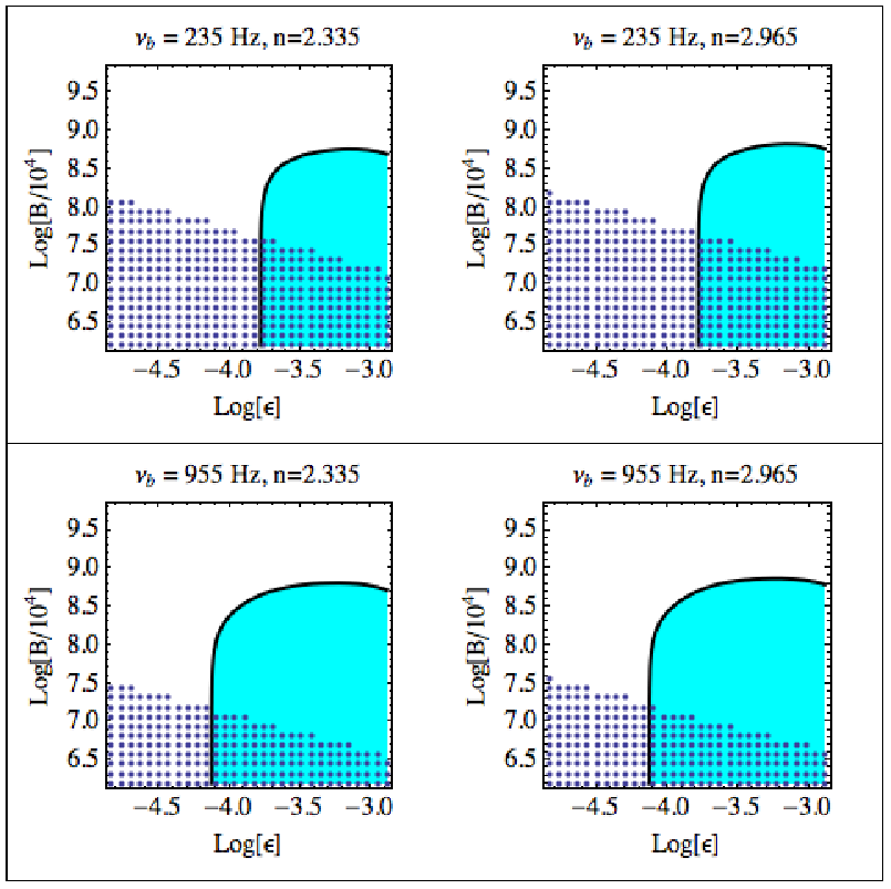
Unfortunately, the number of search templates required to cover the shaded region in Figure 4 is prohibitively large, as discussed in Section 6.2. Figure 5 shows both sensitivity and computational cost. Regions in which the search is sensitive (i.e. ) for given and are shaded in cyan. Overplotted as dark blue dots are the central coordinates of our grid boxes with . The panels correspond to a range of birth frequencies, , and are grouped in pairs: (left panel in pair) and (right panel in pair). The top pair shows the sensitivity and computational cost for Hz, whereas the bottom pair corresponds to Hz (bottom right).
Figure 5 shows that the search sensitivity increases with and , and decreases with . On the other hand, the computational efficiency of the search decreases with and , and increases with . Even so, there is substantial overlap between the regions in which the search is sensitive and the regions which are computationally permissible. We note that as each individual dot in Figure 5 represents a region in which , it is not feasible to search over all the dotted areas, as this would mean . Therefore, when implementing the search, we will choose an appropriate range of parameters such that , using Figure 5 as a guide.
| (kHz) | ( G) | |
|---|---|---|
| 0.19–0.28 | 2.0 | |
| 0.28–0.55 | ||
| 0.55–1.00 |
Table 1 summarises the approximate range of , , and in which the two regions in Figure 5 overlap. If the pulsar in SNR 1987A was born with a frequency between 0.19 kHz and 0.28 kHz, the search is sensitive to and G. This range narrows as increases; for birth frequencies between 0.55 kHz and 1.00 kHz, the search is sensitive to and G. We note that these estimates, derived from the limits on and , assume the standard values for the neutron star mass and radius, and km. It is possible that SNR 1987A contains a low-mass neutron star with (Imshenik, 1992), in which case the limit on the ellipticity, for kHz, would be .
We now comment briefly on the relevance of these limits. The range of listed in Table 1 is within the expected theoretical range discussed in Section 2 (Michel, 1994; Ögelman & Alpar, 2004). The range of listed in Table 1, however, is larger than the maximum ellipticity sustainable by the unmagnetized neutron star crust for many equations of state. For example, conventional neutron stars are expected to support , while hybrid quark-baryon or meson-condensate stars can support (Ushomirsky et al., 2000; Owen, 2005; Horowitz & Kadau, 2009). However, some exotic models do allow for larger ellipticities. Solid strange quark stars are predicted to be able to sustain (Owen, 2005). For low-mass neutron stars, the limit is (Imshenik, 1992; Horowitz, 2010). We note also that these limits apply only to elastically supported deformations; magnetically supported deformations can be larger (Melatos, 2007; Akgün & Wasserman, 2008; Haskell, 2008). Therefore, even placing the relatively large upper limit of on the putative neutron star in SNR 1987A will be useful to some degree in constraining its mass and/or equation of state.
7 Conclusion
In this paper, we describe the steps taken to quantify the astrophysical significance of a cross-correlation search for the supernova remnant SNR 1987A in LIGO S5 data.
- •
We estimate the theoretical sensitivity of the cross-correlation search, and compare it to the conservative, age-based, wave strain estimate. In the frequency band 75 Hz 450 Hz, the age-based estimate lies above the detection threshold.
- •
We introduce an alternative to the Taylor expansion model of the gravitational wave phase based on a set of four astrophysical search parameters (). The new phase model renders a search for a neutron star like SNR 1987A with a high spin-down rate computationally feasible.
- •
To estimate the optimal template spacing for the search, we calculate the semi-coherent phase metric corresponding to this astrophysical model.
- •
We place detection limits on and for a range of birth spin frequencies, 0.1 kHz 1.2 kHz.
With the required template spacing and current computational capabilities discussed in Section 6.2, we will be able to search up to approximately templates. In the event of a non-detection, considering the parameter range discussed in this paper and assuming the standard neutron star mass and radius, we expect to place the following limits on the pulsar’s ellipticity and magnetic field: , G. The search is also expected to be sensitive to electromagnetic braking indices . Its greatest weakness remains that it assumes to be constant throughout the semi-coherent integration. Constant is the simplest possible astrophysical scenario, and it certainly deserves to be considered in its own right, in view of the overwhelming computational cost of a variable- search. Nevertheless, it is vital to recognize that the constant- hypothesis covers a small fraction of the astrophysical parameter space.
A search using gravitational wave data is anticipated to begin soon and would be the first application of the cross-correlation method to a continuous wave search.
Acknowledgements
CC acknowledges the support of an Australian Postgraduate Award and the Albert Shimmins Memorial Fund. JTW acknowledges the support of NSF grant PHY-0855494, the College of Science at Rochester Institute of Technology, and the German Aerospace Center (DLR). This paper has been designated LIGO Document No. LIGO-P1000089-v3.
Appendix A: Calculation of the coherent metric
This appendix details the calculation of the diagonal terms of the coherent metric, (29). We start by evaluating the frequency at time , by assuming that is a simple sum of separate, independent contributions from gravitational-wave and electromagnetic spin down:
| (43) | |||||
| (44) |
Here, and are constants which satisfy , and the search parameters and are defined at a reference time . Recall that is normalised by , which we set to 1 Hz and do not write down, for simplicity. The first term in (44) follows from the first integral in (43) by assuming . The second term in (44) follows from the second integral in (43) by assuming . Needless to say, the exact solution for follows from solving (25) self-consistently for , but this is too difficult to solve analytically. As the phase metric calculation is useful only in an analytic form, we adopt the approximation in (43).
The phase at time is given by,
| (46) | |||||
Appendix B: Semi-coherent metric
Appendix C: Analytic accuracy estimates for the astrophysical phase model
In this appendix, we motivate (30)–(33) physically by calculating the phase error in two special cases: (i) pure gravitational-wave spin down, and (ii) pure electromagnetic spin down. In the gravitational wave case, (25) reduces to
| (62) | |||||
| (63) |
where we take Hz for simplicity and . The gravitational wave phase at is then
| (64) | |||||
| (65) |
There are two regimes to be considered: (i) , and ii) . In terms of the characteristic age
| (66) |
the two regimes correspond to (i) , and (ii) . In the case of SNR 1987A, we have years (in 2006, when the S5 run began) and hr, i.e. regime (ii).
Given small errors and in and , the phase error that accumulates between the template and the signal after a time is
| (67) | |||||
| (68) |
Overall, therefore, the number of templates required scales as regardless of how rapidly the neutron star is spinning down. This scaling matches the conventional Taylor expansion if and suffice to track the signal () but is much more economical if is needed (), which happens for . In the SNR 1987A search, we cover frequencies above 0.1 kHz, so always contributes significantly. Hence the phase model (25) is always preferable.
Now suppose the electromagnetic term dominates. Equation (25) with Hz reduces to
| (69) | |||||
| (70) |
and the gravitational wave phase after a time is
| (71) | |||||
| (72) |
For small errors , and in , and , the phase error between the template at the signal after a time is
| (74) | |||||
Hence in the electromagnetic limit, the phase error due to scales in the same way as in the gravitational wave limit. The phase error due to scales as , and the phase error due to scales as . Overall, the number of templates required scales as . This represents a saving if the second frequency derivative is important which, as shown above, is true for the range of signal frequencies considered in this search.
References
- Abadie et al. (2010a) Abadie J., et al., 2010a, Phys. Rev. D, 81, 102001
- Abadie et al. (2010b) Abadie J., et al., 2010b, arXiv e-prints:gr-qc/1006.2535
- Abadie et al. (2010c) Abadie J., et al., 2010c, ApJ, 715, 1453
- Abadie et al. (2010d) Abadie J., et al., 2010d, arXiv e-prints: gr-qc/1005.4655
- Abbott et al. (2007a) Abbott B., et al., 2007a, ApJ, 659, 918
- Abbott et al. (2007b) Abbott B., et al., 2007b, Phys. Rev. D, 76, 082003
- Abbott et al. (2007c) Abbott B., et al., 2007c, Phys. Rev. D, 76, 042001
- Abbott et al. (2008) Abbott B., et al., 2008, ApJL, 683, L45
- Abbott et al. (2009a) Abbott B., et al., 2009a, Nature, 460, 990
- Abbott et al. (2009b) Abbott B., et al., 2009b, Phys. Rev. D, 80, 042003
- Abbott et al. (2009c) Abbott B., et al., 2009c, Reports on Progress in Physics, 72, 076901
- Abbott et al. (2009d) Abbott B., et al., 2009d, Phys. Rev. D, 79, 122001
- Abbott et al. (2009e) Abbott B., et al., 2009e, Phys. Rev. D, 80, 047101
- Abbott et al. (2009f) Abbott B. P., et al., 2009f, Physical Review Letters, 102, 111102
- Abbott et al. (2010a) Abbott B. P., et al., 2010a, ApJ, 715, 1438
- Abbott et al. (2010b) Abbott B. P., et al., 2010b, ApJ, 713, 671
- Aglietta et al. (1987) Aglietta M., et al., 1987, Europhysics Letters, 3, 1315
- Akgün & Wasserman (2008) Akgün T., Wasserman I., 2008, MNRAS, 383, 1551
- Amaldi et al. (1989) Amaldi E., Bassan M., Coccia E., Bonifazi P., Castellano M. G., 1989, New York Academy Sciences Annals, 571, 561
- Arzoumanian et al. (2002) Arzoumanian Z., Chernoff D. F., Cordes J. M., 2002, ApJ, 568, 289
- Bahcall et al. (1987) Bahcall J. N., Dar A., Piran T., 1987, Nature, 326, 135
- Balasubramanian et al. (1996) Balasubramanian R., Sathyaprakash B. S., Dhurandhar S. V., 1996, Phys. Rev. D, 53, 3033
- Bandiera et al. (1988) Bandiera R., Pacini F., Salvati M., 1988, Nature, 332, 418
- Barkat & Wheeler (1988) Barkat Z., Wheeler J. C., 1988, ApJ, 332, 247
- Bionta et al. (1987) Bionta R. M., Blewitt G., Bratton C. B., Caspere D., Ciocio A., 1987, Physical Review Letters, 58, 1494
- Blandford & Romani (1988) Blandford R. D., Romani R. W., 1988, MNRAS, 234, 57P
- Bonanno et al. (2005) Bonanno A., Urpin V., Belvedere G., 2005, A&A, 440, 199
- Bonazzola & Gourgoulhon (1996) Bonazzola S., Gourgoulhon E., 1996, A&A, 312, 675
- Bondarescu et al. (2009) Bondarescu R., Teukolsky S. A., Wasserman I., 2009, Phys. Rev. D, 79, 104003
- Brady & Creighton (2000) Brady P. R., Creighton T., 2000, Phys. Rev. D, 61, 082001
- Brink et al. (2004) Brink J., Teukolsky S. A., Wasserman I., 2004, Phys. Rev. D, 70, 124017
- Brown & Bildsten (1998) Brown E. F., Bildsten L., 1998, ApJ, 496, 915
- Burrows et al. (2000) Burrows D. N., Michael E., Hwang U., McCray R., Chevalier R. A., Petre R., Garmire G. P., Holt S. S., Nousek J. A., 2000, ApJL, 543, L149
- Cutler (2002) Cutler C., 2002, Phys. Rev. D, 66, 084025
- Dhurandhar et al. (2008) Dhurandhar S., Krishnan B., Mukhopadhyay H., Whelan J. T., 2008, Phys. Rev. D, 77, 082001
- Dickson & Schutz (1995) Dickson C. A., Schutz B. F., 1995, Phys. Rev. D, 51, 2644
- Dotani et al. (1987) Dotani T., Hayashida K., Inoue H., Itoh M., Koyama K., 1987, Nature, 330, 230
- Duncan & Thompson (1992) Duncan R. C., Thompson C., 1992, ApJL, 392, L9
- Faucher-Giguère & Kaspi (2006) Faucher-Giguère C.-A., Kaspi V. M., 2006, ApJ, 643, 332
- Fryer et al. (1999) Fryer C. L., Colgate S. A., Pinto P. A., 1999, ApJ, 511, 885
- Giampanis (2008) Giampanis S., 2008, PhD thesis, University of Rochester
- Gilmozzi et al. (1987) Gilmozzi R., Cassatella A., Clavel J., Fransson C., Gonzalez R., Gry C., Panagia N., Talavera A., Wamsteker W., 1987, Nature, 328, 318
- Graves & et al. (2005) Graves G. J. M., et al. 2005, ApJ, 629, 944
- Haskell (2008) Haskell B., 2008, Classical and Quantum Gravity, 25, 114049
- Haskell et al. (2008) Haskell B., Samuelsson L., Glampedakis K., Andersson N., 2008, MNRAS, 385, 531
- Heger et al. (2003) Heger A., Fryer C. L., Woosley S. E., Langer N., Hartmann D. H., 2003, ApJ, 591, 288
- Hirata et al. (1987) Hirata K., Kajita T., Koshiba M., Nakahata M., Oyama Y., 1987, Physical Review Letters, 58, 1490
- Horowitz (2010) Horowitz C. J., 2010, Phys. Rev. D, 81, 103001
- Horowitz & Kadau (2009) Horowitz C. J., Kadau K., 2009, Physical Review Letters, 102, 191102
- Immler et al. (2007) Immler S., Weiler K., McCray R., eds, 2007, SUPERNOVA 1987A: 20 YEARS AFTER: Supernovae and Gamma-Ray Burste Vol. 937 of American Institute of Physics Conference Series
- Imshenik (1992) Imshenik V. S., 1992, Sov. Astron. Lett., 18, 194
- Inoue et al. (1991) Inoue H., Hayashida K., Itoh M., Kondo H., Mitsuda K., Takeshima T., Yoshida K., Tanaka Y., 1991, Publ. Astron. Soc. Jpn., 43, 213
- Jaranowski et al. (1998) Jaranowski P., Królak A., Schutz B. F., 1998, Phys. Rev. D, 58, 063001
- Manchester (2007) Manchester R. N., 2007, in Immler S., Weiler K., McCray R., eds, Supernova 1987A: 20 Years After: Supernovae and Gamma-Ray Bursters Vol. 937 of American Institute of Physics Conference Series, Searching for a Pulsar in SN1987A. pp 134–143
- Mastrano (2010) Mastrano A., 2010, PhD thesis, UNIVERSITY OF MELBOURNE, AUSTRALIA
- Melatos (1997) Melatos A., 1997, MNRAS, 288, 1049
- Melatos (2000) Melatos A., 2000, MNRAS, 313, 217
- Melatos (2007) Melatos A., 2007, Advances in Space Research, 40, 1472
- Melatos & Payne (2005) Melatos A., Payne D. J. B., 2005, ApJ, 623, 1044
- Michel (1994) Michel F. C., 1994, MNRAS, 267, L4
- Middleditch et al. (2000) Middleditch J., Kristian J. A., Kunkel W. E., Hill K. M., Watson R. D., Lucinio R., Imamura J. N., Steiman-Cameron T. Y., Shearer A., Butler R., Redfern M., Danks A. C., 2000, New Astronomy, 5, 243
- Nakamura (1989) Nakamura T., 1989, Progress of Theoretical Physics, 81, 1006
- Nayyar & Owen (2006) Nayyar M., Owen B. J., 2006, Phys. Rev. D, 73, 084001
- Niebauer et al. (1993) Niebauer T. M., Rüdiger A., Schilling R., Schnupp L., Winkler W., Danzmann K., 1993, Phys. Rev. D, 47, 3106
- Ögelman & Alpar (2004) Ögelman H., Alpar M. A., 2004, ApJL, 603, L33
- Ostriker & Gunn (1969) Ostriker J. P., Gunn J. E., 1969, ApJ, 157, 1395
- Ott et al. (2006) Ott C. D., Burrows A., Thompson T. A., Livne E., Walder R., 2006, ApJS, 164, 130
- Owen (1996) Owen B. J., 1996, Phys. Rev. D, 53, 6749
- Owen (2005) Owen B. J., 2005, Physical Review Letters, 95, 211101
- Owen et al. (1998) Owen B. J., Lindblom L., Cutler C., Schutz B. F., Vecchio A., Andersson N., 1998, Phys. Rev. D, 58, 084020
- Pacini & Salvati (1987) Pacini F., Salvati M., 1987, ApJ, 321, 447
- Palomba (2005) Palomba C., 2005, MNRAS, 359, 1150
- Panagia (1987) Panagia N., 1987, in Danziger I. J., ed., European Southern Observatory Astrophysics Symposia Vol. 26 of European Southern Observatory Astrophysics Symposia, Ultraviolet photometry and the energetics of SN 1987A. pp 55–62
- Panagia (2008) Panagia N., 2008, Chinese Journal of Astronomy and Astrophysics Supplement, 8, 155
- Percival et al. (1995) Percival J. W., Boyd P. T., Biggs J. D., Dolan J. F., Bless R. C., Elliot J. L., Nelson M. J., Robinson E. L., Taylor M. J., van Citters G. W., Wolinski K. G., 1995, ApJ, 446, 832
- Piran & Nakamura (1988) Piran T., Nakamura T., 1988, Progress of Theoretical Physics, 80, 18
- Pletsch (2010) Pletsch H., , 2010, Parameter-space metric of semicoherent searches for continuous gravitational waves, LIGO document LIGO-P1000006-v1, available in http://dcc.ligo.org
- Pletsch & Allen (2009) Pletsch H. J., Allen B., 2009, Physical Review Letters, 103, 181102
- Podsiadlowski & Joss (1989) Podsiadlowski P., Joss P. C., 1989, Nature, 338, 401
- Podsiadlowski et al. (1990) Podsiadlowski P., Joss P. C., Rappaport S., 1990, A&A, 227, L9
- Podsiadlowski et al. (2007) Podsiadlowski P., Morris T. S., Ivanova N., 2007, in Immler S., Weiler K., McCray R., eds, Supernova 1987A: 20 Years After: Supernovae and Gamma-Ray Bursters Vol. 937 of American Institute of Physics Conference Series, The progenitor of SN 1987A. pp 125–133
- Prix (2007) Prix R., 2007, Phys. Rev. D, 75, 023004
- Prix & Whelan (2007) Prix R., Whelan J. T., 2007, Classical and Quantum Gravity, 24, 565
- Reisenegger (2003) Reisenegger A., 2003, arXiv:astro-ph/0307133
- Saio et al. (1988) Saio H., Nomoto K., Kato M., 1988, ApJ, 331, 388
- Santostasi et al. (2003) Santostasi G., Johnson W., Frank J., 2003, ApJ, 586, 1191
- Shternin & Yakovlev (2008) Shternin P. S., Yakovlev D. G., 2008, Astronomy Letters, 34, 675
- Soida et al. (2003) Soida K., Ando M., Kanda N., Tagoshi H., Tatsumi D., Tsubono K., the TAMA Collaboration 2003, Classical and Quantum Gravity, 20, 645
- Sugerman et al. (2005) Sugerman B. E. K., Crotts A. P. S., Kunkel W. E., Heathcote S. R., Lawrence S. S., 2005, ApJ, 627, 888
- Umstäetter et al. (2008) Umstäetter R., Meyer R., Christensen N., 2008, arXiv e-prints: gr-qc/0808.2225
- Umstätter et al. (2004) Umstätter R., Meyer R., Dupuis R. J., Veitch J., Woan G., Christensen N., 2004, Classical and Quantum Gravity, 21, 1655
- Ushomirsky et al. (2000) Ushomirsky G., Cutler C., Bildsten L., 2000, MNRAS, 319, 902
- Vigelius & Melatos (2009a) Vigelius M., Melatos A., 2009a, MNRAS, 395, 1972
- Vigelius & Melatos (2009b) Vigelius M., Melatos A., 2009b, MNRAS, 395, 1985
- Vigelius & Melatos (2010) Vigelius M., Melatos A., 2010, ApJ, 717, 404
- Wette et al. (2008) Wette K., Owen B. J., et al., 2008, Classical and Quantum Gravity, 25, 235011
- Whelan (2006) Whelan J. T., , 2006, Comments on Anisotropic Stochastic Background Searches, Online document. http://www.ligo.caltech.edu/docs/T/T060162-01.pdf
- Whitbeck (2006) Whitbeck D. M., 2006, PhD thesis, Proquest Dissertations And Theses 2006. Section 0176, Part 0606 84 pages; [Ph.D. dissertation].United States – Pennsylvania: The Pennsylvania State University; 2006. Publication Number: AAT 3231915. Source: DAI-B 67/08, Feb 2007
- Woosley (1988) Woosley S. E., 1988, ApJ, 330, 218
- Woosley et al. (2002) Woosley S. E., Heger A., Weaver T. A., 2002, Reviews of Modern Physics, 74, 1015
- Woosley & Weaver (1995) Woosley S. E., Weaver T. A., 1995, ApJS, 101, 181