Robust Estimation through Schoenberg transformations
Robust Estimation of Location through Schoenberg transformations
Abstract
Schoenberg transformations, mapping Euclidean configurations into Euclidean configurations, define in turn a transformed inertia, whose minimization produces robust location estimates. The procedure only depends upon Euclidean distances between observations, and applies equivalently to univariate and multivariate data. The choice of the family of transformations and their parameters defines a flexible location strategy, generalizing -estimators. Two regimes of solutions are identified. Theoretical results on their existence and stability are provided, and illustrated on two data sets.
Keywords: Correspondence Analysis, Euclidean distances, Huber function, Huygens principles, -estimators, Schoenberg transformations, Tukey bisquare
1 Introduction and main result
This paper investigates the properties of presumably new location estimates, defined through Schoenberg transformations, which map initial Euclidean distances into new Euclidean distances (Schoenberg 1938; Bavaud 2011).
Specifically, consider an univariate sample with weights . The weighted mean minimizes , and the weighted median minimizes . This paper introduces and studies a family of centroids , suitable for any dimension, generalizing the previous well-known basic estimates. The centroids are defined as the averages minimizing the transformed inertia
| (1) |
where is a squared Euclidean distance and a Schoenberg transformation (see section 2.2).
The profile generating minimizers turns out to satisfy
| (2) |
This pair of identities defines an iterative scheme, depending on the distances between observations only, and converging in general towards a local minimum of (1). The term downweights observations distant from the centroid , which behaves as a multidimensional robust estimate of location, comparable to the -estimates in the one-dimensional case.
Section 2 defines the main ingredients and presents general results, in particular the existence of two regimes of solutions. Section 3 shows the connection with the theory of -estimates in one dimension, illustrated by the copper concentration data in Section 4. Section 5 illustrates the multidimensional case by means of the chi-square distances occurring in correspondence analysis.
2 Definitions and general results
Data are characterized by the matrix of dissimilarities between observations , together with their weights with . We assume the dissimilarities to be squared Euclidean, that is of the form where the coordinates , unique up to a translation and a rotation, can be recovered by MDS (see e.g. Mardia et al. 1979; Borg and Groenen 1997; Bavaud 2011; and references therein), in a space of dimension .
Here and in the sequel, we assume that observations are distinct, that is for . That is, possibly identical initial observations should be first aggregated into a single observation of weight .
2.1 Huygens principles
The inertia , measuring the dispersion of the weighted configuration, expresses as in either equivalent two forms (Huygens weak principle)
| (3) |
where and . Also (Huygens strong principle)
| (4) |
Consider another distribution or profile with , with associated centroid . Substituting to in (4) yields the second identity in (2). Also, , which shows in (1) to be minimum for in the identity case - an elementary result.
2.2 Schoenberg transformations
A Schoenberg transformation is a componentwise mapping with the property that if represents a squared Euclidean distance between observations and , so does (irrespectively of the dimension ).
The class of all Schoenberg transformations has been investigated and determined by Schoenberg (1938, Theorem 6 p. 828; Bavaud 2011):
Theorem 2.1 (Schoenberg 1938)
The function is a Schoenberg transformation iff of the form
| (5) |
where is a non-negative measure on such that .
Equivalently, is a Schoenberg transformation iff it is smooth, with , and for all
The second part is a consequence of Bernstein theorem on completely monotonic functions. In particular, a Schoenberg transformation is increasing, concave, and zero at the origin. Examples are provided by (Bavaud 2011):
A transformation is said to be rectifiable if , that is iff . By (5), rectifiable transformations obtain as mixtures of , which tends to the identity for .
A transformation is said to be bounded if , that is iff . By (5), bounded transformations obtain as mixtures of , which tends for to the discrete metric , attributing a unit dissimilarity between distinct observations.
The power transformation is not rectifiable nor bounded; the exponential transform is rectifiable and bounded; the logarithmic transformation is rectifiable but not bounded.
2.3 High-dimensional embedding and strain
To the matrix of transformed squared distances correspond, by MDS, new coordinates , unique up to a rotation and translation. Thus, a Schoenberg transformation induces a mapping or embedding of the original coordinates into the transformed coordinates, similar to the high-dimensional embeddings of Machine Learning (Bavaud 2011).
Let denote a position in the the transformed space, and define
On one hand,
in view of Section 2.1. On the other hand, minimizing the transformed inertia amounts in minimizing under the additional constraint for some . The importance of that constraint, reflecting the non-linearity of the embedding , can be measured by the strain , obeying by construction.
2.4 Behavior of minima
Two types of minima exist: distributed minima, where the identities (2) hold, and is strictly positive at each observation; and concentrated minima, where is concentrated on some observation , thus making . The latter case holds iff the quantity is infinite.
Theorem 2.2
1a) when the transformation is rectifiable, a minimizer of necessarily satisfies the identities in (2) (distributed case)
1b) the minimizer also necessarily satisfies the stability condition
| (10) |
where is another point and the angle between the vectors and . In particular, is stable if
| (11) |
2) when the transformation is not rectifiable, a minimizer either behaves as in the distributed case 1), or in a concentrated way, with support concentrated on a single observation .
Proof
See the appendix for a proof of 1a) and 1b). To prove 2), note that equation (2) is not justified anymore iff for some . As is always finite for , then, necessarily, and (non-rectifiable transformation). The observations being distinct, this situation depicts a centroid concentrated on an unique (concentrated case). In particular, this regime necessarily holds whenever the distributed stability condition (10) is violated.
The concentration of the minimizing profile can be measured by its entropy , where iff the profile is concentrated.
3 The univariate case
In one dimension, minimizing yields
The odd function defined for as
| (12) |
is known as the “-function” in the theory of -estimators (e.g. Huber 1964, Hampel et al. 1986, Maronna et al. 2006 and references therein). It is fair to add that the iterative scheme (2) also generalizes the -estimation of location proposed by Tukey (1977), itself identified as a particular case of the -estimation (Hampel et al. 1986 p.116).
The sign of the derivative
| (13) |
governs the stability of the -estimate, in accordance with Theorem 2.2 1b), where conditions (10) and (11) now coincide in view of in one dimension.
3.1 Power transformation
The power transformation with is not rectifiable nor bounded. It exhibits both regimes, namely, distributed solutions for and concentrated ones for , as demonstrated by the study of the sign of (see figure 3).
3.2 Rectifiable transformations
Transformations satisfying can be written as
| (14) |
where is a (squared) characteristic length, and is immaterial for our purpose. Such are the exponential and logarithmic transformations of Section 2.2, as well as the Tukey and Huber transformations
As a matter of fact, the -functions associated to those transformations can be shown to respectively yield the so-called Tukey bisquare and the Huber function, familiar in the theory of -estimates, whence their names. The derivatives of the Tukey and the Huber transformations follow the pattern of Theorem 2.1, except at the value , presenting a discontinuity in the third, respectively second-order derivative.
Theorem 3.1 (rectifiable transformations; proof in the appendix)
There exists a finite characteristic length granting the uniqueness of the minimizer for , with .
3.3 Bounded transformations
Bounded transformations can be written as
| (22) |
Such is the case of the discrete metric , attributing a unit dissimilarity between distinct observations. The transformed inertia reads , and attains its minimum values when , thus generating concentrated solutions only.
This behavior is emblematic of bounded transformations in general (rectifiable or not), which tend towards the discrete metric in the limit (Section 2.2). Hence, by continuity, minima emerge in the limit of small characteristic length:
Theorem 3.2 (bounded transformations)
There exists a finite characteristic length granting the existence of minima, for , each being located near an observation .
4 Illustration: copper concentrations data
Consider the dataset chem, available in the R library MASS (Venables and Ripley 2002) consisting of copper concentrations in wholemeal flour (Abbey, 1988), with sorted values
2.20 2.20 2.40 2.40 2.50 2.70 2.80 2.90 3.03 3.03 3.10 3.37
3.40 3.40 3.40 3.50 3.60 3.70 3.70 3.70 3.70 3.77 5.28 28.95Ê
Ties occur twice ( = 2.20, 2.40, 3.03), three times ( = 3.40) or four times ( = 3.70), and must preliminarily aggregated, resulting in a sample of observations with varying weights.
Figure 1 plots the functions resulting form the exponential and the power transform, for varying parameters. It illustrates the gradual emergence of minima from the mean , in accordance to Section 3. In the power case at the transition value , the minimum is attained at the median interval (second plot of figure 1, right).
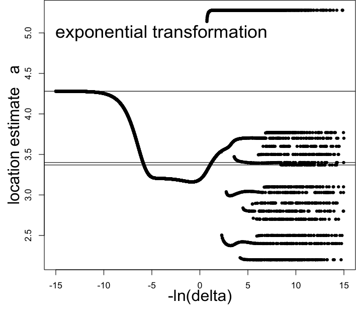
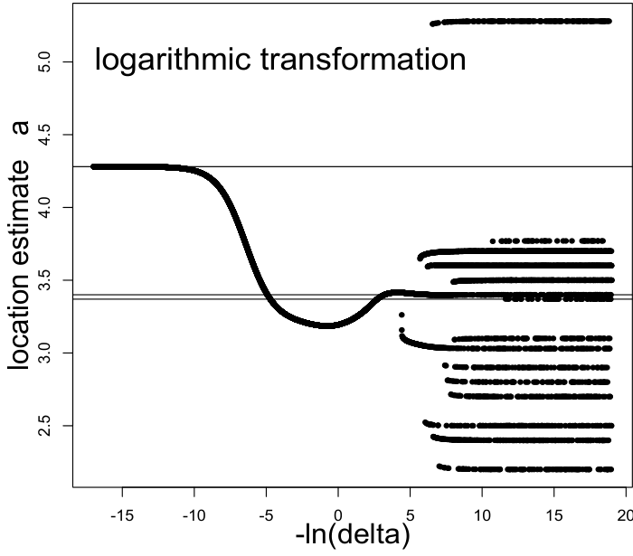
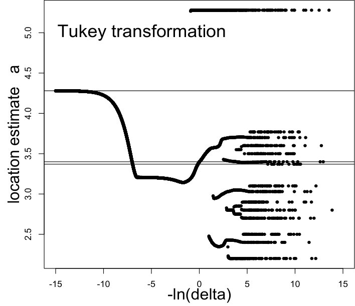
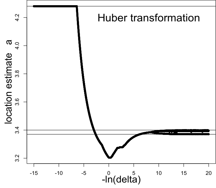
Figures 2 and 3 exhibit the values resulting from the iteration of equations (2), for various transformations and various range of parameters, starting with an initial value drawn as (which de facto excludes the solutions around , for readability sake).
The rectifiable transformations (Figure 2) yield distributed solutions (in accordance with 1a) and 1b) of Theorem 2.2), unique for large characteristic length (Theorem 3.1), and, in the case of bounded exponential and Tukey transformations, “quasi-concentrated” for large characteristic length (Theorem 3.2).
By contrast, the power transformation (Figure 3) exhibits a phase transition at (the median) between distributed and concentrated regimes (Section 3.1 and Theorem 2.2). The value of the strain can be shown to converge for to , where is the weight of the observation on which the minimum is concentrated; it ranges from (ties occurring four times) to (no ties).
As expected, the value of the entropy is zero in the concentrated regime. Figure 3 bottom right demonstrates its deceptive behavior when the aggregation of ties is neglected. Also, the entropy dramatically decreases when the distributed solution crosses the sample values.


5 The multivariate case
The robust estimation scheme (2) depends on the distance matrix only, and not on the coordinates nor on their dimension. The multivariate nature of data is then of little concern, in contrast to early attempts of generalizing -estimates (such as the “peeling” or the “iterative trimming” schemes cited in Maronna (1976)). Rather, the success of the multidimensional implementation boils down to the ability to define an univocal squared Euclidean distance for multidimensional data. This is typically the case for the chi-square metric of Correspondence Analysis (CA) (Benzécri 1973, Greenacre 1984), illustrated below.
5.1 Illustration: scientific collaborations of India
Consider the contingency table giving the number of scientific publications (1993-2000) co-authored by India and foreign countries (rows), sorted by disciplines (columns) (Anuradha and Urs 2007). The natural distance between countries is the chi-square distance
| (23) |
where the dot symbol sums over all values of the corresponding index. The associated inertia is, up to the total count, the chi-square measure of rows-columns dependence; the determination of its low-dimensional projection defines the well-known Correspondence Analysis procedure.
CA extracts uncorrelated factorial coordinates such that , each dimension accounting for a proportion of explained inertia, decreasing with . Figure 4 left exhibits the countries coordinates in the first and second dimensions. The size of the circles depicts the countries weights, maximum for the the USA, whose coordinates are also the closest to the origin.

Figure 4 right depicts the plane trajectories, under various transformations in the distributed regime, of the centroid projections for , where is the profile resulting from (2). All trajectories, diverse in shape and small in amplitude, lead from the the mean at the origin (circle) to the coordinates of the USA (triangle).
6 Conclusion
Classical multidimensional scaling extracts the coordinates of the objects, uniformly weighted or not, from their Euclidean inter-distances only. In the same circumstances, this paper proposes a class of robust location estimates, based upon a Schoenberg transformation of distances, and exhibiting a wide-ranging behavior. Further studies on their sensitivity, breakdown points and the like should presumably help addressing the question “which transformation should be used in which context”, left aside in the present set-up.
Additional guidance is also expected from a probabilistic point of view, deliberately avoided as well in this paper. Manifestly, Schoneberg transformations can serve in generating new densities: typically, replacing the distances in an univariate normal distribution by their square root produces an exponential distribution, which constitutes, in the spirit of Section 2.3, a normal distribution in some higher-dimensional embedded space. In that context, maximum likelihood considerations should also help in selecting a suitable family of transformations - whose Euclidean nature constitutes a favorable circumstance, regarding their tractabillity.
References
- (1) Abbey, S. (1988) Robust measures and the estimator limit. Geostandards Newsletter 12, 241–248
- (2) Anuradha, K.T. and Urs, S.R. (2007) Bibliometric indicators of Indian research collaboration patterns: A correspondence analysis. Scientometrics 71, 179–189
- (3) Bavaud, F. (2011) On the Schoenberg Transformations in Data Analysis: Theory and Illustrations . To appear in the Journal of Classification
- (4) Benzécri, J.P. and Collaborators (1973) L’analyse des données: II L’analyse des correspondances. Bordas, Paris
- (5) Borg, I., Groenen, P.J.F. (1997) Modern multidimensional scaling: theory and applications. Springer
- (6) Greenacre, M. J. (1984) Theory and Applications of Correspondence Analysis. Academic Press
- (7) Hampel, F.R., Elvezio M. Ronchetti, E.M., Rousseeuw, P.J., and Stahel, W.A. (1986) Robust Statistics - The Approach Based on Influence Functions, Wiley
- (8) Huber, P.J. (1964) Robust Estimation of a Location Parameter. The Annals of Mathematical Statistics 35, 73–101
- (9) Mardia, K.V., Kent, J.T., Bibby, J.M. (1979) Multivariate analysis. Academic Press
- (10) Maronna, R.A., (1976) Robust -Estimators of Multivariate Location and Scatter. The Annals of Statistics 4, 51–67
- (11) Maronna, R.A., Martin, D.R., Yohai, V. (2006) Robust Statistics - Theory and Methods. Wiley
- (12) Schoenberg, I. J. (1938) Metric Spaces and Positive Definite Functions. Transactions of the American Mathematical Society 44, 522–536
- (13) Tukey, J.W. (1977) Exploratory data analysis, Addison-Wesley
- (14) Venables, W.N. and Ripley, B.D. (2002) Modern applied statistics with S. Springer
7 Appendix
Proof (of Theorem 2.2)
The derivative of a rectifiable transform is bounded. Setting to zero the derivative of with respect to the -th component of the centroid yields
which is the first identity in (2), the second one resulting from the strong Huygens principle of section 2.1. This solution is a minimum if, for all
Setting yields , proving (10). Equation (11) follows form and .
An alternative, less direct proof also obtains by considering perturbing the profile elements rather than the centroid components . The second identity in (2) yields
and hence the minimum condition
which, by comparison to the identity , yields the first identity in (2). Further derivating with respect to yields together with (2) the stability condition
| (24) | |||||
where is an admissible infinitesimal variation of the profile, that is of the form where is another profile. But (e.g. Bavaud 2011) and
by the cosine formula.
Proof (of Theorem 3.1)
By hypothesis, . From (5),
implying by dominated convergence. Hence , and, by continuity for small enough, or equivalently for large enough. As a consequence, the stability condition (11) of Theorem (2.2) holds irrespectively of the value of , that is is convex for large enough, and thus possesses an unique minimum. The latter tends to in the limit , in view of .