Interference of Light in Michelson–Morley Interferometer: A Quantum Optical Approach
Abstract
We investigate how the temporal coherence interference properties of light in a Michelson-Morley interferometer (MMI), using only a single-photon detector, can be understood in a quantum-optics framework in a straightforward and pedagogical manner. For this purpose we make use of elementary quantum field theory and Glaubers theory for photon detection in order to calculate the expected interference pattern in the MMI. If a thermal reference source is used in the MMI local oscillator port in combination with a thermal source in the signal port, the interference pattern revealed by such an intensity measurement shows a distinctive dependence on the differences in the temperature of the two sources. The MMI can therefore be used in order to perform temperature measurements. A related method was actually used to carry out high precision measurements of the cosmic micro-wave background radiation on board of the COBE satellite. The theoretical framework allows us to consider any initial quantum state. The interference of single photons as a tool to determine the peak angular-frequency of a one-photon pulse interfering with a single-photon reference pulse is, e.g., considered. A similar consideration for laser pulses, in terms of coherent states, leads to a different response in the detector. The MMI experimental setup is therefore in a sense an example of an optical device where one can exhibit the difference between classical and quantum-mechanical light using only intensity measurements.
Keywords:
quantum opticspacs
03.65.-w,42.50.-p,05.70.-a,07.60.Ly, 07.87.+vI Introduction
In 2006 G. Smooth and J. Mather shared the Nobel Prize in Physics ”for their discovery of the black-body form and anisotropy of the cosmic micro-wave background radiation (CMB)” [1]. These exciting discoveries were a breakthrough in modern cosmology by the CMB anisotropy and the strong validation of the black body spectrum as predicted by the Big Bang theory. The discovery of the black body form of the CMB spectrum and the high precision measurement of the CMB temperature (see e.g. Ref.[2] ) relied heavily on the so called Far Infrared Absolute Spectrophotometer (FIRAS) [3] on board the Cosmic Background Explorer (COBE) [4, 5]. In short the FIRAS is a Michelson–Morley interferometer enabling a comparison of the interference patterns between an observed source and a reference source on-board the COBE satellite.
In this paper we will make use of Glaubers theory for photon detection [6, 7] (for a guide to the early literature see e.g. Refs.[8] and for text-book accounts see e.g. Refs.[9, 10, 11]) together with elementary quantum mechanics to show how the principles of the FIRAS can be understood in a quantum-optics framework.
In Section we II recapitulate the principles of Glaubers photon detection theory
and the transformation properties of a quantum field in a beam-splitter (see e.g. Refs.[12, 13, 14]). The Glauber theory of optical coherence is by now well established and plays a central role in fundamental studies of quantum interference effects of photon quantum states (see e.g. Refs.[15, 16, 17]). In Section III we consider temporal interference effects in
the Michelson–Morley interferometer for pure quantum states like single-photon states as well as classical states corresponding to coherent states (see e.g. Refs.[8]).
In Section IV we explain the principles of interference of thermal light in
the Michelson–Morley interferometer by using only
vacuum as the reference source and reproduce known expressions and, in Section V, we consider the full system with an observed thermal source combined with
a thermal reference source. With the results obtained we then explain the basic principle of FIRAS
and how it was used as a high precision thermometer. In Section VI we, finally, give some concluding remarks.
Our presentation extends a recent presentation by Donges [18] and illustrates, e.g., that a quantum-mechanical treatment directly leads to the concept of a thermal coherence length without explicitly making use of classical results like the Wiener-Kintchine theorem as in Ref.[18].
II The Michelson-Morley interferometer
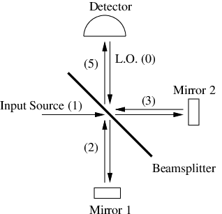
We consider the Michelson-Morley interferometer (MMI) as illustrated in Fig.1, where the so called temporal coherence properties of the radiation field is probed (for an early account see e.g. Ref.[19]). In order to understand the appearance of interference effects in the MMI, we first discuss the separate parts of the MMI before we consider the full setup with the presence of a reference beam.
II.1 Glaubers theory of photon detection
Let us first outline a simple, but not unrealistic, model of a photon detector situated at the space-time point . In this simplified model of a photon detection process [6, 7], the detection of the photon is described by an annihilation of a photon at the detector which modifies the initial state as follows:
| (1) |
The observable electric field operator is described in terms of a suitable normal mode expansion, indexed by mode the number , as a superposition of positive and negative angular-frequency contributions:
| (2) |
where () contains an annihilation (creation) operator for a photon with mode number . According to the basic Born rule in quantum mechanics, the probability to detect the system in a final state , after the one-photon absorption process, is then proportional to . Since the exact details of the final states are, in general, unknown we sum over all possible final states . In general, we also have to consider not only a pure initial quantum state but also a quantum state as described by a density matrix. This leads to a description of the observed intensity which we write in form
| (3) |
where is the density matrix describing the initial state, and where use have be made of the completeness of all possible final states, i.e. . Since we will not be interested in the absolute normalization of the observed intensity , we can neglect normalization constants that may enter into . It is a remarkable fact that an analysis of single-photon interference in a Young interferometer using such a quantum-mechanical description of the photon detection process is fairly recent in the history physics [20] as well as a proper experimental investigation of single-photon interference [22, 21].
For reasons of clarity, we will now consider a normal mode expansion of the electro-magnetic field observable in terms of plane waves, i.e. in terms of a mode sum over wave-vectors and polarization-vector labels , i.e. we have for its positive angular-frequency part that
| (4) |
Here and is a suitable retarded time parameter which will be given in terms of the time-of-flight, given the optical paths in the MMI setup. If the direction of the light beams considered are well-defined, the dependence of the detector position can be neglected in the expression for . In general spatial modulations of the measured intensity are expected [23, 24]. A theoretical analysis of such effects along lines as discussed in the literature (see e.g. Refs. [25, 26]) will, however, not enlighten the issues we are addressing in the present paper. is a quantization volume that will be allowed to be arbitrarily large at an appropriate late stage of our calculations. is the annihilation operator describing the detected light and denotes the unit polarization vector of the normal mode considered.
Since, in the end, the dependence of normalization constants will be irrelevant, and since we will only consider polarization-independent optical devices, we make use of a scalar notation. We therefore suppress the wave-vector and polarization labels and with we write , such that in terms of a discrete Kronecker delta . We also make use of the following convenient notation [10] for the positive angular-frequency part of the electric field at the position of the detector at time
| (5) |
Here now denotes an optical phase which explicitly takes the source-detection retardation time into account by the time-delay , which will be evaluated for the MMI-setup below. If the detector time enters explicitly into the detection intensity Eq.(3), we will perform a time-average which corresponds to a finite detector time-resolution window. The corresponding time-average of the observed intensity will be denoted by , i.e.
| (6) |
where the time of integration, as e.g. the time during which an actual measurement proceeds, is chosen to be sufficiently large in comparison with any reciprocal bandwidth of the initial quantum states considered. The time-averaged observed intensity will in general, as we will see explicitly below, be a function of a time-delay depending on the actual experimental set-up.
For a finite quantization volume , can be regarded to be discrete and, in the infinite volume limit, we make use of the rule that , where is the number of space-dimensions. We will neglect the dependence of transverse dimensions of very collimated normal modes and assume that . When appropriate we will, however, also consider in order to compare with related results in the literature [18, 19]. Our main results will, however, not be very sensitive to the choice of .
Using the same notation as above, a one-photon quantum state , with an angular-frequency distribution given by , is then given by
| (7) |
where denotes a one-photon state with angular-frequency , normalized according to , and where denotes the vacuum state. We also make use of the notation . The state above is an eigenstate of the number operator , i.e. a Fock state, with, of course, an eigenvalue corresponding to one particle present. Normalization of the state for therefore corresponds to
| (8) |
in the large-volume limit. In order to make our presentation quantitative we will, for reasons of simplicity, consider real-valued one-photon angular-frequency distributions such that
| (9) |
with a mean angular-frequency and width and where the normalization constant is given by
| (10) |
in terms of an error function. This choice of frequency distribution makes it possible to actually carry out all relevant expressions analytically. In obtaining the properly normalized expression Eq.(9) we keep . It may, however, sometimes be possible to extend the range of angular frequencies to arbitrarily negative values in Eq.(8), so that , with an exponential small error, which makes some of the expressions as given below more tractable and transparent. With our choice of beam parameters below it turns out that such an approximation plays only a minor role with regard to actual numerical evaluations.
Conventional coherent states , as expressed in terms of the one-photon distribution , can then be obtained using a multi-mode displacement operator (see e.g. Refs.[8]), i.e.
| (11) |
such that
| (12) |
and hence
| (13) |
II.2 Transformation in the beam-splitter
Next, we consider a beam-splitter with frequency independent transmittance and reflectance . If we assume a prefect beam-splitter, where all light is either reflected or transmitted, we have . The input annihilation operators and of the beam-splitter will then transform according to (see e.g. Refs.[12, 13, 14])
| (14) |
where are the L.O. and signal port mode annihilation operators, and the output annihilation mode operators corresponding to the transmitted and reflected modes, respectively. The –phase-shift between the transmitted and reflected part, described by the complex numbers in Eq.(14) will play and important role below as is also the case in the famous Hong-Ou-Mandel two-photon correlation experiment [27] and related investigations (see e.g. Ref. [28, 29, 30]).

A light beam arriving at the beam-splitter after being reflected in the mirrors and will, in general, be phase shifted, i.e. expressed in terms of mode operators this process corresponds to the time-of-flight replacement
| (15) |
due to difference in optical path lengths with in terms of time-delays and . The reflections at the mirrors in the MMI setup will also introduce a phase-shift of , but this is equal for the two light beams and we can therefore be neglected all together. A light beam passing through the beam-splitter after reflection at the mirrors will, again, transform according to Eq.(14) and we therefore, finally, obtain an expression for the mode operator describing incident light on the photon detector, i.e.
| (16) |
The positive angular-frequency part of the electro-magnetic field operator, , at the position of the detector as given in Eq.(5), will now be expressed in terms of . For reasons of clarity we will consider a beam splitter, i.e. we make the choice , and therefore the corresponding electro-magnetic field operator to be used in Glaubers theory of photon detection, is given by
| (17) |
III Interference of Fock States and Coherent States
Let us now specifically consider the following initial Fock state
| (18) |
for the signal and the local port with one-photon angular-frequency distributions according to Eq.(9) with the same spectral widths but with for the signal port and or for the local oscillator port. We then see that
| (19) |
where we have made use of the fact that , which now defines the optical time-delay . The probability for the detection of one photon will according to Glaubers theory of photon detection, as we have mentioned above, be proportional to the absolute modulus square of the probability amplitude , i.e. to . A time-average over the time according to Eq.(6) with leads to a Kronecker delta and therefore makes any double-sum over frequencies into a single-sum. In the large-volume limit and for , we then obtain
| (20) |
If then, within a good numerical approximation, we can first replace the linear dependence in Eq.(20) with and in front of the corresponding angular-frequency distributions, and then extend the integration to include arbitrarily negative angular-frequencies. One then finds that
| (21) |
where the interference effects are exponentially sensitive to the spectral width of the single-photon angular-distributions similar to the spectral width dependence in the famous Hong-Ou-Mandel two-photon experiment [27]. The asymptotic value of is given by . In Fig.2 we exhibit according to Eq.(20) with the choice as in Eq.(18). It is now clear that with a given reference distribution of the local oscillator one can, e.g., infer the common spectral width of the single-photon sources as well as the corresponding angular-frequency . A related experimental situation is discussed in Ref.[31] for a general one-photon state, i.e. not necessarily a pure quantum state.
In the case of coherent states in the signal and local ports, with one-particle state angular-frequency distributions and as above, Eq.(19) is now modified according to
| (22) |
i.e. Eq.(20) is, for real-valued single-photon distributions and , replaced by
| (23) |
In Fig.3 we exhibit with coherent states generated by the same choice of single-photon states as in Fig.2. The interference is, as in Fig.2, sensitive to the actual angular-frequency distributions. With a given reference distribution of the local oscillator, one can now infer the common spectral width of the coherent state sources as well as the corresponding angular-frequency . By a comparison with Fig.2, we conclude that the MMI setup is sensitive to the actual form of the initial quantum states despite the fact that we are only considering single-photon detection processes.

IV Interference of thermal light in the Michelson-Morley interferometer
IV.1 Thermal light
For the readers convenience, let us first outline a simple and quantum mechanical description of thermal black body radiation at an absolute temperature . Black body radiation is, basically, light with random phases. For a single mode with angular-frequency and if denotes a -photon state, the density matrix describing the thermal light is given by
| (24) |
in terms of the Bose-Einstein distribution
| (25) |
with
The state corresponds to an extreme value of the von Neumann entropy in units of , i.e.
| (26) |
subjected to the constraints (see e.g. Refs.[19, 11])
| (27) |
The random, or chaotic, nature of the quantum state corresponds to a phase-independent Glauber-Sudarshan -representation (see e.g. Refs.[32, 33, 34, 35]) in terms of a coherent state, i.e.
| (28) |
using a single-mode coherent state . For thermal light one finds that
| (29) |
which obeys the normalization condition
| (30) |
as well as
| (31) |
A multi-mode system at thermal equilibrium is then described in terms of a tensor product , where we have performed the replacement in Eqs.(28) and (29). The Glauber-Sudarshan -representation for the state is now, in particular, useful in our considerations since the response in a single-photon detector can be obtained immediately from the previous results for coherent light using an average procedure.
IV.2 Thermal light in the signal port and vacuum in the local oscillator port
We are now in the position to consider a density matrix describing a system where we have thermal light in the signal port and vacuum in the LO port, i.e. the initial density matrix of the total system is given by
| (32) |
By making use of Eq.(23), with and , and then performing an average over according to Eq.(31), we immediately obtain the result
| (33) |
in space dimensions. In passing, we notice that Eq.(33) is actually valid for any physical quantum state of the form Eq.(32) due to the generality of the Glauber-Sudarshan -representation Eq.(28). The interference effects as exhibited by the MMI setup therefore only depends on the, in general, angular-frequency dependent mean-number and not on other features of the actual quantum state considered. By a straightforward change of integration variables in Eq.(33), and with , we then find that
| (34) |
where can be expressed in terms of gamma and Riemann’s functions, i.e.
| (35) |
Particular values are and . In the case of we, therefore, recover the well-known expression for [19] as also discussed in Ref.[18]. In, e.g., it is actually possible to carry out the relevant integral in the expression Eq.(34) for exactly with the result
| (36) |
Eq.(36) shows that interference effects have a power-law sensitivity for larger . In Fig.4 we show for varying values of in the case with and one infers a characteristic coherence length of thermal light in the MMI of the form
| (37) |
as also discussed in Ref.[18].
V Thermal light in the signal and local ports
As we have seen above, with a vacuum in the LO port and with a signal thermal source the single-photon detection process exhibits an interference pattern. We now investigate what happens if we have thermal light with a temperature in the LO port and thermal light with temperature in the signal port. For this setup the corresponding initial density matrix becomes
| (38) |
By making use of this density matrix as well as the same methods as described in Section IV.2 by performing independent averages over and in Eq.(23) according to Eq.(31), we immediately obtain, in the large-volume limit, the result
| (39) |

Here we notice that the last term in Eq.(23), suitably extended to complex-valued and , averages to zero due to the chaotic nature, i.e. phase-independence, of thermal light according to Eqs.(28) and (29). The relative intensity with respect to zero time-delay has then the form
where and . The integrals in Eq.() can, again, be solved analytically in a fashion similar to the integral in Eq.(34), i.e.
Due to the presence of hyperbolic functions in Eq.(), we observe that approaches its asymptotic value exponentially fast as a function of the time-delay in contrast to the power-law dependence in Eq.(36). It is now of interest to study the behavior of Eq.() when the temperature and of the local oscillator and signal respectively are varied. In Fig.5 we exhibit the interference when is slightly smaller or larger than as a function of the parameter for . The corresponding interference, of course, disappears when the two temperatures are equal. The sensitivity of the interference pattern with regard to the difference in temperatures of the source and the reference temperature, i.e. of the local source, constitutes the basic ingredient of the FIRAS setup. We also observe that the coherence length for this MMI setup is the roughly same as in Section IV.2.

VI Conclusions and Final Remarks
We have seen that the interference of thermal light in the Michelson-Morley interferometer can be described, in a straightforward manner, by making use of Glaubers theory of photon detection and elementary quantum theory of the electro-magnetic field. Furthermore, we have seen the emergence of a natural coherence length of thermal light in the MMI. It may be surprising that non-monochromatic and chaotic light, with random phases, exhibits interference effects but, as we have seen, such an interference is naturally traced out in terms of the normal-mode expansion of the quantized electro-magnetic field (see e.g. the comments in Ref.[36]). The result for thermal light in both the signal and the local oscillator ports shows that the interference pattern is sensitive to the difference in temperature of the two sources. This is the basic principle used by the FIRAS on board the COBE satellite in order to perform high precision measurements of the temperature and the spectrum of the cosmic micro-wave background radiation.
Since we have been considering initial quantum states in terms of a fixed number of photons as well as ”classical” states, corresponding to coherent states with an infinite number of photons present, a quantum-mechanical language is mandatory. The signal and local ports of the MMI setup corresponds to independent input sources. It is, of course, a well-known experimental fact that independent photon sources can give rise to interference effects (see e.g. Refs.[37, 38, 39, 40, 41, 42]). Despite the fact that such interference effects are well established, the interpretation of them can, nevertheless, give rise to interesting issues regarding the very fundamental aspects of the quantum-mechanical world (see e.g. [43]) when considering, in particular, interference effects using single-photon sources.
We have seen that for multi-mode systems the quantum nature of theses independent sources actually effects the nature of the single-photon intensity measurements. We have already mentioned that the angular-frequency distribution of a single photon can be measured using a similar experimental setup as the MMI considered in the present paper [31]. With a vacuum state in the local oscillator port and a signal single-photon angular-frequency distribution of the form considered in Eq.(9), one finds, using Eq.(20), that
| (42) |
We conclude, in view of our considerations, by noticing the characteristic exponential behavior in Eq.(42) for single-photon interference is not necessarily the indication of a Lorentzian angular-frequency distribution as claimed in the literature when, e.g., measuring the photo-luminenscene signal of a single quantum dot [44] or in studies of other interference effects of dissimilar photon sources [45].
Acknowledgments. This research has made use of NASA’s Astrophysics Data System. The research was supported by the Research Council of Norway through grants 170935/V30 and FRINAT-191564, and by NTNU. One of the authors (B.-S.S.) wishes to thank Professor Frederik G. Scholtz for a generous and stimulating hospitality during a joint NITheP and Stias, Stellenbosch (S.A.), workshop in 2009, Professors M. Reid and D. V. Ahluwalia, University of Christchurch, N.Z., J. R. Klauder, University of Florida, Gainesville, U.S.A, P. S. Riseborough, Temple University, U.S.A., and the TH-Division at CERN for hospitality when the present work was in progress.
References
- [1] Nobel Prize Website (http://nobelprize.org/) .
- [2] D. J. Fixsen, , J. C. Mather, ”The spectral results of the Far-Infrared Absolute Spectrophotometer instrument on COBE ”, Ap. J. 581, 817-822 (2002).
- [3] J. C. Mather, D. J. Fixsen, and R. A. Shafer, ”Design for the COBE far-infrared absolute spectrophotometer ” in Society of Photo-Optical Instrumentation Engineers (SPIE) Conference Series, Vol. 2019, SPIE Conference Series, Ed. M. S. Scholl, p.168-179 (1993).
- [4] J. C. Mather, ”The Cosmic Background Explorer (COBE) ”, Optical Engineering, 21, 769-774 (1982).
- [5] J. C. Mather, Section 2.8 in, ”Questions of Modern Cosmology - Galileo’s Legacy”, Eds. M. D’Onofrio and C. Burigana (Springer, Berlin and Heidelberg, 2009).
- [6] R. J. Glauber, ’The Quantum theory of optical coherence”, Phys. Rev. 130, 2529-2539 (1963).
- [7] R. J. Glauber, ”Optical coherence and photon statistics” in: C. DeWitt, A. Blandin, C. C.-T. (Ed.), ”Quantum Optics and Electronics”, Les Houches, p. 621 (Gordan and Breach, New York, 1965).
- [8] J. R. Klauder and B.-S. Skagerstam, ”Coherent States -Applications in Physics and Mathematical Physics” (World Scientific, Singapore 1985 and Beijing 1986); B.-S. Skagerstam, “Coherent States - Some Applications in Quantum Field Theory and Particle Physics ” in “Coherent States: Past, Present, and the Future ”, Eds. D. H. Feng, J. R. Klauder and M. R. Strayer (World Scientific, Singapore, 1994); J. R. Klauder, ”The Current State of Coherent States”, contribution to the 7th ICSSUR Conference, Boston, 2001 (arXiv:quant-ph/0110108v1).
- [9] J. R. Klauder and E. C. G. Sudarshan, ”Fundamentals of Quantum Optics” (W.A. Benjamin, New York, 1968 and Dover Publications, Inc. , New York, 2006).
- [10] L. Mandel and E. Wolf, ”Optical Coherence and Quantum Optics” (Cambridge University Press, Cambridge, UK, 1995).
- [11] M. O. Scully and M. S. Zubairy, ”Quantum Optics” (Cambridge University Press, Cambridge, UK, 1997).
- [12] B. Yurke, S. L. McCall, and J. R. Klauder, ”SU(2) and SU(1,1) interferometers” , Phys. Rev. A 33, 4033-4054 (1986).
- [13] Z. Y. Ou and L. Mandel, ”Derivation of reciprocity relations for a beam splitter from energy balance”, Am. J. Phys. 57, 66-67 (1989).
- [14] R. A. Campos, B. E. A. Saleh, and M. C. Teich, ”Quantum-mechanical lossless beam splitter: SU(2) symmetry and photon statistics”, Phys. Rev. A 40, 1371-1384 (1989).
- [15] L. Mandel, ”Quantum Effects in one-photon and two-photon interference”, Rev. of Mod. Phys. 71, S274-S282 (1999).
- [16] A. Zeilinger, ”Experiment and the foundations of quantum physics”, Rev. of Mod. Phys. 71, S288-S297 (1999).
- [17] A. Zeilinger, G. Weihs, T. Jennewein, and M. Aspelmeyer, ”Happy centenary, photon”, Nature 433, 230-238 (2005) and ibid. 446, 342 (2007).
- [18] A. Donges, ”The coherence length of black-body radiation”, Eur. J. Phys. 19 , 245-249 (1998) .
- [19] L. Mandel and E. Wolf, ”Coherence properties of optical fields”, Rev. of Mod. Phys. 37, 231-287 (1965).
- [20] D. F. Walls, ”A simple field theoretic description of photon interference”, Am. J. Phys. 45, 952-956 (1977).
- [21] A. Aspect and P. Grangier, ”Wave-Particle Duality for Single Photons”, in Hyperfine Interactions 37, 3-18 (1987).
- [22] P. Grangier, G. Roger, and A. Aspect , ”Experimental evidence for a photon anticorrelation effect on a beam splitter: A new light on single-photon interference”, Europhys. Lett. 1, 173-179 (1986).
- [23] T. J. Herzog, J. R. Rarity, H. Weinfurter and A. Zeilinger, ”Frustrated Two-Photon Creation via Interference”, Phys. Rev. Lett. 72, 629-631 (1994).
- [24] G. Scarcelli, A. Valencia, and Y. Shih, ”Experimental study of the momentum correlation of pseudothermal field in photon-counting regime”, Phys. Rev. A 70, 051802(1-4) (2004).
- [25] L. J. Wang, Z. Y. Ou and L. Mandel, ”Induced coherence without induced emission”, Phys. Rev. A44, 4614-4622 (1991) and Section in Ref.[10].
- [26] P. W. Milonni, H. Fern, and A. Zeilinger, ”Theory of two-photon down-conversion in the presence of mirrors”, Phys. Rev. A53, 4556-4566 (1996).
- [27] C. K. Hong, Z. Y. Ou and L. Mandel, ”Measurement of Subpicosecond Time Intervals between Two Photons by Interference”, Phys. Rev. Lett. 59, 2044-2046 (1987).
- [28] Y. H. Shih and C. O. Alley, ”New Type of Einstein-Podolsky-Rosen-Bohm Experiment Using Pairs of Light Quanta Produced by Optical Parametric Down Conversion ”, Phys. Rev. Lett. 61 , 2921-2924 (1988).
- [29] A. M. Steinberg, P. G. Kwiat, and R. Y. Chiao,, ”Measurement of the Single-Photon Tunneling Time ”, Phys. Rev. Lett. 71, 708-711 (1993) and ”Observation of a ”quantum eraser”: A revival of coherence in a two-photon interference experiment ”, Phys. Rev. A45, 7729-7739 (1992).
- [30] D. V. Strekalov, T. B. Pittman, and Y. H. Shih, ”What can we learn about single photons in a two-photon interference experiment ”, Phys. Rev. A57, 567-570 (1997).
- [31] W. Wasliewski, P. Kolenderski, and R. Frankowski, ”Spectral density matrix of a single photon measured”, Phys. Rev. Lett. 99, 123601(1-4) (2007).
- [32] E. C. G. Sudarshan, ”Equivalence of semi-classical and quantum mechanical descriptions of statistical light beams”, Phys. Rev. Lett. 10, 277-279 (1963).
- [33] R. Glauber, ”Coherent and incoherent states of the radiation field”, Phys. Rev. 131, 2766-2788 (1963).
- [34] J. R. Klauder, J. McKenna, and D. G. Currie, ”On “diagonal” coherent-state representations for quantum-mechanical density matrices”, J. Math. Phys. 6, 734-739 (1965); C. L. Metha and E. C. G. Sudarshan, ”Relation between quantum and semi-classical description of optical coherence”, Phys. Rev. 138, B274-B280 (1965) ; J. R. Klauder, ”Improved version of optical equivalence theorem”, Phys. Rev. Lett. 16, 534-536 (1966).
- [35] J. R. Klauder and B.-S. Skagerstam,”Generalized phase-space representations of operators”, J. Phys. A:Math. Theor. 40, 2093-2105 (2007).
- [36] J. Xiong, D.-Z. Cao, F. Huang, H.-G. Li, X.-J. Sun, and K. Wang, ”Experimental Observation of Classical Subwavelength Interference with a Pseudothermal Light Source”, Phys. Rev. Lett. 94, 173601(1-4) (2005).
- [37] G. Magyar, and L. Mandel, ”Interference fringes produced by superposition of two independent laser light beams”, Nature 198, 255-256 (1963).
- [38] R. L. Pfleegor, and L. Mandel, ”Further Experiments on Interference of Independent Photons Beams at Low Light Levels”, JOSA 58, 946-950 (1968).
- [39] L. Mandel, ”Photon interference and correlation effects produced by independent quantum sources”, Phys. Rev. A28, 929-943 (1983).
- [40] H. Paul, ”Interference between independent photons”, Rev. Mod. Phys. 58, 209-231 (1988).
- [41] F. Louradour, F. Reynaud, B. Colombeau, and C. Froehly, ”Interference fringes between two separate lasers”, Am. J. Phys. 61, 242-245 (1993).
- [42] R. K. Kaltenbaek, B. Blauensteiner, M. Ẑukowski, M. Aspelmeyer, and A. Zeilinger, ”Experimental Interference of Independent Photons”, Phys. Rev. Lett 96, 240502(1-4) (2006).
- [43] R. J. Glauber, ”Diracs’s Fameous Dictum on the Interference: One Photon or Two Photons? ”, Am. J. Phys. 63, 12 (1995).
- [44] C. Kammerer, G. Cassabois. C. Voisin, M. Perrin, C. Delalande, Ph. Roussignol, and J. M. Gérard, ”Interferometric correlation spectroscopy in single quantum dots”, App. Phys. Lett. 81, 2737-2739 (2002).
- [45] A. J. Bennet, R. B. Patel, C. A. Nicoll, D. A. Ritchie, and A. J. Shields, ”Interference of dissimilar photon sources”, Nature Physics 5, 715-717 (2009).