On the frequency of oscillations in the pair plasma generated by a strong electric field
Abstract
We study the frequency of the plasma oscillations of electron-positron pairs created by the vacuum polarization in an uniform electric field with strength in the range . Following the approach adopted in [1] we work out one second order ordinary differential equation for a variable related to the velocity from which we can recover the classical plasma oscillation equation when . Thereby, we focus our attention on its evolution in time studying how this oscillation frequency approaches the plasma frequency. The time-scale needed to approach to the plasma frequency and the power spectrum of these oscillations are computed. The characteristic frequency of the power spectrum is determined uniquely from the initial value of the electric field strength. The effects of plasma degeneracy and pair annihilation are discussed.
Keywords:
vacuum polarization, plasma oscillationsPACS
25.75.Dw; 52.27.EpThe electron-positron pair production in a strong electric field is one of the most popular topics in relativistic field theory [2]. It begun with the pioneer works by Sauter [3], Heisenberg and Euler [4], and by Schwinger [5]. This effect acquires particular importance when the electric field strength is larger than the critical value ; such a strong electric field can be reached in astrophysical environments, near quark stars [6]-[7] and neutron stars [8]-[9]. Strong electric fields up to several percents of the critical value will be reached by advanced laser technologies in laboratory experiments [10]-[12], X-ray free electron laser facilities [13], optical high-intensity laser facilities such as Vulcan or the Extreme Light Infrastructure [14], for a recent review see [15]. Electron beam-laser interactions seem also promising in reaching high Lorentz transformed electromagnetic fields capable for multiple pair production [16].
It has been shown that, due to back reaction and screening effects of pairs on external electric fields, positrons and electrons move back and forth coherently with alternating electric field: the so called plasma oscillations. In [1] it was pointed out that this phenomenon occurs also when giving emphasis on the fact that, for overcritical (undercritical) field, a large (small) fraction of the initial electromagnetic energy is converted into the rest mass of pairs, whereas a small (large) fraction is converted into kinetic energy. In [17] the case of spatially inhomogeneous electric field has been considered, the emitted radiation spectrum far from the oscillation region was obtained, presenting a narrow feature.
In this Letter we return to basic equations describing pair creation and plasma oscillations in uniform unbound electric field. We first derive a master equation for a new variable constructed from hydrodynamic velocity, which turns out to be second order ordinary differential equation. This equation is reduced to the classic plasma oscillations equation describing Langmuir waves in the limit of small electric field. The frequency of oscillations is then shown to be almost equal to the plasma frequency, which is strongly time dependent in the case under consideration. Finally, the spectrum of bremsstrahlung radiation is computed following [17] and its characteristic feature is identified as a function of initial value of the electric field strength.
As in [1] we apply an approach based on continuity, energy-momentum conservation and Maxwell equations in order to account for the back reaction of the created pairs focusing on the range .
We assume that electrons and positrons are created at rest in pairs, due to vacuum polarization in uniform electric field [3]-[5], [18]-[20] with the average rate11 1 We use in the following the system of units where , , being the fine structure constant. per unit volume and per unit time
| (1) | |||
| (2) |
where is electromagnetic field tensor, is electron mass.
This formula is derived for uniform constant in time electric field. However, it still can be used for slowly time-varying electric field provided the inverse adiabaticity parameter [19]-[23] is much larger than one,
| (3) |
where is the frequency of oscillations, is dimensionless period of oscillations. Eq. (3) implies that time variation of the electric field is much slower than the rate of pair production. In two limiting cases considered in this Letter, and , we find respectively for the first oscillation , and , whereas for the last one , and .
Following [1] the conservation laws and Maxwell equations written for electrons, positrons and electromagnetic field are
| (4) | ||||
| (5) | ||||
| (6) |
where is the comoving number density of electrons, is energy-momentum tensor of electrons and positrons
| (7) |
where is the total four-current density, is four velocity respectively of positrons and electrons. Electrons and positrons move along the electric field lines in opposite directions.
It has been shown in [1] that in a uniform electric field, from the system (4)-(6), the following system of four coupled ordinary differential equations may be obtained
| (8) | ||||
| (9) | ||||
| (10) | ||||
| (11) |
where is dimensionless number density normalized by the Compton length , is energy density of positrons22 2 Total energy density of electrons and positrons is twice this value., is momentum density of positrons, is electric field strength, and is time, normalized by the Compton time . The rate of pair production is , velocity is and Lorentz factor is .
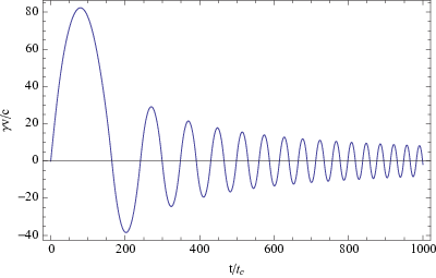


For the system (8)-(11) there exist two integrals (conservation laws)
| (12) | ||||
| (13) |
so the particle energy density vanishes for initial value of the electric field . Combining together the previous two equations, we get for the maximum number density of pairs that can be created
| (14) |
In [1] the system (8)-(11) was reduced to two equations using (12)-(13) and analyzed on the phase plane ().
Notice that the equation of motion of single particle in our approximation is just
| (15) |
where we have defined and introduced a new variable constructed from hydrodynamic velocity as . Then this equation can be combined with (11) to obtain a single master equation
| (16) |
The key point of our treatment is the physical interpretation of Eq. (16) which can be rewritten symbolically as
| (17) |
With constant coefficients Eq. (17) would describe damped harmonic oscillations with frequency and friction . In our case and are time dependent, but Eq. (16) still possesses an oscillating behavior with damping. With our definitions the number density of pairs is
| (18) |
We then identify in (17) as
| (19) |
i.e. the relativistic plasma frequency33 3 The factor is in this formula due to the presence of two charge carriers with the same mass - electrons and positrons. This is different from the classical electron-ion plasma where only electron component oscillates and the corresponding factor is twice smaller..
The function
| (20) |
in Eq. (17) accounts for the rate of pair production (1). It describes the increase of inertia of electron-positron pairs due to increase of their number and causes decrease of the amplitude of oscillations.
For small electric fields Eq. (16) is reduced to classical plasma oscillations equation describing Langmuir waves, since in that case is exponentially suppressed. For this reason we expect that as the amplitude of oscillations of electric field gets smaller the frequency of oscillations tends to the plasma frequency .
In [1] we solved numerically the system of four coupled ordinary differential equations (8)-(11). Now it is possible to solve just one second order differential equation (16) which allows us to study its asymptotic behavior as well.
We solve numerically Eq. (16) with the initial conditions and , corresponding to no pairs in the initial moment, taking for initial electric field strength . Once this equation has been solved, we have the solution for the number density from (18) and for the plasma frequency by means of (19). In Fig. 1 we show the evolution in time of where the amplitude of the oscillations decreases, while its frequency increases with time.
We present the number density of pairs in Fig. 2 for the case as a fraction of the maximum achievable value . In all the cases under interest, this number is asymptotically achieved indicating that the final result of the process will be the complete conversion of the electromagnetic energy density into the rest mass of the pairs. Moreover, looking at Fig. 2 we recover the result obtained in [1]; in fact we can see that after the first oscillation, higher is larger is . This means that the first oscillation gives the leading contribution to the process in which the electromagnetic energy of the field is converted in the rest mass of pairs, with a moderate contribution to their kinetic energy for . The values of the half periods of the first oscillation for each considered case are represented in Fig. 3 by triangles.
We computed the frequency of the -th oscillation as , where is the corresponding half period, calculated considering the time interval between the -th and ()-th subsequent roots of , see Fig. 1.
Notice that is an oscillating function of time, due to the presence of in (19); besides the frequency of these oscillations increases in time. For this reason, in order to get a smooth function we calculated the average of . We use this new function for the plasma frequency to make a comparison with the frequency of oscillations of pairs. In Fig. 4, for the case , the blue area represents the plasma frequency as defined by (19), the yellow curve is its average , while the pairs oscillation frequency is represented by the red curve. For the same initial electric field, in Fig. 5 the trend of the ratio is shown, which indicates that the averaged plasma frequency is achieved asymptotically as expected from (16). Notice that the oscillation frequency is always smaller than since the number density of pairs is constantly increasing with time during each oscillation cycle.
We computed the power spectrum of radiation in the far zone, assuming dipole radiation following [17]. The power spectrum, namely the energy radiated per unit solid angle per frequency interval and per unit volume, is given by
| (21) |
where the amplitude is proportional to the Fourier transform of the electric current time derivative [17]
| (22) |
The electric current is simply related to the new variables by the following expression
| (23) |
From the Fig. 6 it is clear that the main contribution is given by the final and fastest oscillations which last for a longer time. Therefore, the power spectrum shows a peak close to the plasma frequency being reached asymptotically. We can easily estimate the frequency corresponding to this peak combining Eq. (14) with Eq. (19) as
| (24) |
with the corresponding energy MeV.
The energy loss due to the dipole radiation for considered in Fig. 6 for is less than one percent.

Once we know the frequency of the pairs oscillations and the plasma frequency, we obtain their ratio as it is shown in Fig. 5. Besides, we use in order to compute the characteristic time scale needed for the pairs oscillation frequency to reach the plasma frequency. This has been done considering the ratio between and its time derivative; the result of this procedure gives us a numerical function from which we have taken the average. For all the considered cases, this quantity is shown in Fig. 3, from which we understand that the general trend is that larger is the initial electric field, larger will be the starting oscillation frequency.

It is worth noting the effect of degeneracy on the pair production. One may think that when concentration of pairs reaches the maximum allowed value by the Pauli principle the pair production is blocked. For particles at rest this would happen when two pairs with opposite spins occupy a Compton volume. Considering asymptotic number of pairs given by (14) one finds that it would happen for . However, one has to keep in mind that particles produced at rest are accelerated by external electric field and thus leave the quantum state with zero momentum which can be subsequently filled by a new pair. These effects are independent since they operate in ortogonal directions of the phase space, so one can estimate the value of external electric field at which phase space blocking occurs by comparing their rates. Such analysis gives us the following inequality
| (25) |
having the solution , which is much higher than electric fields considered in this Letter.
Another effect, relevant for large enough electric field, is interaction of pairs with photons discussed in some details in [1, 24]. One can estimate the optical depth for electron-positron annihilation as
| (26) |
where is the Thomson’s cross section, and we approximated . Equating (26) to unity we find the timescale at which the probability of electron to interact with positron and create a pair of photons reaches unity. From that time moment interaction of pairs with photons can no longer be neglected. This timescale is represented in Fig. 3 by circles.
Summarizing the informations presented in Fig. 3 we conclude that independent on the initial value of the electric field, there is a hierarchy between the following time scales . It means that many oscillations occur before electron-positron collisions turn out to be important, thus justifying our collisionless approximation. The condition means that the estimation of the maximal frequency of oscillations (24) is an approximate one: photons produced by interaction of pairs will also distort the spectrum shown in Fig. 6.
As long as electric field does not reach critical values for creation of muons and pions their production from electron-positron collisions [25]-[26] is suppressed because of two different mechanisms. Both these processes have a kinematic threshold given by the rest mass of the produced particles. For this reason the Lorentz factor of the relative motion of colliding electron and positron should exceed , restricting initial electric fields to be undercritical, , see Fig. 3 in Ref. [1]. On the other hand, the number density of pairs produced is exponentially suppressed for undercritical fields. Besides the cross section for all these processes decreases as which further decreases the rate of electron-positron collisions.
It has been claimed recently [27] that critical Schwinger field could never be reached in high power lasers due to occurence of avalanche-like QED cascade operating mainly through nonlinear Compton scattering combined with nonlinear Breit-Wheeler process [28, 29], see also [2], and via the trident process [30, 31]. As soon as one single pair is generated by the Schwinger process such electromagnetic cascade of secondary electron-positron pairs is expected to deplete the electromagnetic energy thus preventing further pair production from vacuum. The requirements for the avalanche to occur are twofold: a) the probability to emit photon should not be suppressed and b) the photon must be energetic enough to produce pair by interaction with another photon. It is shown that for a specific electromagnetic field configuration considered in [28, 29] as well as in [27], namely circularly polarized standing electromagnetic wave both these conditions may fulfill for undercritical electric field . However, as it was shown in [32] for linearly polarized standing wave such electromagnetic cascade is not expected to dominate over the Schwinger process. It is easy to understand these results looking at the energy loss rate of charged particle in classical electrodynamics
| (27) |
When magnetic field is absent (the case considered in [28, 29] and [27]) if directions of particle velocities and electric field are collinear the radiation loss turns out independent on particle energy. In such case, as we have shown previously [1] for overcritical electric field the radiation loss is smaller than the rate of energy conversion from electromagnetic field to electron-positron pairs via Schwinger process. Notice that in the case of plasma oscillations considered in this Letter the velocity and acceleration vectors are indeed collinear, so curvature radiation considered in [28, 29] does not occur. When electric field changes with time not only its amplitude but also direction, as for instance in circularly polarized electromagnetic wave, the acceleration and velocity vectors become misaligned and curvature radiation becomes much more efficient due to quadratic dependence on particle energy in (27). We also notice that the backreaction of electron-positron pairs on the initial electric field, which is the topic of the present Letter, is not taken into account in [28, 29] and [27], see however [33].

To summarize, the study of plasma oscillations due to the vacuum polarization in uniform electric field can be reduced to the analysis of a single second order ordinary differential equation for the variable constructed from hydrodynamic velocity . All the other physical quantities of interest can be obtained from the solution of (16). This reduction allows to study the evolution of the system for a long time.
As expected, the plasma frequency is reached asymptotically for all the considered cases . The difference between them rely on the time scale the system needs to approach the plasma frequency as it is shown in Fig. 3. In particular, larger is the initial electric field, shorter will be the time scale to get the plasma frequency.
Surprisingly we find that, for all the cases we have considered, even for the very first oscillations, when we are far from the asymptotic case when we expect from the analysis of Eq. (16).
The characteristic feature of the power spectrum of dipole radiation occuring due to plasma oscillations is shown to be located close, but always below, to the plasma frequency. The left tail in Fig. 6 is due to the first oscillations with frequencies smaller than , while the main contribution is due to the final evolution when the pairs oscillate almost with the same frequency close to .
The upper limit to the optical depth to pair annihilation into photons is obtained, showing that it never exceeds unity for .
References
- [1] R. Ruffini, G. V. Vereshchagin, S.-S. Xue, Phys. Lett. A371 (2007) 399-405.
- [2] R. Ruffini, G. V. Vereshchagin, S.-S. Xue, Phys. Rep. 487 (2010) 1-140.
- [3] F. Sauter, Z. Phys. 69 (1931) 742.
- [4] W. Heisenberg, H. Euler, Z. Phys. 98 (1935) 714.
- [5] J. Schwinger, Phys. Rev. 82 (1951) 664.
- [6] V. V. Usov, Phys. Rev. Lett. 80 (1997) 230.
- [7] V. V. Usov, T. Harko, K. S. Cheng, Astrophys. J. 620 (2005) 915..
- [8] R. Ruffini, M. Rotondo, S.-S. Xue, Int. J. Mod. Phys. D16 (2007) 1.
- [9] J. A. Rueda, R. Ruffini, S.-S. Xue, AIP Conf. Proc. 1205 (2010) 143.
- [10] A. Ringwald, Phys. Lett. B 510 (2001) 107.
- [11] T. Tajima, G. Mourou, Phys. Rev. ST Accel. Beams 5 (2002) 031301.
- [12] S. Gordienko, et al., Phys. Rev. Lett. 94 (2005) 103903.
- [13] http://www.xfel.eu.
- [14] http://www.extreme-light-infrastructure.eu.
- [15] A.V. Korzhimanov, A.A. Gonoskov, E.A. Khazanov, A.M. Sergeev, Physics-Uspekhi, 54 (2011) 9 (in russian).
- [16] I. V. Sokolov, N. M. Naumova, J. A. Nees, G. A. Mourou, Phys. Rev. Lett. 105, 195005 (2010).
- [17] W.-B. Han, R. Ruffini, S.-S. Xue, Phys. Lett. B691 (2010) 99-104.
- [18] N.B. Narozhnyi, A.I. Nikishov, Sov. J. Nucl. Phys. 11 (1970) 596.
- [19] W. Greiner, B. Müller, and J. Rafelski, Quantum Electrodynamics of Strong Fields (Springer-Verlag, Berlin, 1985).
- [20] A.A. Grib, S.G. Mamaev, and V.M. Mostepanenko, Vacuum Quantum Effects in Strong External Fields (Atomizdat, Moscow, 1980).
- [21] A. I. Nikishov, ZhETF 57 (1969) 1210 [JETP 30 (1969) 660].
- [22] E. Brezin and C. Itzykson, Phys. Rev. D2 (1970) 1191.
- [23] V. S. Popov, JETP Lett. 13 (1971) 185; JETP Lett. 18 (1973) 255.
- [24] R. Ruffini, L. Vitagliano, S.-S. Xue, Phys. Lett. B559 (2003) 12.
- [25] C. Muller, K. Z. Hatsagortsyan, C. H. Keitel, Phys. Rev. A78, 033408 (2008).
- [26] I. Kuznetsova, D. Habs, J, Rafelski, Phys. Rev. D78, 014027 (2008).
- [27] A. M. Fetodov, N. B. Narozhny, Phys. Rev. Lett. 105, 080402 (2010).
- [28] A.R. Bell, J.G. Kirk, Phys. Rev. Lett. 101, 200403 (2008).
- [29] J.G. Kirk, A.R. Bell, I. Arka, Plasma Phys. Control. Fusion 51, 085008 (2009).
- [30] H. Hu et al., Phys. Rev. Lett. 105, 080401 (2010).
- [31] A. Ilderton, Phys. Rev. Lett. 106, 020404 (2011).
- [32] S.S. Bulanov et al., Phys. Rev. Lett. 105, 220407 (2010).
- [33] E. N. Nerush et al., Phys. Rev. Lett. 106, 035001 (2011).