Bulk flows from galaxy luminosities: application to 2MASS redshift survey and forecast for next-generation datasets
Abstract
We present a simple method for measuring cosmological bulk flows from large redshift surveys, based on the apparent dimming or brightening of galaxies due to their peculiar motion. It is aimed at estimating bulk flows of cosmological volumes containing large numbers of galaxies. Constraints on the bulk flow are obtained by minimizing systematic variations in galaxy luminosities with respect to a reference luminosity function measured from the whole survey. This method offers two advantages over more popular bulk flow estimators: it is independent of error-prone distance indicators and of the poorly-known galaxy bias. We apply the method to the 2MASS redshift survey (2MRS) to measure the local bulk flows of spherical shells centered on the Milky Way (MW). The result is consistent with that obtained by Nusser and Davis (2011) using the SFI++ catalogue of Tully-Fisher distance indicators. We also make an assessment of the ability of the method to constrain bulk flows at larger redshifts () from next generation datasets. As a case study we consider the planned EUCLID survey. Using this method we will be able to measure a bulk motion of of galaxies with photometric redshifts, at the level for both and . Thus the method will allow us to put strong constraints on dark energy models as well as alternative theories for structure formation.
Keywords:
CosmologyI Introduction
In the standard cosmological paradigm, deviations from the Hubble flow, commonly named peculiar motions, are the result of the gravitational force field dominated by the dark matter, with luminous galaxies behaving like test particles. Hence observations of the peculiar velocity field of galaxies are a direct probe of the three dimensional distribution of the dark matter. Cosmological bulk flows of spherical volumes centered on the MW are the most intuitive moments of this velocity field. These bulk flows are typically measured over large spheres (i.e. ) where linear gravitational instability holds [31, e.g.], facilitating comparisons with cosmological models.
So far, estimates of the bulk flow in the local Universe within from us have mostly relied on galaxy peculiar velocities inferred from known distance indicators and measured redshifts. The distance indicators commonly used to estimate peculiar velocities are based on well defined, if often heuristic, relations between intrinsic, observable galaxy properties, one of which depends on the galaxy distance. The typical example is the Tully-Fisher relation [41] between the absolute magnitudes and the rotational velocity of spiral galaxies. Distance indicators have been extremely useful in enforcing our confidence in gravitational instability as the main mechanism for structure formation [11] and in putting constraints on cosmological models. A recent analysis by [29] has shown that the bulk flow inferred from a trimmed version of the SFI++ catalog of spiral galaxies with I-band Tully-Fisher distances [27, 39, 11] is consistent with the standard CDM cosmological model with the best fit parameters of the Seven-Year Wilkinson Microwave Anisotropy Probe (WMAP7) [20, 23, e.g.]. Furthermore, using the recovered bulk flow, [29] derived an interesting constraint on the growth rate of fluctuations in the Universe at .
The paucity of distance indicators available and the observational difficulty in measuring the relevant quantities make peculiar velocity quite difficult to estimate. In addition, their accuracy degrades linearly with redshift, limiting their usefulness to rather small redshifts (). More accurate peculiar velocity measurements based on Ty1a SN [35, 10, e.g.] and surface brightness [4, e.g.] are possible for substantially fewer galaxies. As a result, galaxy peculiar velocities have been estimated for a relatively small number of galaxies. To make the matter worse these galaxies are not uniformly distributed across the sky, potentially inducing unwanted biases in the bulk flow estimate. Here we propose to circumvent these potential problems induced by the use of distance indicators and constrain the bulk flow using only galaxy luminosities and redshifts.
Redshifts of galaxies systematically differ from the actual distances by the line-of-sight component of the bulk motion. Hence, the intrinsic luminosities of galaxies inferred from the observed flux using redshifts rather than distances redshifts appears to be brighter or dimmer. In presence of large bulk flows the effect is systematic and its strength depends on on amplitude and direction of the bulk motion. Object-by-object magnitude variations as a result of peculiar motions are overwhelmed by the natural spread in the distribution of magnitudes. Hence, individual peculiar velocities cannot be derived from these considerations. However, an estimate of the bulk motion of some sobvolume within the survey can be derived on a statistical basis, by comparing the luminosity distribution of galaxies in the subvolume with the one in the whole survey.
The method has a long history. [40] correlated the magnitudes with redshifts of galaxies to constrain the velocity of the Virgo cluster relative to the Local Group (LG) of galaxies. The main limitation of this method has been the limited number of the objects available and the limited size of the sampled volume. The extension we propose here is timely in view of the considerable progress in current and future redshift surveys.
In §2 we introduce the method, presenting general expressions and deriving the relevant approximations. In §3 we apply the method to the Two Mass redshift Survey (2MRS) of galaxies limited to magnitude . In §4 we discuss prospects for successful applications of the method to future redshift surveys. We conclude in §5 with a general discussion.
II The method
II.1 The set-up
Consider a subvolume in a survey of galaxies with measured redshifts (in ) and apparent magnitudes limited to . The redshifts are given in the frame of reference of the cosmic microwave background (CMB) radiation. We envisage two descriptions for the geometry of the subvolume. (i) a local subvolume of a thick shell centered on the observer (the MW) in an all sky redshift survey, and(ii) a distant region where all galaxies closely lie along the same line-of-sight.
Let (also in ) be the (unobserved) luminosity distance to a galaxy. For simplicity of notation and description we assume here that the distance and spatial extent of the survey are small so that is well approximate by the physical distance. The results can readily be extended to the general case once we specify the underlying cosmological model. The unknown, true absolute magnitude, , of a galaxy is expressed as
| (1) |
where the measurable absolute magnitude is determined from observations, and . The observed redshift of the object is where is the line-of-sight component of its peculiar velocity. A bulk motion of the subvolume yields a systematic difference between and which induces a mismatch between and . Therefore, the bulk motion of the subvolume (relative to the motion of the whole survey) can be estimated by demanding that the distribution of measured magnitudes, , is consistent with the distribution of true magnitudes, , in the whole survey. This is the underlying principle of the method outlined here.
For the case (i) of a local thick shell centered on the MW, a bulk flow yields a galaxy radial peculiar velocity where is the angle between and the line-of-sight to the galaxy. This flow introduces a systematic angular dipolar modulation in the distribution of across the sky, which allows a determination of the magnitude and direction of . For the case (ii) of a distant region, only the component of in the direction to the line-of-sight to the subvolume is relevant, giving rise to a systematic difference for all galaxies in the subvolume. In this case only the line-of-sight component of can be constrained.
Systematic differences between and can be appreciated by comparing the luminosity distribution of galaxies in the subvolume, i.e. their luminosity function, with the luminosity function of the whole survey. We define the luminosity function, , expressed in terms of the absolute magnitudes, as the number density of galaxies per unit magnitude. We assume that is well approximated by a Schechter form [38]
| (2) | |||||
The normalization and the shape parameters and generally depend on the galaxies’ type, redshift and band of observation. In terms of the luminosity (), this function acquires the simpler form
| (3) |
II.2 The General Formalism
We quantify the effect of the bulk flow via the probability distribution functions of the magnitudes in the subvolume and the whole survey. We write the conditional probability that a galaxy at redshift in the subvolume possesses a measured absolute magnitude ,
| (4) |
Here is the component of the bulk flow, , in the line-of-sight to the galaxy. The magnitudes and are related by Eq. 1 and is the intrinsic absolute magnitude which differs from due to photometry errors and small scale peculiar motions not described by the bulk flow. The Heaviside step function, , accounts for the magnitude cut imposed by the apparent magnitude limit , i.e. . The intrinsic magnitude, , appears only in the underlying luminosity function and in which accounts for the difference between and . The probability distribution function
| (5) |
is proportional to the luminosity function of the whole survey, , and we assume that it can be described well by a Schechter form despite the convolution of with . All other terms in (4) are straightforward. We have:
| (6) |
where is the Dirac -function. can be written in a more convenient form using Bayes’ theorem: where
| (7) |
and we assume that the number density of objects is constant along the line of sight, and where
| (8) |
which assumes that redshifts are normally distributed about the value . The dispersion is where corresponds to the of errors in the measured redshifts and to small scale motions not described by the bulk flow. Substituting all this in Eq. 4 and integrating over gives
| (9) | |||||
where the argument of the step function is now where .
Instead of integrating over radial coordinates, it is convenient to integrate over luminosity . Substituting and using the Schechter functional form (3) for we get
| (10) | |||||
The conditional probability must integrate to unity, hence we write the normalized probability for the observed as
| (11) |
where
| (12) |
and . Note that the expression does not involve the function. This is because the measured is derived from observed redshifts and apparent magnitudes and hence it is guaranteed that . Equation 11 is the expression for the distribution of the observed magnitudes of galaxies in the subvolume. By comparison, the expression for the distribution of the observed magnitudes in the whole survey is
| (13) |
For a Gaussian field is expected to be Gaussian with zero mean and rms . The integration over gives a similar expression to (11) but with and instead of .
The general strategy to estimate a bulk motion should now be clear. It can be described as a two-step porcedure. (i) Find the parameters and of the Schechter function which minimize the quantity , where the summation is over all galaxies in the parent survey. (ii) Insert these parameters in (11) and search for the value of which minimize , where now the summation is only over galaxies in the subvolume.
The terms and are very small compared to the expected signal , even in presence of photometric errors, so the approximation is valid for all applications considered in this work. For and the function is very well approximated by a quadratic function in . This fact allows us to apply the steepest descent method [1] to evaluate numerator and denominator of (11).
For the numerator we write , where is the value where has a maximum and is also evaluated at . The steepest descent method yields the following approximation
| (14) |
For the denominator we integrate over and get
| (15) |
where
| (16) |
where is the upper incomplete gamma function. The application of steepest descent to the denominator of Eq. 15 gives the following expression for the conditional probability:
| (17) |
where is the maximum of and is evaluated at this maximum.
These approximations are very accurate. We have checked that for the typical values which are relevant for this work the accuracy is better than one part in .
II.3 Long distance and small redshift errors approximation
As a final step we now assume that the amplitude of the bulk flow, small-scale peculiar velocities and redshift errors are small compared to to the typical redshift of the objects in the survey. In this hypothesis we can use (17) to derive to first order in and . The maximum of , to second order in and , is obtained at . Substituting this expression into (12) we find, to first order terms in , that
| (18) |
and similarly
| (19) |
Further, we get . Inserting all these expression into (17) gives
| (20) |
where and . In practice, the effect of a bulk flow is that of shifting the estimated luminosity of a galaxy by a factor which is proportional to the amplitude of the flow. If applied to a distant subvolume moving at velocity , the net effect would be that of shifting the typical luminosity of the measured luminosity function, with no impact on the slope and normalization . This result is hardly surprising, but it is reassuring to see it obtained in the limit of small velocity and errors . Second order corrections to this expression involve terms of and , which are typically very small when one considers cosmological volumes.
III Application to 2MRS
In this section we apply the method outlined above to the 2MRS. The goal is to estimate the bulk flow of a thick spherical shells centered on the MW at . 2MRS is an all-sky redshift catalog of about 23,200 galaxies, which is complete down to the magnitude . Details about the catalog, including the precise completeness, sky coverage and selection effects can be found in [17]. The preparation of the catalog for the purpose of the application of the method is is done similarly to [29].
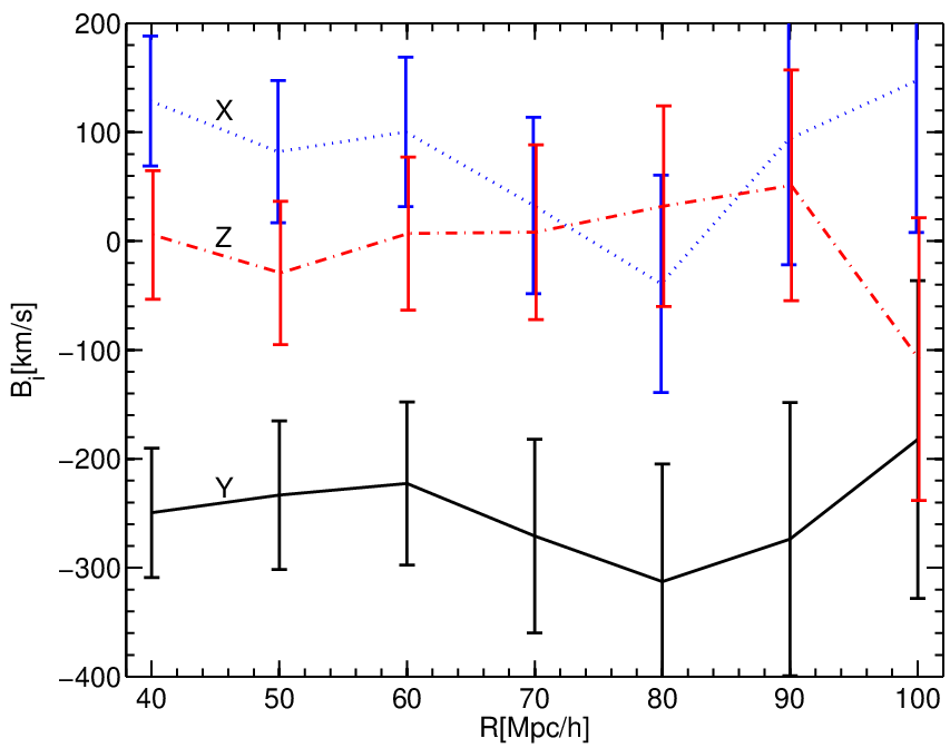
The description of the method presented in the previous Section assumes that the luminosities of galaxies in the sample are drawn from a single luminosity function. However, the method could easily be extended to account for the different luminosity functions of different galaxy types (e.g. red vs. blue, spirals vs. ellipticals) and environments (high density vs. low density regions). For this reason we have divided galaxies in two samples: spirals and ellipticals, and measured their luminosity functions separately. We find for early-type and , for late-type galaxies in agreement with the previous, independent estimates by [43]. We made no attempt to determine which is not relevant for our goal. These are the reference values for the luminosity function of the whole survey. To determine the bulk flow we consider a spherical subvolume of radius that contains 16460 galaxies brighter than , of which 10366 and 6094 are late and early types, respectively. We divided this sample into spherical shells each one thick. To estimate the three Cartesian components of the bulk flow, , in each shell, we have minimized the probability function with respect to , where the summation is over all galaxies in the shell. The expression for (20) is used for where different values of and are used for late and early type galaxies. The results are shown in Fig. 1. The points represent the Cartesian components of the bulk flow, indicated on the plot, estimated in correspondence of the mean radius of each shell. The errorbars were obtained from 200 mock samples mimicking the 2MRS subvolume. Each sample contains a number of points similar to that of the 2MRS galaxies. The points are randomly distributed within a sphere of and are assigned absolute magnitudes according to the overall reference luminosity function of all 2MRS galaxies. Mock galaxies were assigned random peculiar velocities sampled from a Gaussian distribution with zero mean and a scatter to mimic the combined effect of small scale velocity dispersion and errors in the measured redshift. No bulk flow was assigned to the mock samples. Our minimization procedure was then applied to the 200 mock samples to derive the intrinsic uncertainties in the estimate of the bulk flow. These uncertainties are plotted as errorbars.
Despite the large errors on the bulk from K=11.25 2MRS, the results are very encouraging. They provide a strong incentive for a more thorough study using the deeper K=12.2 2MRS which will triple number of galaxies within . The results can be compared with bulk flow of [29] (see their figure 5) obtained using the Tully-Fisher SFI++ data. A full comparison between the photometric and the SFI++ results is complicated and should take into account the complex covariance of errors in both measurements. The effort is redundant at this stage due to the large errors on the current 2MRS photometric bulk flow. Therefore, we only make a comparison between the two bulk flows at . At this intermediate radius the photometric bulk and the SFI++ (see top panel of figure 5 in [29]) are fully consistent. We note that refers to shells of thickness , while to the full sphere within . But this hardly matters since versus distance is nearly flat within the errors. The reason that is computed for shells rather than the whole spheres is that the bulk is heavily weighted by the lower redshifts galaxies due to the rapid decrease in the number of 2MRS galaxies at larger redshfits. Computing the photometric bulk in spherical shells allows a clearer inspection of the constraints we get at larger redshifts. In contrast, the SFI++ flow within a sphere of radius is, however, mainly dominated by galaxies nearer to .
The method outlined above is not the only one to estimate the bulk velocity of a spherical volume centered on the MW. We have implemented an alternative procedure based on the fact that a bulk flow, , introduces a dipole-like angular modulation in across a spherical shell centered on the observer. For , , where is the usual unit vector in the line-of-sight to the galaxy. The bulk flow, , can then be found by minimizing We have checked that this alternative strategy gives results that are noisier than but consistent with the luminosity-based method which uses the shape of the luminosity function, in addition to the measured magnitudes and redshifts.
IV Prospects for future surveys
In this section we assess the potential of our method applied to future datasets. The main goal of most of the next-generation large redshift survey is to constrain Dark Energy properties. For this reason, they are designed to optimize observations at , i.e the epoch at which Dark Energy started dominating the energy budget of the Universe. However, some of these projects will also provide redshifts, measured either spectroscopically or through multi-band photometry, for a large number of relatively local galaxies (i.e. ), where the bulk flow can be reliably estimated by our photometry-based method. Among the planned redshift surveys that meet these constraints are the ground-based LSST project [26] and the EUCLID satellite mission [25]. The two surveys enjoy the same large sky coverage ( deg2) and are expected to deliver photometric redshifts for a large (2-4 billion) number of galaxies in the redshift range . In addition, the EUCLID project is also expected to measure spectroscopic redshifts for about 70 million galaxies. Given the present uncertainties in the survey design we do not attempt here to provide an accurate forecast for the possibility of measuring our bulk flows from these surveys. Instead, we will allow for generous variations in the survey design parameters and provide an order of magnitude estimate for our capability to constraint the bulk flow at . For this purpose we will use the EUCLID survey as a baseline and allow for significant variations in the number of the objects in the survey which should include the case of the LSST survey.
To model the characteristic of both redshift surveys, the spectroscopic and the photometric ones, we need to specify the luminosity function of the galaxies, their redshift distribution and the errors on the photometry and the redshift.
For the luminosity function one we consider a Schechter form in the HAB-band with values of and derived from [6] assuming the H-K color correction proposed by [21]. The luminosity function evolves with redshift. Here we are interested in two epochs: and , for which we find and ,respectively. The spectroscopic catalog is expected to contain objects with apparent magnitude brighter tha H while the photometric catalog will sample galaxies as faint as H. We assume a photometric error which represents the expected error for faint objects and thus overestimate the uncertainties for brighter objects. We note that the expected number of objects in the EUCLID photo-z catalog ( gals. deg-2 with H) is remarkably similar to that in the LSST one ( gals. deg-2 with i). A similarity that also applies to the expected galaxy redshift distribution and that further justifies our choice of not considering the two surveys separately.
The galaxy redshift distribution for the EUCLID spectroscopic catalog has been modeled by [13]. In the current design, the survey will target galaxies above a limiting flux . The of these objects is listed in Table 2, column 3 of that paper. The numbers must be further divided by a factor to account for the efficiency in the determining the redshift from the line (Guzzo, private communication). This survey will measure the spectroscopic redshift of objects with with an expected accuracy . In the redshift bin centered at , the expected number of galaxies is . To simplify our calculation we adopt a more conservative and also explore the pessimistic case of measuring only redshifts.
The expected number of galaxies in the photo-z catalog can be derived by the observed galaxy the GOODS and UKIDDS-UDS fields (Zamorani, private communication). This catalog will include low-redshift objects and redshift will be measured with an accuracy (expected-goal). Here we adopt the first, more conservative estimate. At the number of objects in this catalog is 10 times larger than in the spectroscopic one, i.e. the same shell at considered above will have objects with measured photo-z. As before, we will also consider two pessimistic cases in which the number of measured redshifts is and . In the following we will be also interested in measuring the bulk flow in the nearby universe, at . At this distance EUCLID is expected to measure photo-z in a sphere of radius Mpc. We consider this as a reference number density at but also consider a pessimistic and an optimistic cases in which and , respectively.
To investigate whether our method can be applied successfully to these next-generation surveys we consider two possible estimates of the bulk flow: at and at . As a first example we consider a bulk flow in a sphere of radius Mpc at , similar in size to the one we have considered in the 2MRS sample. As a second case we consider a large bulk flow of a shell at with , reminiscent of the recent claimed detection by [22] and potentially conflicting with the standard cosmological framework. These two bulk flows introduce the same systematic shift in the apparent magnitude of the objects: . Our task is to assess if the next generation surveys described above will be able to detect such shift. To summarize, we will explore the following scenarios:
- •
The case of a spherical region of radius Mpc moving at at , containing objects with measured photo-z. In addition to this reference case we also consider an optimistic and pessimistic scenarios in which the number of measured photometric redshifts is and , respectively. The results relative to this scenario are listed in the first 12 rows of Table 1.
- •
The case of a shell at centered on the MW, with and moving , sampled by objects with measured photo-z (reference case). We also consider the pessimistic cases of and objects. The results relative to this scenario are listed in rows 13-24 of Table 1.
- •
The case of the same shell at moving at the same speed but sampled by with redshift measured spectroscopically. We also consider a more pessimistic case of objects. The results are listed in rows 25-26 of Table 1.
The general strategy to assess our ability in measuring the bulk flow is straightforward. First, we consider a very large set of objects representing the whole survey to which we assign absolute magnitudes according to the reference luminosity function and determine the and by minimizing . Then, for each of the three scenarios itemized above, we repeat the exercise considering 70 subsamples, i.e. we determine a set of (,) values by minimizing . Objects in the subsamples are assigned a magnitude error by adding a Gaussian scatter of zero mean and width and no bulk flow. The condition for a significant bulk flow detection is that the rms scatter in the value of measured from the 70 mock samples is larger than the expected magnitude shift
The results of this test are summarized in Table 1. They refer to the three scenarios outlined above. To assess the impact of photometric errors we have explored the case of (no photometric errors) and that of fixing at its mean value as derived from the mean of subsamples. In this Table, is the difference between the mean of the recovered from the 70 subsamples and the true value and its scatter . The quantities and are defined similarly but for .
For , we get very small and . This means that one can treat the corresponding values as those that would be obtained from the full survey (which is expected to contain a significantly large number of galaxies than ). Since the presence of a bulk flow is not expected to affect but only , this result suggests that one can safely fix to the value measured from the whole survey, i.e. that the case which is directly relevant for our method is the one tagged ’fixed in Table 1. We also show the case of free for the sake of completeness. The results also show that when the values of and vanish. This is a known effect and reflects the fact that random photometric errors preferentially scatter galaxies to the brighter end of the luminosity function. However, the bias would affect the estimate of the true luminosity function from the whole survey and hence it is irrelevant to our method which only uses the values of and measured from the full survey in order to get the bulk flow by minimization of .
The results show that the bulk flows that we are considering here and which would introduce a systematic magnitude shift would be detected at high significance in all three reference cases considered (boldface quantities in Table 1). In particular, we see that the bulk flow at would be detected at significance by measuring the photometric redshift of objects in a a sphere of Mpc. At , photometric redshifts would allow us to detect a bulk flow of at , decreasing to , respectively, for and photometric redshifts. The statistical significance of the bulk flow detection can be further increased by reducing redshift errors, i.e. by using spectroscopic rather than photometric redshifts. The result is seen by comparing the two cases of a spectroscopic and a photo-z with the same value of and , (e.g. row 25 vs. row 20 in Table 1). The value of is reduced by a factor of . The reason of this improvement is that galaxies in the spectroscopic catalog sample the brighter end of the luminosity function which is sensitive to the value of . The result is that, for the same value of , the galaxies in the spectroscopic sample are able to constrain considerably better than galaxies in the photometric catalog. The same reasoning explains why in row 16, which refers to a sample of distant, bright galaxies at is smaller than the value in row 4 which refers to a sample of nearer and fainter galaxies.
| row # | |||||
|---|---|---|---|---|---|
| 1 | 0.13 | ||||
| 2 | 0.13 | fixed | |||
| 3 | 0.13 | ||||
| 4 | 0.13 | fixed | |||
| 5 | 0.13 | ||||
| 6 | 0.13 | fixed | |||
| 7 | 0.13 | ||||
| 8 | 0.13 | fixed | |||
| 9 | 0.13 | ||||
| 10 | 0.13 | fixed | |||
| 11 | 0.13 | ||||
| 12 | 0.13 | fixed | |||
| 13 | 0.5 | ||||
| 14 | 0.5 | fixed | |||
| 15 | 0.5 | ||||
| 16 | 0.5 | fixed | |||
| 17 | 0.5 | ||||
| 18 | 0.5 | fixed | |||
| 19 | 0.5 | ||||
| 20 | 0.5 | fixed | |||
| 21 | 0.5 | ||||
| 22 | 0.5 | fixed | |||
| 23 | 0.5 | ||||
| 24 | 0.5 | fixed | |||
| 25 | 0.5 | fixed | |||
| 26 | 0.5 | fixed |
V Discussion
Over the years cosmological bulk flows has been estimated from the measured peculiar velocities of a large variety of objects ranging from galaxies [14, 15, 12, 7, 9, 37] clusters of galaxies [24, 5, 18] and SNIa [36]. Conflicting results triggered by the use of error-prone distance indicators have fueled a long lasting controversy on the amplitude and convergence of the bulk flow that is still on. For example, using the SFI++ galaxy catalog [42], claimed the detection of a bulk flow of km s-1 within Mpc, inconsistent with expectation from the CDM model. This result has been challenged by the re-analysis of the same data by [30] who found a bulk flow amplitude consistent with CDM expectations. Several bulk flow estimates have been recently performed from the dipole-like anisotropy induced by the kinetic Sunyaev-Zel’dovich decrement in the WMAP temperature map, measured at the position of X-ray galaxy clusters. When interpreted as a coherent motion, this signal would indicate a gigantic bulk flow of km s-1 within Mpc, clearly inconsistent with the standard picture of gravitational instability. However, a more recent and independent analysis of WMAP data [32] did not confirm this result. Finally, systematic anisotropies in the observed clustering of objects induced by peculiar velocities, the so called redshift space distortions, are a popular and reliable way to estimate the growth rate of density fluctuations and to constrain the amplitude of large-scale coherent motions [34, 16, 3]. However, their interpretation in terms of bulk velocity is not straightforward.
Here we have presented and implemented a method to estimate cosmological bulk flows that only depends on photometry and redshift measurements and not on distance indicators. The main requirements for a successful application of this statistical method is dense sampling over large regions of the universe. A large number of object is mandatory since, for a given bulk flow amplitude, errors are dominated by Poisson noise, as clearly indicated by the fact that the error on , , listed in Table 1 scales as . We find that the accuracy in the measurement of galaxy magnitude and redshifts are less crucial in the bulk flow estimate. This fact indicates that photometric-redshift catalogs are better suited for this analysis than the spectroscopic ones which typically include significantly less galaxies. Of course, this assumes that systematic errors and the fraction of outliers (which can be significant at [26]) in the photo-z measurement can be conveniently reduced. Dedicated analysis that accurately mimic the expected performance of the surveys will be required to address this issue.
Large volumes and dense sampling are requirements that will be met by next-generation redshift surveys like EUCLID and LSST. Therefore, we have carried out a feasibility study for such surveys. Taking into account that the sensitivity of our method decreases with the redshift we have only considered galaxies with . We focused on two different measurements: a bulk flow of at on scales and a much larger bulk flow of at over a shell centered on the MW. Both flows would introduce the same shift in the measured magnitude of the galaxies. The results, summarized in Table 1 are very encouraging. They suggests, for example, that one could obtain independent estimates of cosmological bulk flows (with typical amplitude of ) over the 2MRS-sized samples within It is worth stressing that photo-z are accurate enough for our purposes. A comparison between rows 8 and 25 in the Table shows that galaxies (with photo-z) the error in determining is actually smaller at than . This implies that a bulk flow of (which amounts to at and at ) is constrained at the level at both redshifts.
As a preliminary application of the method, we have resorted to the 2MRS all sky survey which is limited to . The results are consistent with the bulk flow derived by [29] using the SFI++ Tully-Fisher catalog of distance indicators. The 2MRS photometric bulk flow derived here is noisy due to the relatively small number of galaxies. Better results will be obtained using the deeper 2MRS. This already planned extension of the original survey will increase the number of observed redshifts by a factor of 3 within a distance of . Since Poisson noise dominates the error budget, we expect a factor of reduction in the size of the errorbars.
There are strong indications that the luminosity function, , depends on the large scale environment of galaxies [2, 19, 8, 33, 28, e.g.]. These studies explore the dependence on the density of galaxies on scales of a few Mpcs. As outlined above, we are interested in significantly larger scales of . When averaged over these scales, the rms density fluctuations is less than 0.07 (for standard CDM model with ). So far no study has addressed environmental dependences of galaxy luminosities over such large scales. If the overdensity of the large scale environment is the main relevant parameter, then an extrapolation of the observed dependence on a few Mpc scales to 100 yields an exceedingly small effect. Moreover, in next generation surveys we could easily account for such effects thanks to our ability to measure the bulk flow over independent volumes that could be classified according to their average density. To illustrate the robustness of our 2MRS result over environmental effects, we note that a 300 bulk flow at gives a magnitude difference of between the apex and the anti-apex of the bulk motion. In CDM, the rms density in spheres of is 0.13. Assuming again that the overdensity of the environment is the only relevant parameter, we find that should dominate the environmental dependence extrapolated from smaller scales. A further evidence that environmental effects did not affect our bulk flow estimates from 2MRS is that the method here gives results that are consistent with those [29] who derive the bulk flow based on the Tully-Fisher distant indicators, rather than photometry.
VI Acknowledgments
This work was supported by THE ISRAEL SCIENCE FOUNDATION (grant No.203/09), the German-Israeli Foundation for Research and Development, the Asher Space Research Institute and by the WINNIPEG RESEARCH FUND. MD acknowledges the support provided by the NSF grant AST-0807630. EB acknowledges the support provided by the Agenzia Spaziale Italiana (ASI, contract N.I/058/08/0) EB thanks the Physics Department and the Asher Space Science Institute-Technion for the kind hospitality.
References
- [1] Arfken, G. B., & Weber, H. J. 2005, Mathematical methods for physicists 6th ed. (Elsevier)
- [2] Balogh, M. L., Christlein, D., Zabludoff, A. I., & Zaritsky, D. 2001, ApJ, 557, 117
- [3] Blake, C., Brough, S., Colless, M., Couch, W., Croom, S., Davis, T., Drinkwater, M. J., Forster, K., Glazebrook, K., Jelliffe, B., Jurek, R. J., Li, I., Madore, B., Martin, C., Pimbblet, K., Poole, G. B., Pracy, M., Sharp, R., Wisnioski, E., Woods, D., & Wyder, T. 2010, MNRAS, 406, 803
- [4] Blakeslee, J. P., Davis, M., Tonry, J. L., Dressler, A., & Ajhar, E. A. 1999, ApJL, 527, L73
- [5] Branchini, E., Plionis, M., & Sciama, D. W. 1996, ApJL, 461, L17+
- [6] Cirasuolo, M., McLure, R. J., Dunlop, J. S., Almaini, O., Foucaud, S., & Simpson, C. 2010, MNRAS, 401, 1166
- [7] Courteau, S., Willick, J. A., Strauss, M. A., Schlegel, D., & Postman, M. 2000, ApJ, 544, 636
- [8] Croton, D. J., Farrar, G. R., Norberg, P., Colless, M., Peacock, J. A., Baldry, I. K., Baugh, C. M., Bland-Hawthorn, J., Bridges, T., Cannon, R., Cole, S., Collins, C., Couch, W., Dalton, G., De Propris, R., Driver, S. P., Efstathiou, G., Ellis, R. S., Frenk, C. S., Glazebrook, K., Jackson, C., Lahav, O., Lewis, I., Lumsden, S., Maddox, S., Madgwick, D., Peterson, B. A., Sutherland, W., & Taylor, K. 2005, MNRAS, 356, 1155
- [9] da Costa, L. N., Bernardi, M., Alonso, M. V., Wegner, G., Willmer, C. N. A., Pellegrini, P. S., Maia, M. A. G., & Zaroubi, S. 2000, ApJL, 537, L81
- [10] Dai, D., Kinney, W. H., & Stojkovic, D. 2011, ArXiv:1102.0800
- [11] Davis, M., Nusser, A., Masters, K. L., Springob, C., Huchra, J. P., & Lemson, G. 2011, MNRAS, 413, 2906
- [12] Dekel, A., Eldar, A., Kolatt, T., Yahil, A., Willick, J. A., Faber, S. M., Courteau, S., & Burstein, D. 1999, ApJ, 522, 1
- [13] Geach, J. E., Cimatti, A., Percival, W., Wang, Y., Guzzo, L., Zamorani, G., Rosati, P., Pozzetti, L., Orsi, A., Baugh, C. M., Lacey, C. G., Garilli, B., Franzetti, P., Walsh, J. R., & Kümmel, M. 2010, MNRAS, 402, 1330
- [14] Giovanelli, R., Haynes, M. P., Freudling, W., da Costa, L. N., Salzer, J. J., & Wegner, G. 1998a, ApJL, 505, L91
- [15] Giovanelli, R., Haynes, M. P., Salzer, J. J., Wegner, G., da Costa, L. N., & Freudling, W. 1998b, AJ, 116, 2632
- [16] Guzzo, L., Pierleoni, M., Meneux, B., Branchini, E., Le Fèvre, O., Marinoni, C., Garilli, B., Blaizot, J., De Lucia, G., Pollo, A., McCracken, H. J., Bottini, D., Le Brun, V., Maccagni, D., Picat, J. P., Scaramella, R., Scodeggio, M., Tresse, L., Vettolani, G., Zanichelli, A., Adami, C., Arnouts, S., Bardelli, S., Bolzonella, M., Bongiorno, A., Cappi, A., Charlot, S., Ciliegi, P., Contini, T., Cucciati, O., de la Torre, S., Dolag, K., Foucaud, S., Franzetti, P., Gavignaud, I., Ilbert, O., Iovino, A., Lamareille, F., Marano, B., Mazure, A., Memeo, P., Merighi, R., Moscardini, L., Paltani, S., Pellò, R., Perez-Montero, E., Pozzetti, L., Radovich, M., Vergani, D., Zamorani, G., & Zucca, E. 2008, Nature, 451, 541
- [17] Huchra, J., Jarrett, T., Skrutskie, M., Cutri, R., Schneider, S., Macri, L., Steining, R., Mader, J., Martimbeau, N., & George, T. 2005b, in Astronomical Society of the Pacific Conference Series, Vol. 329, Nearby Large-Scale Structures and the Zone of Avoidance, ed. A. P. Fairall & P. A. Woudt, 135–+
- [18] Hudson, M. J., Smith, R. J., Lucey, J. R., & Branchini, E. 2004, MNRAS, 352, 61
- [19] Hütsi, G., Einasto, J., Tucker, D. L., Saar, E., Einasto, M., Müller, V., Heinämäki, P., & Allam, S. S. 2002, ArXiv:astro-ph/0212327
- [20] Jarosik, N., Bennett, C. L., Dunkley, J., Gold, B., Greason, M. R., Halpern, M., Hill, R. S., Hinshaw, G., Kogut, A., & et. al. 2010, ArXiv e-prints
- [21] Jimenez, R., & Kashlinsky, A. 1999, ApJ, 511, 16
- [22] Kashlinsky, A., Atrio-Barandela, F., Ebeling, H., Edge, A., & Kocevski, D. 2010, ApJL, 712, L81
- [23] Larson, D., Dunkley, J., Hinshaw, G., Komatsu, E., Nolta, M. R., Bennett, C. L., Gold, B., Halpern, M., & Hill, e. a. 2010, ArXiv e-prints
- [24] Lauer, T. R., & Postman, M. 1994, ApJ, 425, 418
- [25] Laureijs, R. 2009, ArXiv:0912.0914
- [26] LSST Science Collaborations, Abell, P. A., Allison, J., Anderson, S. F., Andrew, J. R., Angel, J. R. P., Armus, L., Arnett, D., Asztalos, S. J., Axelrod, T. S., & et al. 2009, ArXiv:0912.0201
- [27] Masters, K. L., Springob, C. M., Haynes, M. P., & Giovanelli, R. 2006, ApJ, 653, 861
- [28] Mo, H. J., Yang, X., van den Bosch, F. C., & Jing, Y. P. 2004, MNRAS, 349, 205
- [29] Nusser, A., & Davis, M. 2011a, ArXiv:1101.1650
- [30] —. 2011b, ArXiv e-prints
- [31] Nusser, A., Dekel, A., Bertschinger, E., & Blumenthal, G. R. 1991, ApJ, 379, 6
- [32] Osborne, S. J., Mak, D. S. Y., Church, S. E., & Pierpaoli, E. 2010, ArXiv e-prints
- [33] Park, C., Choi, Y., Vogeley, M. S., Gott, III, J. R., & Blanton, M. R. 2007, ApJ, 658, 898
- [34] Peacock, J. A., Cole, S., Norberg, P., Baugh, C. M., Bland-Hawthorn, J., Bridges, T., Cannon, R. D., Colless, M., Collins, C., Couch, W., Dalton, G., Deeley, K., De Propris, R., Driver, S. P., Efstathiou, G., Ellis, R. S., Frenk, C. S., Glazebrook, K., Jackson, C., Lahav, O., Lewis, I., Lumsden, S., Maddox, S., Percival, W. J., Peterson, B. A., Price, I., Sutherland, W., & Taylor, K. 2001, Nature, 410, 169
- [35] Riess, A. G., Davis, M., Baker, J., & Kirshner, R. P. 1997, ApJL, 488, L1+
- [36] Riess, A. G., Press, W. H., & Kirshner, R. P. 1995, ApJL, 445, L91
- [37] Sarkar, D., Feldman, H. A., & Watkins, R. 2007, MNRAS, 375, 691
- [38] Schechter, P. L. 1980, Astronomical Journal, 85, 801
- [39] Springob, C. M., Masters, K. L., Haynes, M. P., Giovanelli, R., & Marinoni, C. 2007, ApJ. S, 172, 599
- [40] Tammann, G. A., Yahil, A., & Sandage, A. 1979, ApJ, 234, 775
- [41] Tully, R. B., & Fisher, J. R. 1977, A&A, 54, 661
- [42] Watkins, R., Feldman, H. A., & Hudson, M. J. 2009, MNRAS, 392, 743
- [43] Westover, M. 2007, PhD thesis, Harvard University