Phase structure of a three-diensional Yukawa model
Abstract
We use the method of the exact renormalization group to study the renormalization group flows of an O(N) invariant Yukawa model in three dimensional Euclidean space consisting of one real scalar and N real spinor fields. We obtain a phase structure similar to that of the N-vector model with cubic anisotropy, possessing a region of parameters exhibiting a first order transition. The particular case with one real fermion (N=1) belongs to the same universality class as the Wess-Zumino model with one supersymmetry. For the critical exponents of the Wilson-Fisher type fixed points, our 1-loop approximations are generally consistent with the results of previous studies.
1 Introduction
The purpose of this paper is to study a model of a real scalar field interacting with an arbitrary number of real spinor fields in three dimensional space-time. As is well known, the properties of a spinor such as the number of independent components depend highly on the dimensionality of space-time. [1] In three dimensional space-time, spinors transform under , and the real and imaginary parts do not mix. Under dimensional reduction, a Majorana spinor (or equivalently a Weyl spinor and its complex conjugate) in four dimensional space-time gives a complex spinor in three dimensions, which is a pair of real spinors. Hence, a single real spinor is intrinsically an object in three dimensional space-time. Our model with an odd number of spinors cannot be obtained from a four dimensional model by dimensional reduction. Therefore, we need a formalism that caters specifically to the three dimensional space-time.
We study our model using the framework of the exact renormalization group (ERG) upon which reviews from various viewpoints are available. [2, 3, 4, 5, 6, 7, 8, 9, 10, 11] ERG is known for its successes in non-perturbative applications to many different areas of physics such as critical phenomena, gauge theories, lattice models, non-relativistic few-body problems, strongly correlated electrons, and quantum gravity. [12]
In this paper we are particularly interested in obtaining the phase structure of our model. To obtain the phase structure it is sufficient to derive the RG flows. To simplify this task, we restrict our model so that it is accessible from the Gaussian fixed point. With the symmetry among real fermions, this choice leaves only three parameters to consider. Since we are mainly interested in understanding the general features of the model, we do not attempt to take advantage of the full potential of ERG. We solve the ERG differential equation for the Wilson action perturbatively at 1-loop level to derive the RG flows of the parameters.
The primary finding of this paper is the phase structure similar to that of the N-vector model with cubic anisotropy. [13] We find two non-trivial fixed points (besides the fixed point of the theory). One is the Wilson-Fisher type with only one relevant parameter. [14] For , this is the same as the fixed point of the supersymmetric Wess-Zumino model. For even, this is the fixed point of the Gross-Neveu model with complex fermions. [15] The other fixed point has two relevant directions, and its existence implies a region of the parameter space that exhibits a first order transition.
Our work has been partially motivated by a recent work on the supersymmetric Wess-Zumino model in three dimensions [16], where a non-trivial Wilson-Fisher type fixed point has been discovered. Our model includes the supersymmetric model as a subset, and we expect to obtain the same fixed point without imposing supersymmetry. If is even, the model can be rewritten for complex fermions, and this class of models has been studied with ERG in Ref. \citenRosa:2000ju, where the flow equation is solved numerically with the initial condition corresponding to the Gross-Neveu model.
The paper is organized as follows. In §2 we introduce our model and discuss its symmetry. In §3 we define the Wilson action and its parameters. In §4 we derive RG flows and find fixed points. In §5 we discuss the nature of the phase transition shown by the model. In §6 (for ) and §7 (for even) we compare our results with those of previous studies. Finally, in §8 we conclude the paper with remarks. The extensive appendices provide technical details that make the paper self-contained.
Throughout the paper we work in three dimensional Euclidean space, and we use the following notation for momentum integrals:
| (1) |
2 Yukawa model
We consider a model whose classical lagrangian is given by
| (2) |
where is a real scalar, and are real spinors. (See Appendix A for the corresponding lagrangian in Minkowski space.) We denote
| (3) |
We adopt the Einstein convention for summation over the repeated index .
The lagrangian is invariant under the following transformation
| (4) |
This invariance forbids the mass term . Depending on how this discrete symmetry is realized, we expect two phases:
- 1.
exact — The expectation value of the scalar vanishes , and the fermions stay massless.
- 2.
spontaneously broken — , and the fermions become massive.
In both phases we expect the symmetry among real fermions are unbroken.
For , we expect that the model belongs to the same universality class as the Wess-Zumino model whose classical lagrangian is given by
| (5) |
where
| (6) |
The Wess-Zumino model is a subset of the Yukawa model, satisfying the relation
| (7) |
Hence, the critical exponents of the Wess-Zumino model must be the same as those of the Yukawa model.
For , the Yukawa model also belongs to the same universality class as the three dimensional Gross-Neveu model given by
| (8) |
We expect again that the critical exponents are the same as those of the Yukawa model. (See Fig. 1.) For even, the model contains complex fermions; defining complex fermions
| (9) |
for , we can write
| (10) |
(See appendix A for complex fermions.)

3 Wilson action
We construct a Wilson action that depends on a UV cutoff in such a way that its physics is independent.[14] The Wilson action is split into two parts:
| (11) |
The free part is given by
| (12) |
The cutoff function is positive, at , and decays fast enough for . To make the physics independent of , we impose that the interaction part satisfy the ERG differential equation [18]
| (13) | |||
where
| (14) |
To determine uniquely, we must introduce two additional conditions [19, 20]:
- 1.
UV renormalizability — We impose that the theory becomes the free massless theory at short distances. We demand the following asymptotic conditions:
(15) where the terms with higher powers of fields vanish, and all the coefficients are constant except for which has a part linear in and another linear in .
- 2.
Introduction of couplings , — We expand the Wilson action in powers of fields to obtain
(16) Choose a finite renormalization scale . We then impose
(17) The first four are normalization conditions, and the last two introduce coupling constants & . Note that the squared mass parameter is introduced through .
The conditions (13-17) determine uniquely as a functional of & ; depends on the parameters and the mass scales . also depends on a particular choice of the cutoff function , but it can be shown formally that the dependence can be absorbed by the normalization of parameters and fields. (For example, see Appendix B.2 of Ref. \citenIgarashi:2009tj.)
The beta functions and anomalous dimensions are obtained as the dependence of the Wilson action [19, 20]:
| (18) |
The operators are defined by
| (19) | |||||
| (20) | |||||
| (21) |
These generate infinitesimal changes of the parameters , respectively. Denoting the independent correlation functions by brackets, we obtain
| (22) |
where the dots stand for a string of elementary fields and . The operators and are the equation-of-motion operators defined by
| (23) | |||||
| (24) |
where
| (25) | |||||
| (26) |
They count the number of fields in the correlation functions:
| (27) |
The meaning of (18) is clear. Its correlation with a product of elementary fields gives the RG equation:
| (28) |
where are the number of ’s and ’s in the correlator.
In order to compute the beta functions at 1-loop, we need to compute at 1-loop, in particular the coefficients . The results are given in Appendix B. Taking the derivatives, we obtain the following results:
| (29) | |||||
| (30) | |||||
| (31) | |||||
| (32) | |||||
| (33) |
where the integrals ’s are defined in terms of the cutoff function and its derivative in Appendix E.
4 RG equations and fixed points
We have obtained 1-loop beta functions and anomalous dimensions. To obtain RG flows that describe the phase structure of the Yukawa model, we need to rescale both space and fields so that the renormalization scale is fixed under the RG flows. Due to this resclaing, the beta functions acquire contribution from the engineering dimensions of the parameters. Calling as , as , and as , the flow equations for these dimensionless parameters become
| (34) |
These equations are valid in a neighborhood of the origin , called the Gaussian fixed point. As has been explained in §1, we restrict ourselves only to the region of parameters accessible from the Gaussian fixed point. In other words, we only follow the flows that originate from the origin. All the non-trivial fixed points we will discuss in this section are accessible from the Gaussian fixed point.
At 1-loop, using the results of the previous section, we obtain
| (35) |
where the integrals ’s are defined in terms of the cutoff function in Appendix E, and by
| (36) |
and by
| (37) |
With the convention , we obtain
| (38) |
Similarly, the anomalous dimensions are given by
| (39) |
which are independent of .
The RG flows are given schematically in Fig. 2.

For any , the flows have four fixed points.
- 1.
Gaussian — This exists by construction; in this paper we only study the RG flows out of this fixed point. At the Gaussian fixed point, all parameters vanish:
(40) - 2.
Ising — With , the fermions decouple, and we get a theory. Its fixed point corresponds to the critical Ising model.
(41) The small deviation has the scale dimension
(42) Similarly, has the scale dimension . and are the two relevant parameters at this fixed point.
- 3.
Wilson-Fisher — This is the most stable fixed point given by
(43) where is given explicitly by (38). The scale dimension of is given by
(44) is the only relevant parameter. is irrelevant with the scale dimension
(45) - 4.
Bicritical — This has two relevant parameters, and we call this a bicritical fixed point.
(46) where , the scale dimension of , is given by
(47) Unlike the Wilson-Fisher fixed point, is relevant with the scale dimension
(48)
| parameter | Gauss | Ising | Wilson-Fisher | Bicritical |
|---|---|---|---|---|
The critical exponents are universal, and accordingly they do not depend on what cutoff function we use to formulate the ERG differential equations.[21] (See also Appendix B.2 of Ref. \citenIgarashi:2009tj.) Approximate solutions of the ERG differential equations, whether they are perturbative or non-perturbative, lose universality, and the critical exponents become dependent on the choice of a cutoff function. The cutoff dependence is an inevitable artifact of the introduction of an approximation.
To compute the critical exponents numerically, we have used a particular class of (See Fig. 10 in Appendix E):
| (49) |
The advantage of this cutoff function is that the necessary 1-loop integrals, listed in Appendix E, can be performed analytically. The cutoff function interpolates two popular choices, one at (Litim’s cutoff [22]) and another at (sharp cutoff [23]). The dependence of the critical exponents on the parameter indicates the accurracy of the numerical values obtained.
Let us plot the -dependence of the critical exponents for . (Fig. 3) We find that the exponents do not have much -dependence for . takes a maximum value at , a maximum at , and a maximum at . Since , takes a minimum at .

We take these extremum values as our numerical estimates for the exponents. [24] Note that the following relations are satisfied:
| (50) |
Hence, at the bicritical fixed point, is more relevant than . We next plot the -dependence of the anomalous dimensions (Fig. 4):
| (51) |
At 1-loop, the Wilson-Fisher and bicritical fixed points share the same anomalous dimensions. Again, the dependence on is mild in the region . The extremum values at are
| (52) |

5 Phase transitions
Given & , we examine the dependence of the model on the squared mass parameter in this section.
Suppose is in Region 1, surrounded by four RG flows G-I, I-WF, B-WF, and G-B in Fig. 2. Then the two-dimensional flow is always attracted to the Wilson-Fisher fixed point. Let be the value of such that the RG flow starting from flows to the Wilson-Fisher fixed point as :
| (53) |
Since , the deviation is relevant, and grows along the RG flow. Hence, the model exhibits a continuous phase transition at . We expect that the is exact for and broken for .
Let us now suppose is in Region 2, to the left of the RG flow G-B in Fig. 2. The two-dimensional flow has no fixed point to reach, and this implies the existence of a transition point that exhibits a first order phase transition. As for Region 1, we expect that the is exact for and broken for . In Appendix C we compute and by solving the 1-loop RG equations analytically. (For the first order transition, only the infinitesimal region below G-B is considered.)
The phase structure of the Yukawa model discussed above is similar to that of the N-vector model with cubic anisotropy in dimensions. [13] (See also §5.8.5 of Ref. \citenChaikin:1995, for example.) The classical lagrangian of the model is given by
| (54) |
where . The phase structure depends on , but it is similar to the phase structure of the Yukawa model found here with the presence of a region of first order transitions. (Fig. 5)

6 Comparison of the case with the Wess-Zumino model
The case is particularly interesting since the model belongs to the same universality class as the supersymmetric Wess-Zumino model. The Wess-Zumino model has recently been studied with ERG, [16] and we would like to make sure that our results are compatible.
The Wilson-Fisher fixed point is characterized by three critical exponents: , , and . Supersymmetry implies
| (55) |
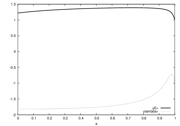
As Fig. 4 shows, this relation is satisfied at the extremum , and reasonably satisfied for . An interesting relation
| (56) |
found in Ref. \citenSynatschke:2010ub is also reasonably satisfied for . (Fig. 4) Considering the crudeness of our 1-loop approximations, the agreement is satisfactory.
| Yukawa | |||||
|---|---|---|---|---|---|
| Wess-Zumino [16] |
In Appendix D we apply our perturbative ERG formalism directly to the WZ model and compute the critical exponents. The agreement with Ref. \citenSynatschke:2010ub improves slightly.
7 Comparison with the Gross-Neveu model
Let us consider the large limit of the RG equations of sect. 4, which gives
| (57) |
The Gross-Neveu model with complex fermions has been studied with ERG in \citenRosa:2000ju, where the RG flow of the Yukawa model was run numerically with the initial condition corresponding to the Gross-Neveu model. In TABLE 3 the results of Ref. \citenRosa:2000ju are compared with ours for , evaluated at a peak near , and , evaluated at . (Fig. 6)


| ours | ||||||||
|---|---|---|---|---|---|---|---|---|
| Ref. \citenRosa:2000ju | ||||||||
In Ref. \citenHands:1991py, the critical exponents have been calculated to order as follows:
| (58) |
(We have replaced , the number of complex fermions, in Ref. \citenHands:1991py by , where is the number of real fermions.) Our results reproduce the correct large N limit, but not the corrections. The most serious failure of our 1-loop approximation is the wrong sign for the correction to ; in comparison the correct sign has been obtained in \citenRosa:2000ju.
We note that a first order transition was found for in Ref. \citenRosa:2000ju. This can be explained if we assume that the transition point of this model belongs to Region 1 of the parameter space. (Fig. 7)


8 Concluding remarks
In this paper we have applied the ERG formalism perturbatively to the Yukawa model in three dimensions to obtain the RG flows. We have found a phase structure similar to that of the N-vector model with cubic anisotropy. Accordingly, the spontaneous breaking of the symmetry of the Yukawa model can take place either at a continuous or at a first order transition point. The existence of a domain of parameters for the first order transition should be verified further, perhaps, by studying the effective potential with ERG.
The Yukawa model with one real spinor includes the Wess-Zumino model as a subset, and the fixed point of the latter is inevitably that of the former. At the Wilson-Fisher type fixed point of the Yukawa model, the only relevant parameter preserves supersymmetry; hence, the long distance behavior of an almost critical Yukawa model is the same as a massive Wess-Zumino model with its supersymmetry either exact or broken spontaneously. Emergence of supersymmetry at a critical point of a non-supersymmetric theory has also been found for the Yukawa model with complex scalars and spinors. [27]
The way we apply ERG perturbatively, we can only study the RG flows of UV renormalizable theories. This constraint still leaves a wide class of models as an object of study, and we advocate further perturbative applications of ERG for its simplicity and good cost-performance ratio.
Acknowledgements
I thank the organizers and participants of the ERG2010 conference held in Corfu, Greece for a stimulating atmosphere where partial results of this paper were presented. I also thank Yannick Meurice for critical comments and for Ref. \citenLee:2010fy. This work was partially supported by JSPS Grant-In-Aid #22540282.
Appendix A Spinors in
For the reader’s convenience, we summarize the salient features of spinors in three dimensional Minkowski and Euclidean spaces.
A.1 Minkowski space
We can choose the gamma matrices pure imaginary:
| (59) |
Under a Lorentz transformation, a two-component spinor transforms as
| (60) |
where is a 2-by-2 real matrix with determinant . Since is real, we can assume to be real. We define
| (61) |
which transforms as
| (62) |
since
| (63) |
The lagrangian of the Yukawa model is given by
| (64) |
This is invariant under the parity transformation defined by
| (65) |
The mass term is forbidden by this invariance.
A Dirac spinor is a linear combination of two real spinors:
| (66) |
We find
| (67) |
We obtain
| (68) |
A Dirac spinor can be obtained by the dimensional reduction of a Weyl (or Majorana) spinor in -dim Minkowski space.
A.2 Euclidean space
We can choose
| (69) |
corresponding to the spin representation, familiar from non-relativistic quantum mechanics. Under a space rotation, a two-component spinor transforms as
| (70) |
where . transforms as
| (71) |
Hence, the lagrangian
| (72) |
is invariant under .
We call a real fermion, and call a linear combination of two real fermions
| (73) |
a complex fermion. Denoting , we can write the lagrangian for as
| (74) |
and are two independent 2-component Grassmann fields.
Appendix B Wilson action at 1-loop
Defining
| (75) |
the 1-loop vertices are calculated as follows:
- 1.
scalar 2-point
(76) where the constant is given by
(77) - 2.
fermion 2-point
(78) where the constant is given by
(79) - 3.
Yukawa coupling
(80) - 4.
scalar 4-point
(81)
The asymptotic behaviors as are given by
| (82) | |||||
| (83) | |||||
| (84) | |||||
| (85) | |||||
Appendix C Analytic calculations of and
The 1-loop RG equations can be solved analytically. Hence, given arbitrary in Region 1, we can compute the critical value . Similarly, given in Region 2 near the line GB, we can compute the transition value . In this appendix, we first solve the flow equations, and then calculate and .
C.1 Solving the flow equations
The solution for is given by
| (88) |
We choose so that
| (89) |
Defining
| (90) |
we obtain
| (91) |
where is a constant determined by the initial condition, and
| (92) |

In Fig. 8, the three regions are defined by the behavior of :
| (93) |
is positive in , but negative in and . In , the region of a first order transition, we find (hence ) at a finite .
The flow equation for the squared mass is given by
| (94) |
where
| (95) |
This is solved as
| (96) |
C.2 Critical squared mass
In region , the critical value of is obtained as a function of and by the condition
| (97) |
This implies that the left-hand side of (96) vanishes in the limit . Hence, we obtain
| (98) |
Using the analytic solution for and , this can be rewritten as
| (99) |
where is the same as before except it is regarded now as a function of , and it is explicitly given by
| (100) |
C.3 First order transition point
We consider a region directly below the trajectory GB, which is a line given by
| (101) |
For and a positive infinitesimal ,
| (102) |
gives a point in just below the trajectory GB. The squared mass at the first order transition is obtained as
| (103) |
where
| (104) | |||||
and the derivative is given by
| (105) |
Appendix D ERG for the Wess-Zumino model in
To study the three dimensional Wess-Zumino model, it is the most convenient if we preserve supersymmetry manifestly by linearizing it with the help of a real auxiliary field . The corresponding classical lagrangian is
| (106) |
Integrating over , we reproduce the classical action given by (5) in sect. 2. The imaginary is necessary for the Euclidean space. The classical lagrangian is invariant under the following supersymmetry transformation:
| (107) |
where is an arbitrary constant spinor. Besides supersymmetry, the theory is invariant under the transformation:
| (108) |
We construct a Wilson action that is invariant under the linearized supersymmetry and transformation. (The invariance forbids the supersymmetric mass term .)
The Wilson action is split into the free and interaction parts:
| (109) |
where satisfies the ERG differential equation
| (110) | |||||
For UV renormalizability, we impose the following asymptotic behavior:
| (111) | |||||
where and are constants, and is linear in . (Note that in the common language the coefficient of is linearly divergent; supersymmetry is consistent with this divergence.) The parameters are introduced through the expansion:
| (112) | |||||
where we impose
| (113) |
at an arbitrary renormalization scale .
The dependence of on is given by the RG equation
| (114) |
where is the equation-of-motion operator that counts the number of fields. The 1-loop calculations give the coefficients as
| (115) |
where the integrals are defined in Appendix E. Unlike the Wess-Zumino model in dimensions or its dimensionally reduced model in dimensions, there is no non-renormalization theorem for this model.
Redefining by and by , the RG flows are given by
| (116) |
Besides the Gaussian fixed point , the flows have a non-trivial fixed point at
| (117) |
The anomalous dimension of the elementary fields is given by
| (118) |
and the scale dimension of is
| (119) |
These 1-loop results confirm the sum rule found in Ref. \citenSynatschke:2010ub:
| (120) |
which is valid for any choice of the cutoff function in our case. Using the particular cutoff function given in Appendix E, we obtain the plot in Fig. 9.
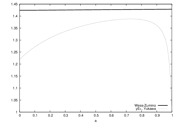
The exponent hardly depends on the cutoff parameter, and it agrees a little better with from Ref. \citenSynatschke:2010ub than of the Yukawa model.
Appendix E Integrals of a cutoff function
We define the following integrals:
| (121) |
For a particular choice of the cutoff function (see Fig. 10)
| (122) |
the above integrals can be evaluated easily as follows:
| (123) |

References
- [1] F. Gliozzi, J. Scherk, D. Olive, \NPB122,1977,253-290
- [2] C. Becchi, “On the construction of renormalized gauge theories using renormalization techniques,” hep-th/9607188
- [3] T. Morris, \PTPS131,1998,395-414
- [4] K.I. Aoki, \IJMPB14,2000,1249-1326
- [5] C. Bagnuls, C. Bervillier, \PR348,2001,91
- [6] J. Berges, N. Tetradis, C. Wetterich, \PR363,2002,223-386
- [7] J. Pawlowski, \ANN322,2007,2831-2915
- [8] H. Gies, “Introduction to the functional RG and applications to gauge theories,” hep-ph/0611146
- [9] B. Delamotte, “An introduction to the nonperturbative renormalization group,” cond-mat/0702365
- [10] Y. Igarashi, K. Itoh, H. Sonoda, \PTPS181,2010,1-166
- [11] O. Rosten, “Fundamentals of the Exact Renormalization Group,” arXiv:1003.1366[hep-th]
- [12] ERG2010 Conference, http://www.physics.ntua.gr/corfu2010/erg.html
- [13] J. Rudnick, \PRB18,1978,1406-1416
- [14] K. Wilson, J. Kogut, \PRP12,1974,75-200
- [15] B. Rosenstein, B. Warr, S. Park, \PRL62,1989,1433-1436
- [16] F. Synatschke, J. Braun, A. Wipf, \PRD81,2010,125001
- [17] L. Rosa, P. Vitale, C. Wetterich, \PRL86,2001,958-961
- [18] J. Polchinski, \NPB231,1984,269-295
- [19] M. Pernici, M. Raciti, \NPB531,1998,560-592
- [20] H. Sonoda, \JPA40,2007,5733-5750
- [21] J. Latorre, T. Morris, \JHEP0011,20000,004
- [22] D. Litim, \PLB486,2000,92-99
- [23] F. Wegner, A. Houghton, \PRA8,1973,401-412
- [24] P. Stevenson, \PRD23,1981,2916
- [25] P. Chaikin, T. Lubensky, Principles of Condensed Matter Physics (Cambridge University Press, 1995)
- [26] S. Hands, A. Kocic, J. Kogut, \PLB273,1991,111-117
- [27] S.-S. Lee, “TASI Lectures on Emergence of Supersymmetry, Gauge Theory and String in Condensed Matter Systems,” arXiv:1009.5127[hep-th]