Origin of Excess Low Energy States
in a Disordered Superconductor
in a Zeeman Field
Abstract
Tunneling density of states measurements of disordered superconducting (SC) Al films in high Zeeman fields reveal a significant population of subgap states which cannot be explained by standard BCS theory. We provide a natural explanation of these excess states in terms of a novel disordered Larkin-Ovchinnikov (dLO) phase that occurs near the spin-paramagnetic transition at the Chandrasekhar-Clogston critical field. The dLO superconductor is characterized by a pairing amplitude that changes sign at domain walls. These domain walls carry magnetization and support Andreev bound states that lead to distinct spectral signatures at low energy.
A central theme in condensed matter physics is the quest for new states of matter with unusual arrangements of interacting electrons, spins, and atoms. The interplay between superconductivity and magnetism is an especially rich source of interesting physics that gives rise to various types of exotic superconductors such as cuprates, pnictides, ruthenates, and heavy-fermion materials [1, 2]. There is also, however, the possibility of exotic superconductivity of a different type, which arises when a conventional BCS superconductor at low temperature is subjected to an external Zeeman field. In the simplest scenario, the superconductor undergoes a first-order transition into a polarized normal Fermi liquid [3, 4] when the Zeeman splitting becomes of the order of the superconducting gap at the Chandrasekhar-Clogston critical field . However, nature has a more intriguing way of resolving the tussle: the electrons can self-organize into a novel intermediate state known as a Fulde-Ferrell-Larkin-Ovchinnikov (FFLO) state near . [5, 6, 7, 8, 9, 10] An FFLO state consists of regions of positive and negative pairing amplitude separated by domain walls where the magnetization is piled up; it can be thought of as an “electronic liquid crystal,” an example of emergent microscale phase separation. Interest in FFLO physics crosses traditional boundaries between condensed matter, cold atomic gases[11], quantum chromodynamics[12], nuclear physics, and astrophysics[13], and there is currently an intense effort to search for FFLO phases in superconductors as well as in cold atoms[14].
Hitherto, only thermodynamic signatures of the FFLO phase have been reported, and these have been limited to a few layered organic superconductors and the heavy fermion material CeCoIn5 [15, 16, 17]. The realization of FFLO in traditional superconducting systems has been hampered by its sensitivity to disorder and spin-orbit scattering. Notwithstanding these issues, we show that even in the presence of disorder, where the fully coherent FFLO phase is suppressed, spectroscopic manifestations of FFLO fluctuations are readily observable.
Main results: We present density of states (DoS) calculations based on a disordered attractive Hubbard model, along with low-temperature tunneling DoS measurements on ultra-thin Al films. We show that, contrary to popular belief, FFLO physics is not completely washed out by disorder. In fact, over a significant range of Zeeman fields we find a disordered Larkin-Ovchinnikov (dLO) state characterized by bound states in domain walls and low-energy spectral weight, which provides a natural explanation of the experimental anomalies.[18] Our calculations self-consistently account for the disorder and allow the pairing amplitude to adjust to the disorder profile. The novel dLO phase is robust to variations in field and disorder, and imprints a unique signature in the low-energy DoS within the superconducting gap.
Experimental setup: In the present study planar tunnel junctions formed on 3 nm-thick Al films were used to extract the low temperature quasiparticle DoS. Aluminum has a well documented low spin-orbit scattering rate [20] and superconducting transition temperature K with a zero field gap mV in thin film form. [For sample preparation see supplement]. Measurements of resistance and tunneling were carried out on an Oxford dilution refrigerator using a standard dc four-probe technique. Magnetic fields of up to 9 T were applied using a superconducting solenoid. A mechanical rotator was employed to orient the sample in situ with a precision of . The films were moderately disordered with sheet resistances of the order of , well below the quantum of resistance for superconductivity .
Experimental results and comparison with standard BCS theory: We present measurements of the tunneling conductance of Al films, which is mainly proportional to the superconducting DoS at the low temperatures used. Figure 1 shows the bias dependence in a parallel field at , in which the BCS coherence peaks have been Zeeman-split by the applied field. Figure 1 shows the parallel-field dependence of the zero-bias tunneling conductance , which is zero in the conventional superconducting state () and constant in the normal state (); however, there is a significant tail in over a range of fields . The colored curves in Fig. 1 and 1 are obtained within homogenous BCS mean field theory by solving the Usadel equations for the disorder-averaged semiclassical Green’s functions together with the self-consistent equations for the uniform order parameter and the internal magnetic field. The parameters involved are the gap energy, spin-orbit scattering rate, the orbital depairing rate, and the antisymmetric Fermi-liquid parameter; they are determined by fits[21, 22] to full spectra as in Fig. 1.
The observed excess zero-bias conductance can have various origins. (i) Imperfect alignment: The inset of Fig. 1, shows at several alignment angles between the film plane and the applied field. It is evident that our alignment mechanism is precise enough to find parallel orientation within the limits of the sensitivity of the tunneling conductance to , the perpendicular field component. (ii) Junction leakage is ruled out because all of the junctions used in this study had a very low zero-bias conductance in zero field, at 100 mK. (iii) Material inhomogeneities: In principle could lead to broadened transitions, however, the zero-field gap in Al (and hence the nominal critical field ) varies by only over a very wide range of sheet resistance[23] and averaging over a distribution of gaps fails to explain the large range of over which is finite. (iv) Pair-breaking: These effects scale as , where is the normal state diffusivity and is the film thickness. For our films as is decreased from 3 nm to 2 nm, decreases by an order of magnitude, but hardly changes. Furthermore, recent tunneling measurements of Al-EuS bilayers have shown that a comparable is produced by an interface-induced exchange field, which is a pure Zeeman field with no orbital depairing effects. [24]

Disordered LO states and excess low-energy spectral weight: Having ruled out all the above explanations, we now argue that the anomalous excess zero-bias conductance at intermediate fields is an intrinsic property of the condensate due to the development of an exotic disordered Larkin-Ovchinnikov (dLO) phase with an inhomogeneous pairing amplitude and magnetization.
Our model consists of the attractive Hubbard Hamiltonian with a disorder potential and a Zeeman field,
| (1) |
where are hopping amplitudes (equal to , taken as the unit of energy) between nearest-neighbor sites and , is the number operator for fermions of spin index at site , is the average chemical potential, is the Zeeman field, and is the local pairwise Hubbard interaction. The disorder potential at each site is picked independently from a uniform distribution on . We calculate the local densities , pairing amplitude , and spin-dependent DoS within a fully self-consistent Bogoliubov-de Gennes (BdG) framework including all Hartree shifts (see supplement for details). A phase diagram for this system was obtained in Ref. 25; in this paper we focus on spectral features.
As illustrated in Fig. 2, if is restricted to be uniform, we find that the BCS- and normal-state free energies cross at , the critical field for the first-order Chandrasekhar-Clogston transition (here differs from due to the moderate value of ). However, if is allowed to be inhomogeneous, BdG calculations predict two transitions, at a lower critical field and an upper critical field . The intermediate state () has both a finite pairing amplitude and a finite magnetization.
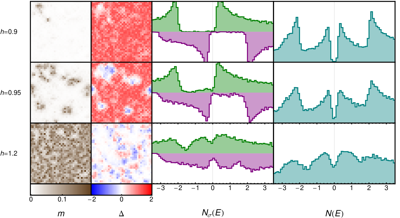
A physical understanding is provided in Fig. 3, which shows the local pairing amplitude , local magnetization , and spatially averaged DoS’s of up and down spins , for various values of . At low fields the system is a BCS superconductor with a nearly uniform order parameter , whose DoS contains coherence peaks at slightly broadened by inhomogeneous Hartree shifts[26, 27]. At high fields the system is normal (non-superconducting) with nearly uniform magnetization. At intermediate fields there is a disordered Larkin-Ovchinnikov (dLO) state with the following features: (1) There is a strong modulation of the pairing amplitude which changes sign between positive and negative values. The oscillations at wavevector are partially disrupted by the disorder potential. (2) The magnetization is finite in the domain walls where the pairing amplitude is small. (3) There is significant low-energy weight in the DoS, as illustrated in the rightmost column of Fig. 3. This is the main new result of this paper, and it is a likely explanation for the similar low-energy weight seen in experiments (Fig. 1).
Origin of low-energy states: When the Zeeman field exceeds a certain lower critical field, magnetization begins to penetrate the sample in the form of domain walls (brown regions in Fig. 4). The majority electrons are unable to enter the superconducting regions due to the gap, and so they are confined to the domain walls by Andreev reflection, forming Andreev bound states with a distribution of energies. Whereas in a clean LO state[28, 10] tunneling between domain walls gives rise to subgap bands, in a dLO state the bound states are likely to remain localized, but they still contribute to the low-energy DoS. Indeed, comparing Figs. 4(d) and (e) shows that the low-energy weight is concentrated in the same regions as the magnetization. The tunneling DoS (unlike transport measurements) is sensitive to local electronic structure, and hence the low-energy spectral signatures of LO should remain even when phase fluctuations prevent the development of long-range LO order.[29]
We conclude that dLO physics is a likely explanation of the longstanding mystery of excess zero-bias tunneling conductance of Al films near the spin-paramagnetic transition.[18] Our results suggest that the parallel-field-tuned[30, 31] superconductor-insulator transition (SIT) occurs via a dLO phase in which the gap is filled in by Andreev bound states. This scenario is distinct from the zero-field thickness-tuned “fermionic” SIT where the gap closes[32, 33, 34], and from the “bosonic” SIT [35, 26, 27, 36, 37] where the gap appears to remain finite across the SIT.
We acknowledge support from the U.S. Department of Energy, Office of Basic Energy Sciences, Division of Materials Sciences and Engineering under Awards DE-FG02-07ER46423 (YLL,NT) and DE-FG02-07ER46420 (PWA). GC is supported by Yale University.
References
- [1] J. Zaanen, et al., Nature Physics, 2, 138 (2006).
- [2] G. R. Stewart, Rev. Mod. Phys., 56, 755 (1984).
- [3] B. S. Chandrasekhar, Appl. Phys. Lett., 1, 7 (1962).
- [4] A. M. Clogston, Phys. Rev. Lett., 9, 266 (1962).
- [5] P. Fulde and R. A. Ferrell, Phys. Rev., 135, A550 (1964).
- [6] A. I. Larkin and Y. N. Ovchinnikov, Zh. Eksp. Teor. Fiz., 47, 1136 (1964), also Sov. Phys. JETP 20, 762 (1965).
- [7] K. Machida and H. Nakanishi, Phys. Rev. B, 30, 122 (1984).
- [8] H. Burkhardt and D. Rainer, Ann. Physik, 506, 181 (1994).
- [9] N. Yoshida and S.-K. Yip, Phys. Rev. A, 75, 063601 (2007).
- [10] Y. L. Loh and N. Trivedi, Phys. Rev. Lett., 104, 165302 (2010).
- [11] L. Radzihovsky and D. E. Sheehy, Rep. Prog. Phys., 73, 076501 (2010).
- [12] R. Casalbuoni and G. Nardulli, Rev. Mod. Phys., 76, 263 (2004).
- [13] M. Alford, J. A. Bowers, and K. Rajagopal, Phys. Rev. D, 63, 074016 (2001).
- [14] Y. A. Liao, et al., Nature, 467, 567 (2010).
- [15] H. A. Radovan, et al., Nature, 425, 51 (2003).
- [16] G. Koutroulakis, et al., Phys. Rev. Lett., 104, 087001 (2010).
- [17] Y. Yanase, New Journal of Physics, 11, 055056 (2009).
- [18] P. W. Adams, Phys. Rev. Lett., 92, 067003 (2004).
- [19] N. Trivedi, R. T. Scalettar, and M. Randeria, Phys. Rev. B, 54, R3756 (1996).
- [20] R. Meservey, P. M. Tedrow, and R. C. Bruno, Phys. Rev. B, 11, 4224 (1975).
- [21] G. Catelani, X. S. Wu, and P. W. Adams, Phys. Rev. B, 78, 104515 (2008).
- [22] G. Catelani, Y. M. Xiong, X. S. Wu, and P. W. Adams, Phys. Rev. B, 80, 054512 (2009).
- [23] W. Wu and P. W. Adams, Phys. Rev. Lett., 73, 1412 (1994).
- [24] Y. M. Xiong, S. Stadler, P. W. Adams, and G. Catelani, Phys. Rev. Lett., 106, 247001 (2011).
- [25] Q. Cui and K. Yang, Phys. Rev. B, 78, 054501 (2008).
- [26] A. Ghosal, M. Randeria, and N. Trivedi, Phys. Rev. Lett., 81, 3940 (1998).
- [27] A. Ghosal, M. Randeria, and N. Trivedi, Phys. Rev. B, 65, 014501 (2001).
- [28] M. R. Bakhtiari, M. J. Leskinen, and P. Törmä, Phys. Rev. Lett., 101, 120404 (2008).
- [29] L. Radzihovsky and A. Vishwanath, Phys. Rev. Lett., 103, 010404 (2009).
- [30] F. Zhou and B. Spivak, Phys. Rev. Lett., 80, 5647 (1998).
- [31] Y. Dubi, Y. Meir, and Y. Avishai, Nature, 449, 876 (2007).
- [32] V. F. Gantmakher and V. T. Dolgopolov, Physics-Uspekhi, 53, 1 (2010).
- [33] J. M. Valles, R. C. Dynes, and J. P. Garno, Phys. Rev. Lett., 69, 3567 (1992).
- [34] A. M. Finkel’stein, Physica B, 197, 636 (1994).
- [35] M. P. A. Fisher, P. B. Weichman, G. Grinstein, and D. S. Fisher, Phys. Rev. B, 40, 546 (1989).
- [36] K. Bouadim, Y. L. Loh, M. Randeria, and N. Trivedi, arXiv:1011.3275.
- [37] H. Q. Nguyen, et al., Phys. Rev. Lett., 103, 157001 (2009).
Mystery of Excess Low Energy States
in a Disordered Superconductor
in a Zeeman Field:
Supplementary Information
I Sample Preparation
In the present study tunnel junctions were formed by first depositing a 3 nm thick Al film e-beam deposition of 99.999% Al stock onto fire polished glass microscope slides held at 84 K. After deposition, the film was exposed to the atmosphere for 10-20 minutes in order to allow a thin native oxide layer to form. Then a non-superconducting Al counterelectrode was deposited from an Al 2024 alloy target, with the oxide serving as the tunneling barrier. The low temperature parallel critical fields of the counter-electrodes were 6 T, in good agreement with the expected . The junction area was about 1 mm1 mm, while the junction resistance ranged from 15-100 k depending on exposure time and other factors. Only junctions with resistances much greater than that of the films were used, in order to be in the tunneling regime.
II Variational Bogoliubov-de Gennes Method
The combination of the Zeeman field and the disorder potential ultimately leads to inhomogeneous, spin-dependent Hartree potentials. Therefore, we use a generalized Bogoliubov-de Gennes (BdG) method[1] in which all BdG eigenvalues and eigenvectors are distinct (where is the number of sites).
For convenience, we write the Hamiltonian in terms of an applied chemical potential (where is the quenched random potential) and field at every site:
| (1) |
where are densities with respect to half-filling and represents attraction.
We decouple the Hubbard interaction in charge, spin, and pairing channels. It is difficult to justify a traditional derivation of the self-consistent BdG equations with multiple-channel decoupling, because this appears to overcount the interaction term. We have performed a rigorous derivation based on the variational formalism.[2] In this approach, we postulate a trial Hamiltonian , which defines a trial density matrix , and we then minimize the variational free energy [given in Eq. (9)] with respect to the variational parameters: the Hartree chemical potential , Hartree field , and self-consistent pairing field . This formalism has the practical advantage that can be used to assess the quality of the variational approximation during the approach to self-consistency, and that it provides a rigorous upper bound to the true free energy. Our implementation is as follows:
- 1.
Make arbitrary initial guesses for the Hartree chemical potential , Hartree field , and self-consistent pairing field at every site . These constitute a set of real-valued variational parameters.
- 2.
Find the effective chemical potential and effective field at every site. These effective potentials include both the applied potentials and the Hartree potentials (resulting from the decoupling of the term); they enter the mean-field Hamiltonian,
(2) - 3.
Construct the Hamiltonian matrix , where the indices distinguish between up-particle and down-hole sectors connected by matrix elements :
(3) - 4.
Diagonalize to obtain eigenvalues and eigenvectors , where the eigenmode index runs from to . (These eigenvectors are generalizations of the and vectors that appear in the original BdG formalism.)
- 5.
Find the symmetrized occupation numbers .
- 6.
Compute the number densities (relative to half-filling) and the pairing density at every site :
(4) (5) (6) and thence the number density and magnetization on each site,
(7) (8) - 7.
Compute the variational free energy
(9) - 8.
According to the usual variational principle, we wish to minimize with respect to , , and (to obtain a least upper bound to the true free energy). In practice this can be done by solving the stationarity condition , i.e., finding a root of the -dimensional equation
(10) where is the vector of variational parameters and
(11) is the residual vector (the “distance” from self-consistency). We use the standard Broyden method,[3] which is a superlinearly convergent quasi-Newton method for multidimensional root-finding. The first iteration of the Broyden procedure is equivalent to fixed-point iteration of the self-consistency equations
(12) (13) (14) We also inspect to verify that the root of Eq. (10) corresponds to a minimum of Eq. (9), and not to a maximum. We restart the Broyden method using Eq. (14) if a Broyden step results in a large increase in (since quasi-Newton methods are prone to instability).
After convergence we calculate further quantities, including the densities of states for up and down electrons (which are the main point of interest in this paper):
| (15) |
References
- [1] P. G. de Gennes, Superconductivity in Metals and Alloys, Benjamin, New York (1966).
- [2] P. M. Chaikin and T. C. Lubensky, Principles of Condensed Matter Physics, Cambridge University Press, Cambridge (2000).
- [3] W. H. Press, B. P. Flannery, S. A. Teukolsky, and W. T. Vetterling, Numerical Recipes in FORTRAN 77: The Art of Scientific Computing, Cambridge University Press, 2 edition (1992).