Holography of charged dilatonic black branes at finite temperature

Mariano Cadoni Email: email: mariano.cadoni@ca.infn.it Affiliation: Dipartimento di Fisica, Università di Cagliari and INFN, Sezione di Cagliari - Cittadella Universitaria, 09042 Monserrato, Italy. Paolo Pani Email: email: paolo.pani@ist.utl.pt Affiliation: CENTRA, Departamento de Física, Instituto Superior Técnico, Universidade Técnica de Lisboa - UTL, Av. Rovisco Pais 1, 1049 Lisboa, Portugal.

August 24, 2026

Abstract

We investigate bulk and holographic features of finite-temperature black brane solutions of 4D anti-de Sitter Einstein-Maxwell-dilaton-gravity (EMDG). We construct, numerically, black branes endowed with non trivial scalar hairs for broad classes of EMDG. We consider both exponential and power-law forms for the coupling functions, as well as several charge configurations: purely electric, purely magnetic and dyonic solutions. At finite temperature the field theory holographically dual to these black brane solutions has a rich and interesting phenomenology reminiscent of electron motion in metals: phase transitions triggered by nonvanishing VEV of scalar operators, non-monotonic behavior of the electric conductivities as function of the frequency and of the temperature, Hall effect and sharp synchrotron resonances of the conductivity in presence of a magnetic field. Conversely, in the zero temperature limit the conductivities for these models show a universal behavior. The optical conductivity has a power-law behavior as a function of the frequency, whereas the DC conductivity is suppressed at small temperatures.

I Introduction

One of the most productive applications of the AdS/CFT [1] correspondence is obtained when one considers the regime in which the classical gravity approximation is reliable. In this regime we can deal with strongly coupled quantum field theories (QFTs) in $d-1$ dimensions by investigating classical gravity in $d$ dimensions. In particular, this holographic approach has been recently used to provide techniques for the computation of thermodynamical and transport properties of strongly interacting quantum field theories, which could be relevant in the description of condensed matter phenomena [2, 3, 4, 5].

The basic structure of the holographic correspondence is given by a black hole (black brane) in the $d$ -dimensional bulk, which is holographically dual to a thermal QFT in $d-1$ dimensions. This framework has been used in several cases to investigate the hydrodynamical limit of the QFT, to compute spectral functions and so on. However, the most interesting results come up when we consider a thermal QFT with finite charge density, i.e a charged black hole in the bulk. An even richer structure is obtained if we include in the bulk a charged scalar field with a minimal (covariant) coupling to the gauge potential. Below a critical temperature the bulk theory allows for solutions with a non-trivial profile of the scalar field. This corresponds to the formation of a charged condensate in the dual theory that breaks spontaneously a global $U(1)$ symmetry. The new phase is therefore characterized by phenomena typical of superfluid or superconducting systems, as one can show by using the basic rules of the AdS/CFT correspondence, i.e by studying the response of small perturbations of the black hole background [6, 7, 8].

This general idea of holographic superconductor has generated in the last couple of years a flurry of activity on AdS gravity whose holographic QFT duals have transport features with a metal or metal-like behavior [9, 10, 11, 12, 13, 14, 15, 16, 17].

Most of the efforts for understanding the holography of charged black branes have focused on the case of AdS Einstein-Maxwell gravity with a charged scalar fields minimally coupled to the electromagnetic field. However, there are several reasons for extending the investigation to the case in which the scalar is non-minimally coupled to the $U(1)$ field, the so called Einstein-Maxwell-dilaton gravity (EMDG): $1)$ Non-minimal couplings of the form $f(\phi)F^{2}$ between a scalar fields $\phi$ and the Maxwell tensor are very common in supergravity and in the low-energy effective action of string theory models. $2)$ Exact, charged dilaton black hole solutions with AdS asymptotics are known in some cases, for instance the family of four-charge black holes in ${\cal N}=8$ four-dimensional gauged supergravity [18]. $3)$ Charged black brane solutions with AdS asymptotics of EMDG have a rather interesting thermodynamical phase structure [19, 20, 21]. For instance, when the coupling function $f$ satisfies the requirement $f^{\prime}(0)=0$ the model allows for a phase transition between the Reissner-Nordstrom (RN) black brane and a charged black brane endowed with a scalar hair [19], corresponding in the dual field theory to the formation of a scalar condensate. $4)$ In the few cases in which EMDG has been investigated within the holographic perspective, the models have shown a rather rich and interesting phenomenology [22, 23, 19, 24, 25, 26, 27, 28, 29]. $5)$ Finally, the black brane solutions of EMDG are good candidates for gravitational backgrounds holographically dual to Lifshitz-like theories [23, 30, 31, 32].

Until now investigations of charged dilaton AdS black branes and their holographic features have considered almost exclusively the cases of coupling functions $f(\phi)$ with exponential behavior in the zero temperature limit [23, 20, 32]. In this paper we extend the investigation of the black brane solutions of EMDG in four dimensions (4D) and of their holographic properties. On the one hand we complete the investigation of EMDG with exponential coupling $f\sim e^{\alpha\phi}$ , by considering electrically charged solutions of the model at finite, nonvanishing, temperature. On the other hand, we extend the investigation to electrically charged black brane solutions of models with a power-law coupling function $f\sim\phi^{m}$ both at finite temperature and in the zero temperature limit. Last but not least, we consider dyonic solutions of models characterized by $f^{\prime}(0)=0$ , thus allowing a phase transition between the dyonic RN solution and a dyonic black brane with a nontrivial scalar hair.

After constructing, numerically, the black brane solutions endowed with scalar hairs for our models, we investigate, using the AdS/CFT correspondence, the field theory holographically dual to these black brane solutions both at finite temperature and in the zero temperature limit. We show that at finite temperature the dual field theory presents a rich phenomenology: phase transitions triggered by nonvanishing VEV of scalar operators, non-monotonic behavior of the electric conductivities, Hall effect and sharp synchrotron resonances of the conductivity in presence of a magnetic field. On the other hand, in the zero temperature limit the optical conductivity for these models shows a universal power-law behavior as a function of the frequency, whereas the DC conductivity is suppressed at small temperature and in general scales as $T^{2}$ .

Our investigations suggest an intriguing holographic picture for the black brane solutions of EMDG. We have an interpolation between some features of electron motion in metals at finite temperature and an universal strong repulsion behavior, characteristic of charged plasmas, at zero temperature.

The plan of the work is the following. In Sect. II we present general models of EMDG and the equations of motion. Sect. III is devoted to the study of electrically charged dilatonic black branes in these models and their holographic properties at finite temperature. The zero temperature limit is discussed in Sect. IV. In Sect. V we discuss dyonic dilatonic black branes at finite temperature, while in Appendix A we briefly present purely magnetic solutions. Finally, we draw our conclusion in Sect. VI.

II Einstein-Maxwell-dilaton gravity in Anti de Sitter spacetime

In this paper we will consider general models of EMDG in 4D, which is described by the action

S=\int d^{4}x\sqrt{-G}\,{\cal L}=\int d^{4}x\sqrt{-G}\left(R-\frac{f(\phi)}{4}F^{2}-\frac{1}{2}\partial^{\mu}\phi\partial_{\mu}\phi-V(\phi)\right)\,,

(1)

where $\phi$ is a scalar field (the dilaton) and $F$ is the field strength for the Maxwell field. The model is parametrized by two functions: the coupling $f(\phi)$ between the scalar and the Maxwell tensor and the potential $V(\phi)$ describing the self-interaction of the scalar. Non-minimal couplings, $f(\phi)F^{2}$ between a scalar fields $\phi$ and the Maxwell tensor emerge naturally in supergravity and in the low-energy effective action of string theory.

In asymptotically flat spacetime, exact, charged black holes (or black branes) solutions of EMDG carrying non trivial scalar hairs (i.e. different from the usual Reissner-Nordstrom (RN) solutions) are known since a long time [33, 34, 35, 36, 37]. These solutions involve a non-constant scalar field and differ from the RN black hole both with respect to the causal structure of the spacetime and to the thermodynamical behavior. Conversely, for charged dilaton black holes with AdS asymptotics exact solutions with scalar hairs are known only in few cases [18, 38], the most important one being represented by the family of four-charge black holes in ${\cal N}=8$ four-dimensional gauged supergravity [18].

In recent years there has been a renewed interest for black hole solutions of EMDG with AdS asymptotics. This interest has been triggered by the gauge/gravity duality [1, 39] and by the search for gravitational duals of strongly coupled condensed matter systems with finite charge density [2, 3, 4].

However, until now the investigation of charged dilaton AdS black holes and their holographic features has been almost completely restricted to case of coupling functions $f(\phi)$ with exponential behavior [23, 19, 20] and to electric charged solutions (see however Ref. [24]). There are several reasons behind this choice. Exponential coupling functions $f(\phi)$ are rather natural in low-energy effective string theory. Furthermore, it is very difficult to find exact solutions of generic AdS Maxwell-dilaton gravity and typically one has to resort to numerical calculation. Conversely, an exponential form for $f(\phi)$ enables one to find exact solutions at least in the extremal limit, where they take a Lifshitz-like form [23].

Although the pure exponential form $f(\phi)=e^{\alpha\phi}$ does not allow for a RN solution, simple deformations preserving an exponential behavior on the horizon, such as $f(\phi)=\cosh{\alpha\phi}$ , do allow for it. The coexistence in the model of the RN solution together with solutions with scalar hairs is crucial for having a phase transition [19].

In this paper we will not limit ourself to the case of exponential coupling functions $f(\phi)$ but we will extend our investigation to the black brane solutions in a broad class of EMDG models.

The equations of motion stemming from the action (1) read

	$\displaystyle\nabla_{\mu}\left(f(\phi)F^{\mu\nu}\right)=0\,,$
	$\displaystyle\nabla^{2}\phi=\frac{dV(\phi)}{d\phi}+\frac{df(\phi)}{d\phi}\frac{F^{2}}{4}\,,$		(2)
	$\displaystyle R_{\mu\nu}-\frac{1}{2}G_{\mu\nu}R=\frac{f(\phi)}{2}\left(F_{\mu\rho}F_{\nu}^{\rho}-\frac{G_{\mu\nu}}{4}F^{\rho\sigma}F_{\rho\sigma}\right)+\frac{1}{2}\left(\partial_{\mu}\phi\partial_{\nu}\phi-\frac{G_{\mu\nu}}{2}\partial^{\rho}\phi\partial_{\rho}\phi\right)-\frac{G_{\mu\nu}}{2}V(\phi)\,.$

We will look for static solutions of the previous equations with translational symmetry in two spatial directions (black branes) carrying electric and/or magnetic charges. The metric and the scalar field have the form

ds^{2}=-g(r)e^{-\chi(r)}dt^{2}+\frac{dr^{2}}{g(r)}+r^{2}(dx^{2}+dy^{2})\,,\qquad\phi=\phi(r).

(3)

Since we are interested in the holographic features of our models, we will only constrain the form of the coupling functions $f(\phi)$ and $V(\phi)$ by imposing conditions at $r=\infty$ (corresponding to the UV region of the dual field theory) and at the horizon of the extremal, zero temperature, solution (corresponding to the IR region of the dual field theory).

We first require the solutions to be asymptotically AdS and the potential $V(\phi)$ to allows for stable AdS vacua. Assuming for simplicity that $V(\phi)$ has only one extremum, we can consider without loss of generality that $\phi=0$ as $r\to\infty$ . The potential can be now expanded for small values of the field as¹¹ 1 The easiest way to include a massive scalar field is by considering $V(\phi)=-{6}/{L^{2}}+{\beta}/(2L^{2})\phi^{2}$ . Although the numerical results presented in this paper where obtained using this form of $V(\phi)$ , other choices give qualitatively similar results, provided they satisfy Eq. (4). We explicitly checked that the potential $V(\phi)=-{6}/{L^{2}}\cosh(\phi/\sqrt{3})$ gives the same qualitative results as the polynomial form with $\beta=-2$ .

V(\phi)=-\frac{6}{L^{2}}+\frac{\beta}{2L^{2}}\phi^{2}+{\cal O}(\phi^{3})\,,

(4)

where $L$ is the AdS radius and $\beta$ parametrizes the mass of the scalar field, $m_{s}^{2}L^{2}=\beta$ . The AdS vacuum is stable if the mass parameter satisfies the Breitenlohner-Freedman (BF) bound $\beta\geq-9/4$ [40]. On the other hand the coupling functions $f(\phi)$ is only constrained by $f(0)=1$ ²² 2 In general, we should only require $f(0)$ to be finite, however $f(0)$ can be set to the unit by a redefinition of the charges.. Notice that in general we will not require the AdS-RN black hole to be a solution of the equations (2). This would imply the additional condition $f^{\prime}(0)=0$ .

Secondly, in the extremal limit (the zero temperature solution) we can assume without loss of generality that the horizon is located at $r=0$ . The IR behavior of the field theory dual to our dilaton gravity model will be determined by the asymptotic expansion of the solution near $r=0$ . Because in the near-horizon region we expect this dual theory to be strongly coupled, we assume that $\phi\to\infty$ as $r\to 0$ and $f(\infty)=\infty$ . The asymptotic form of the functions $f(\phi)$ and $V(\phi)$ is therefore determined by the leading term in the $\phi\to\infty$ expansion of the field.

The class of functions $f(\phi)$ and $V(\phi)$ satisfying the requirements above is rather broad. However, we will not expect the qualitative behavior of the dual field theory to depend strongly on the details of the functional form of $f(\phi)$ and $V(\phi)$ . The essential information is contained, for what concerns the UV region, in $V^{\prime\prime}(0)$ , $f^{\prime}(0)$ and $f^{\prime\prime}(0)$ (primes denote derivative with respect to $\phi$ ). On the other hand the form of the potential $V(\phi)$ seems to be quantitatively but not qualitatively relevant for the description of the zero temperature extremal limit [23, 19]. Thus, the behavior in the IR region will be determined by the leading terms in the $\phi\to\infty$ expansion of $f(\phi)$ . Obviously, the most interesting cases are represented by an exponential $f\sim e^{\alpha\phi}$ and a power-law $f\sim\phi^{m}$ behavior.

A vanishing value of $f^{\prime}(0)$ discriminates between models for which a phase transition between the AdS-RN black brane and a solution with scalar hairs is possible. The values of $V^{\prime\prime}(0)$ , and $f^{\prime\prime}(0)$ determine both the parameter region where the phase transition takes effectively place and the specific behavior of the transport coefficients of the dual theory [19].

It follows that a rough classification of the Maxwell-dilaton-gravity model with interesting holographic features can be simply given in terms of a vanishing/nonvanishing $f^{\prime}(0)$ and by the leading terms in the $\phi\to\infty$ expansion of $f(\phi)$ .

Electric charged solutions for models with $f^{\prime}(0)=0$ , both at finite and zero temperature, has been investigated in Ref. [19]. Models with exponential coupling function $f(\phi)$ have been investigated in the zero temperature limit $T=0$ both in the case of electric and dyonic solutions [23, 24].

In this paper we complete the investigation of the holographic properties of the most interesting EMDG models, by considering:
$a)$ Electrically charged solutions of models with $f\sim e^{\alpha\phi}$ at finite temperature ;
$b)$ Electrically charged solutions of models with $f\sim\phi^{m}$ ( $m\neq 1$ ) both at finite temperature and in the zero temperature limit;
$c)$ Electrically charged solutions of models with $f\sim\phi$ both at finite temperature and in the zero temperature limit
$d)$ Dyonic solutions of models with $f^{\prime}(0)=0$ .

Notice that we consider separately the power-law case and the linear case. This is because the former case allows for a phase transition to the AdS-RN solution ( $f^{\prime}(0)=0$ ), whereas the latter does not ( $f^{\prime}(0)\neq 0$ ).

III Electrically charged dilatonic black branes at finite temperature

In this section we derive, numerically, electrically charged black brane solutions of the EMDG (1) at finite temperature with exponential, power-law and linear coupling and investigate their holographic features.

Since only the $A_{0}$ component of the gauge potential is non-vanishing and $\phi=\phi(r)$ , the equations of motion (2) become

$\displaystyle\phi^{\prime\prime}+\left(\frac{g^{\prime}}{g}-\frac{\chi^{\prime}}{2}+\frac{2}{r}\right)\phi^{\prime}(r)-\frac{1}{g}\frac{dV}{d\phi}+\frac{{A_{0}^{\prime}}^{2}e^{\chi}}{2g}\frac{df}{d\phi}$	$\displaystyle=$	$\displaystyle 0\,,$
$\displaystyle(r^{2}e^{\frac{\chi}{2}}f(\phi)A_{0}^{\prime})^{\prime}$	$\displaystyle=$	$\displaystyle 0\,,$
$\displaystyle\chi^{\prime}+\frac{r{\phi^{\prime}}^{2}}{2}$	$\displaystyle=$	$\displaystyle 0\,,$
$\displaystyle\frac{{\phi^{\prime}}^{2}}{4}+\frac{{A_{0}^{\prime}}^{2}e^{\chi}f(\phi)}{4g}+\frac{g^{\prime}}{rg}+\frac{1}{r^{2}}+\frac{V(\phi)}{2g}$	$\displaystyle=$	$\displaystyle 0\,,$	(5)

where now the prime denotes a derivative with respect to $r$ . Charged dilatonic black branes (CDBBs) solutions of the field equations (5) at finite temperature can be computed numerically by using the method discussed in Ref. [19] with slight modifications due to the form of $f(\phi)$ .

III.1 Numerical solutions

The numerical procedure for solving the field equations (5) consists essentially in three steps (see Ref. [19] for details). First, we characterize the solutions in terms of the behavior of the fields near the AdS boundary at $r=\infty$ and near the horizon at $r=r_{h}$ . Near the AdS boundary the solutions are specified by four parameters: the chemical potential $\mu$ , the charge density $\rho$ appearing in the expansion of the gauge potential $A_{0}=\mu-\rho/r$ , the black brane mass $M$ and the expectation values for the operators dual to the scalar field ${\cal O}_{-}$ , ${\cal O}_{+}$ . These are determined in terms of the asymptotic expansion of the scalar field³³ 3 In order to describe states of the dual field theory with a non vanishing expectation value for the operator dual to the scalar field, the asymptotic expansion $(\ref{bc_scalarB})$ should contain only normalizable modes [41]. When $m^{2}L^{2}\geq-5/4$ this requires the boundary condition ${\cal O}_{-}=0$ , whereas, when $-9/4<m^{2}L^{2}<-5/4$ two distinct choices are possible [42]: ${\cal O}_{-}=0$ or ${\cal O}_{+}=0$ . Finally, when the Breitenlohner-Freedman (BF) bound [40] is saturated, $m^{2}L^{2}=-9/4$ , the asymptotic behavior has a logarithmic branch, whose coefficient is required to vanish.:

\displaystyle\phi\sim\frac{{\cal O}_{-}}{r^{\Delta_{-}}}+\frac{{\cal O}_{+}}{r^{\Delta_{+}}}\,,\qquad\Delta_{\pm}=\frac{3\pm\sqrt{9+4\beta}}{2}\,.

(6)

Near the horizon the solutions are completely specified by four parameters: the horizon radius $r_{h}$ , $A_{0}^{\prime}(r_{h})$ , $\chi(r_{h})\equiv\chi_{h}$ and $\phi(r_{h})\equiv\phi_{h}$ . The black brane temperature $T$ can be expressed in terms of these parameters. Secondly, we reduce the numbers of parameters exploiting the scaling symmetries of the equations of motion. Using these symmetries the number of independent parameters specifying the solutions can be effectively reduced to two. Furthermore, we choose one of the independent parameters at the horizon such that either ${\cal O}_{-}=0$ or ${\cal O}_{+}=0$ . This is enough to describe the solution in terms of a single parameter.

Finally, we integrate numerically the equations of motion from the horizon to the AdS asymptotics, using a shooting method to impose either ${\cal O}_{-}=0$ or ${\cal O}_{+}=0$ . The result of this integration is a one-parameter family of solutions, the parameter being the black brane temperature.

We shall directly focus on the results of the numerical integration for the various models under consideration, referring to Ref. [19] for further details on the numerical technique used.

III.1.1 Exponential coupling function

Charged black branes solutions of dilaton gravity with an exponential coupling function at $T\sim 0$ have been recently studied in great detail in Refs. [23, 24]. Here we consider the solution at finite temperature and focus on models defined by

\displaystyle f(\phi)=e^{\alpha\phi}\,,\qquad V(\phi)=-\frac{6}{L^{2}}+\frac{\beta}{2L^{2}}\phi^{2}\,.

(7)

The model discussed in Ref. [23] is obtained for $\beta=0$ . We are interested in finite temperature effects for a generic mass of the scalar field.

Models with coupling functions given by Eqs. (7) do not allow for AdS-RN black branes, which may be regarded has a pleasant feature, since the large entropy of extremal AdS-RN black holes poses some problems of interpretation from the holographic perspective. Conversely, CCBBs have a vanishing entropy in the extremal limit. Moreover, they exist at any temperature, since no phase transition occurs in these models.

Our method provides numerical solutions for CDBBs at finite temperature. They describe hairy black branes, i.e. black branes endowed with a non trivial configuration for the scalar field $\phi$ . These hairy solutions can be completely characterized in terms of the expectation value of one of the neutral boundary operators ${\cal O}_{\pm}$ (the scalar condensate) defined in Eq. (6) as a function of the black hole temperature $T$ .

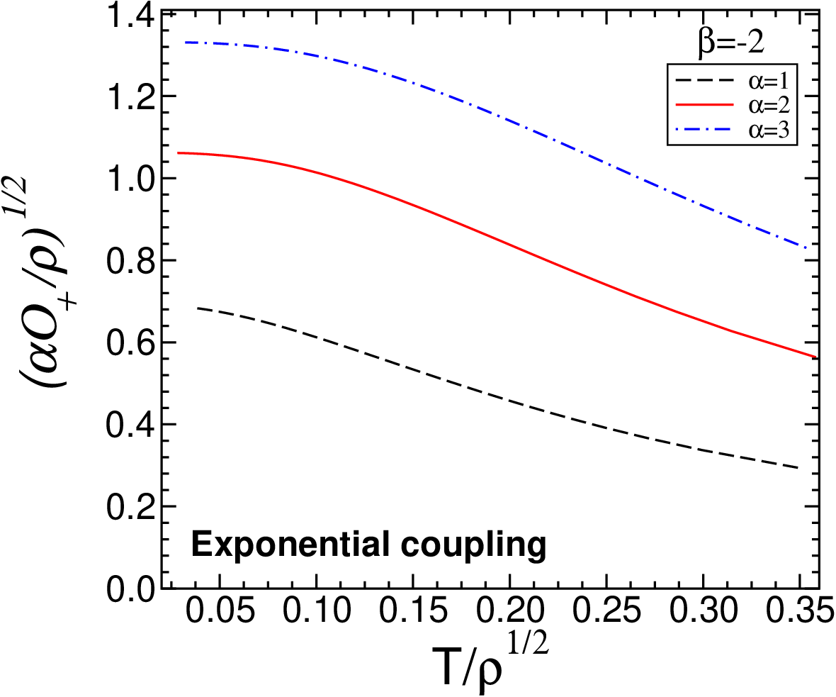
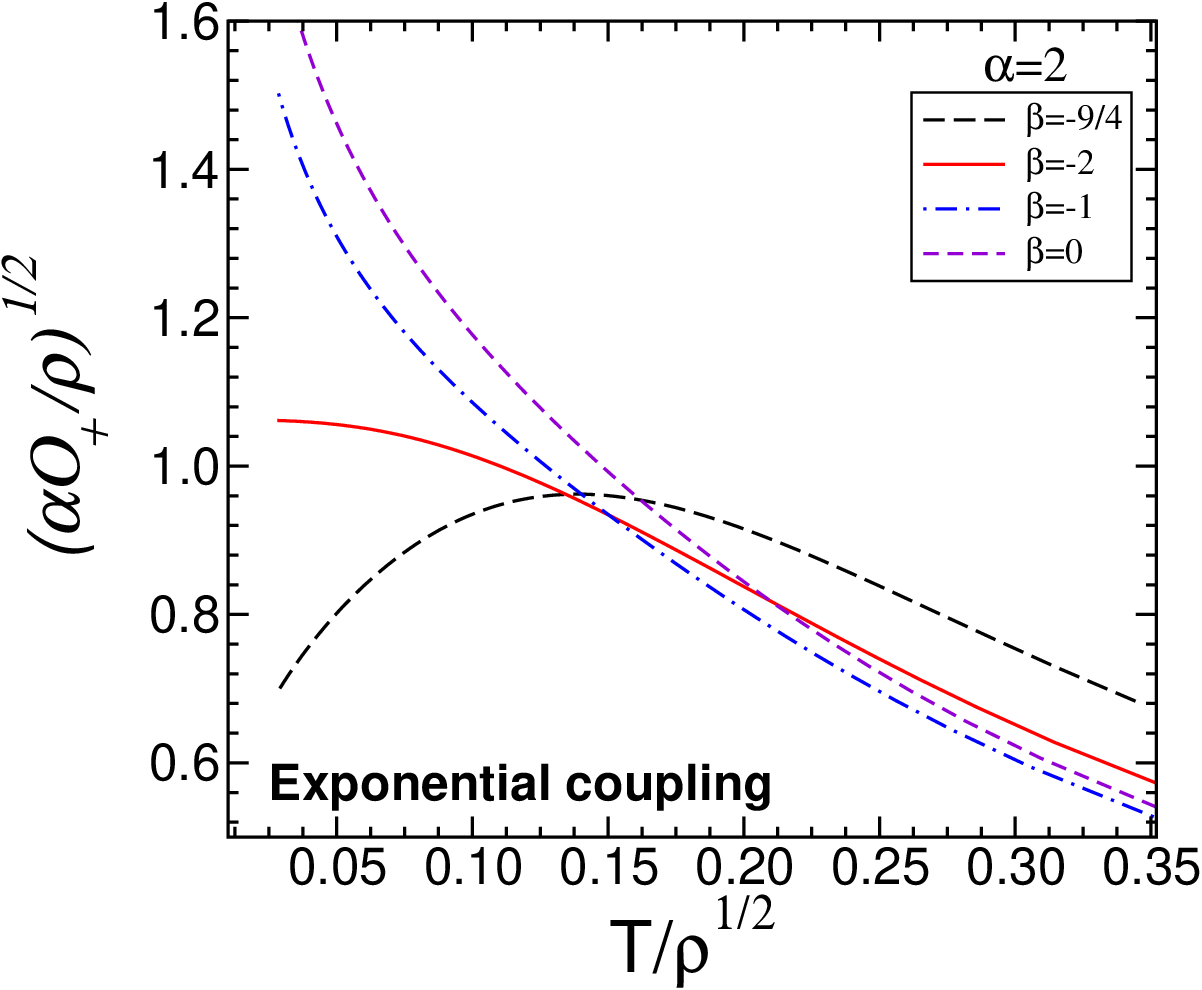
The behavior of some of these boundary operators as function of $T$ are shown in the upper panels of Fig. 1 for several values of $\alpha$ and $\beta$ .

Refer to caption — Figure 1: The scalar operator ${\cal O}_{+}$ as a function of the temperature for several values of $\alpha$ when $\beta=-2$ (left panels) and several values of $\beta$ when $\alpha=2$ (right panels). In the upper panels and lower panels we have used models with $f(\phi)=e^{\alpha\phi}$ and with linear coupling $f(\phi)=1+\alpha\phi$ , respectively. Results are qualitatively similar in the two cases.

The dependence of the condensate from $\alpha$ is quite simple. Roughly speaking, larger values of $\alpha$ shift the condensate up. However, the dependence on the mass $m_{s}$ of the scalar is more involved. In fact, the condensate monotonically depends on the temperature for $\beta=0,-1,-2$ , but it is a non-monotonic function in the BF limit, $\beta=-9/4$ . Notice that the condensate exists at any temperature and, although not shown in Fig. 1, it vanishes asymptotically when $T\gg\sqrt{\rho}$ .

III.1.2 Linear coupling function

Let us now consider a linear coupling function $f(\phi)$ and the usual self-interaction potential

f(\phi)=1+\alpha\phi\,,\qquad V(\phi)=-\frac{6}{L^{2}}+\frac{\beta}{L^{2}}\phi^{2}\,.

(8)

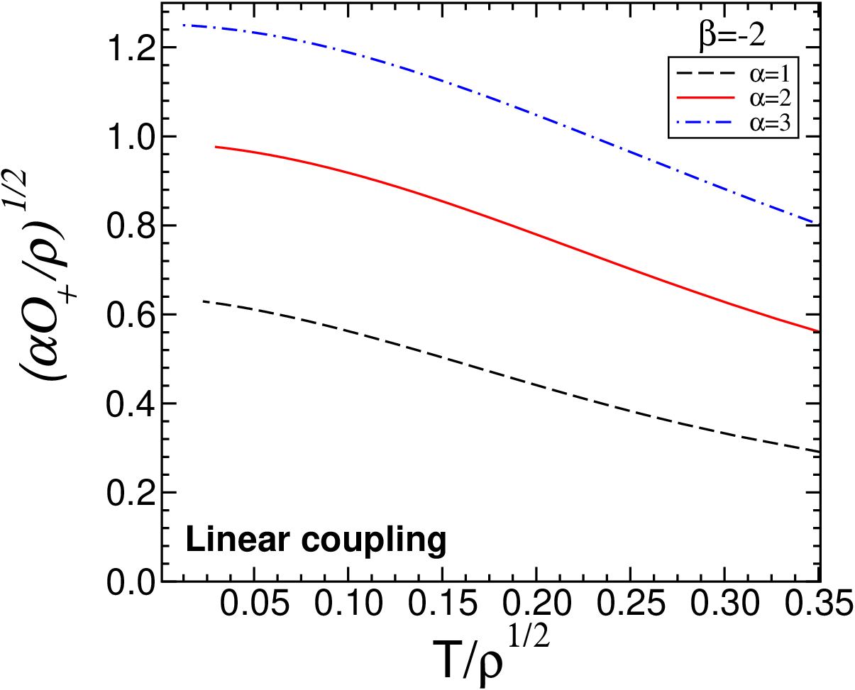
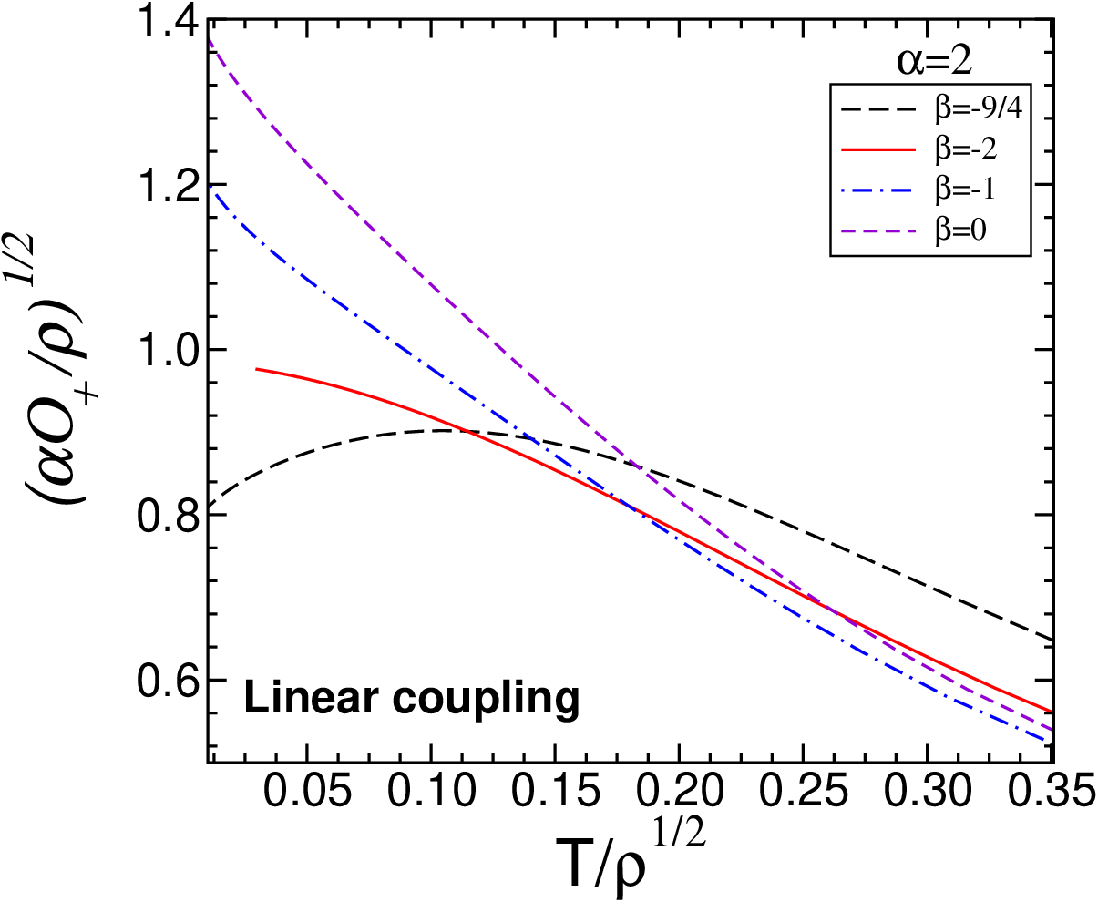
Similarly to the exponential case discussed in section (III.1.1), also here we have $f^{\prime}(0)\neq 0$ , forbidding the existence of AdS-RN solutions. Thus only hairy black hole solutions characterized by a nonvanishing scalar condensate are allowed. Because the coupling function $f(\phi)$ given by Eq. (8) is just the linear approximation near $\phi=0$ of the exponential coupling (7), these solutions have the same $r\to\infty$ behavior as those discussed in section (III.1.1). Obviously the two sets of solutions differ in the near-horizon region. The behavior of the scalar condensate is shown in the lower panels of Fig. 1 and it behaves in a way which is qualitatively similar to that described in the upper panels for exponential couplings. This suggests that the salient properties of these solutions are simply captured by the condition $f^{\prime}(0)\neq 0$ .

III.1.3 Power-law coupling function

The method described above can be also used to construct numerical solutions for the class of models with power-law coupling function,

f(\phi)=1+\alpha\phi^{m}\,,\quad m>1\,,\qquad V(\phi)=-\frac{6}{L^{2}}+\frac{\beta}{L^{2}}\phi^{2}\,.

(9)

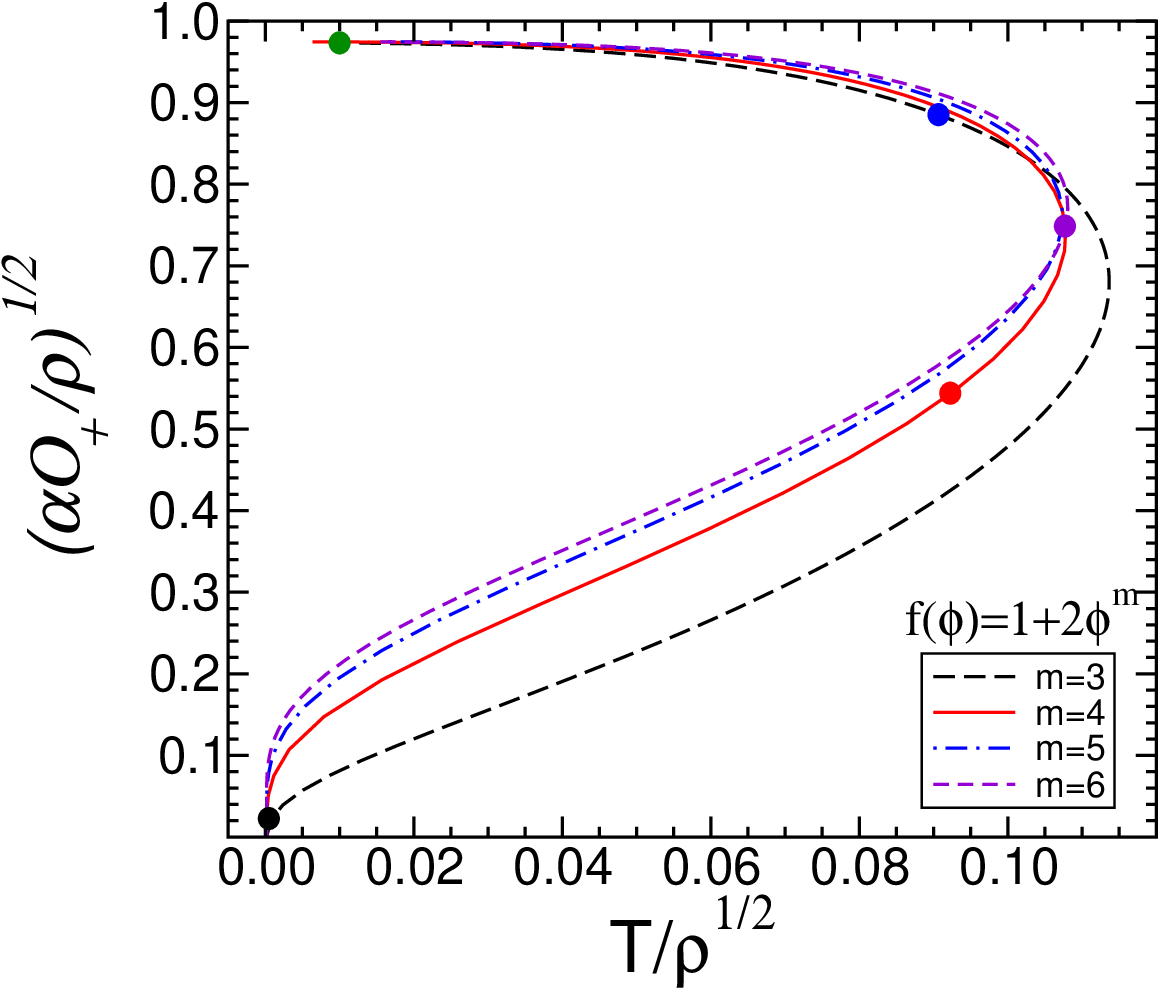
The most important difference between this and the previously discussed cases is that $f^{\prime}(0)=0$ . This implies that in these models black brane solutions with non trivial scalar profile for the scalar field can coexist with the AdS-RN black brane for any $m>1$ . In general, these models will be therefore characterized by a phase transition. Below a critical temperature $T_{c}$ the AdS-RN solution becomes unstable and the operator dual to the scalar field acquires a nonvanishing expectation value, i.e. a scalar condensate forms. This behavior is very similar to that observed in the class of models investigated in Ref. [19]. In the left panel of Fig. 2 we show the expectation value for the scalar operator ${\cal O}_{+}$ as a function of the temperature for different values of $m$ . Interestingly, near the critical temperature these solution exist also for $T>T_{c}$ and, for a given temperature, there exist two branches of solutions. This is due to a non-monotonic behavior of the function $T(\phi_{h})$ .

Moreover, as shown in the right panel of Fig. 2, in the first branch the hairy dilatonic solutions have always a larger free energy than the corresponding AdS-RN black brane at the same temperature. Hence, they are energetically less favored and likely decay into AdS-RN black branes. On the other hand, solutions in the second branch are unstable with respect to the AdS-RN solution only at (relatively) high values of $T$ . After the turning point shown in the right panel of Fig. 2, the difference in the free energy $\Delta F$ changes sign and solutions in the second branch are energetically favored all the way down to the zero temperature limit (see Ref. [43] for similar effects in models of holographic superconductors with nonminimal couplings). This behavior has to be compared with that arising in the EMDG models investigated in Ref. [19] (and also in the case of a scalar with covariant coupling with the gauge field [6, 7, 8]). In these latter cases the hairy solution exists and, it is stable, only below the critical temperature. Above $T_{c}$ only the AdS-RN solution exists [19, 6, 7, 8].

As we will discuss in detail in Sect. IV, in the zero temperature limit the hairy solutions are stable and show a behavior which is largely independent from the parameters. Indeed, the qualitative behavior does not depends on $m$ , $\alpha$ and $\beta$ . This universality can be traced back to the common property of these theories, which have $f^{\prime}(0)=0$ regardless of the values of $m$ and $\alpha$ .

III.2 Holographic properties

Holographic properties of CDBBs with exponential coupling function $f\sim\exp(\alpha\phi)$ have been investigated in great detail in Refs. [23, 24], in the zero temperature limit (see also Ref. [20]). In this limit, an approximate method can be developed in order to obtain analytical results for thermodynamical properties and transport coefficients in the dual field theory. At zero temperature and when $\beta=0$ , some of these holographic features of CDBBs are mostly universal, i.e. they do not depend on $\alpha$ . The dual theory is reminiscent of a charged plasma at $T\sim 0$ [24]. However, some transport properties, such as the optical conductivity, can depend on the actual form of the self-interaction potential $V(\phi)$ [19], or on the number of spacetime dimensions [25], even in the zero temperature limit. See also Refs. [37, 21] for related studies.

Here, we extend the investigation to a large class of CDBBs and show that some holographic properties at finite (but non-vanishing) temperature are not universal. Indeed, qualitative differences arise depending on the particular model at hand. This is also true even for the very same configuration explored in Ref. [24], i.e. an exponential coupling function $f\sim\exp(\alpha\phi)$ and $\beta=0$ . In this case qualitative differences arise depending on the value of $\alpha$ .

The transport properties in the field theory dual to CDBBs show a rather rich structure. For instance, as we will see later on this paper, the electrical conductivity as a function of the temperature shows some remarkable and non-trivial behavior, previously observed in Ref. [19] (see also Ref. [44, 28] for similar results in the context of strange metals and holographic superconductors, respectively).

The AdS/CFT correspondence provides a precise prescription for describing transport phenomena of the field theory dual to CDBBs in terms of perturbations of fields in the bulk. This is in particular true for the electrical conductivity, which can be derived from the equations governing the fluctuations of the gauge field component $A_{x}$ and of the metric component $G_{tx}$ [4]. In the case of a purely electric background, perturbations of $A_{x}$ with zero spatial momentum and harmonic time dependence decouple from all the other modes.

The perturbation $A_{x}$ is obtained by solving the equation [23, 19]

A_{x}^{\prime\prime}+\left[\frac{g^{\prime}}{g}-\frac{\chi^{\prime}}{2}+\frac{f^{\prime}(\phi)}{f(\phi)}\right]A_{x}^{\prime}+\left(\frac{\omega^{2}}{g^{2}}-\frac{{A_{0}^{\prime}}^{2}f(\phi)}{g}\right)e^{\chi}\,A_{x}=0\,,

(10)

with purely ingoing boundary conditions at the horizon.

The electric conductivity of the dual field theory is given by [8]

\sigma=-i\frac{A_{x}^{(1)}}{\omega A_{x}^{(0)}}\,

(11)

where $A_{x}^{(0)}$ and $A_{x}^{(1)}$ are defined by the asymptotic behavior of the fluctuation at infinity $A_{x}\sim A_{x}^{(0)}+{A_{x}^{(1)}}/{r}.$

The electrical conductivity $\sigma$ , in particular its dependence from the frequency $\omega$ , can be also calculated by recasting Eq. (10) in the form of a Schrödinger-like equation [45]. The conductivity can be expressed in term of the reflection coefficient ${\cal R}$ for a quantum particle incident from the right on a potential barrier, generated by an effective potential $V_{s}\textyen(z)$ [45, 19]:

\sigma(\omega)=\frac{1-{\cal R}}{1+{\cal R}}-\frac{i}{2\omega}\left[\frac{1}{f}\frac{df}{dz}\right]_{z=0}\,.

(12)

where the coordinate $z$ is defined by $dr/dz=g\exp(-\chi/2)$ . By numerical integration of Eq. (10) one can calculate the electric conductivities at finite, non-vanishing temperature, for the fields theories dual to CDBBs. In particular, we have derived the dependence of $\sigma$ on the frequency $\omega$ and on the temperature $T$ . In the following, we will present the numerical results for $\sigma$ separately for the three class of models under consideration.

III.2.1 Exponential coupling function

Numerical integration of the equation (10) and the ensuing calculation of the conductivity (11) proceeds straightforwardly. A summary of our results is presented in Fig. 3, where we show the real part of the AC conductivity for a model with coupling functions $f(\phi)$ and $V(\phi)$ given by Eq. (7) as a function of the frequency and the DC conductivity⁴⁴ 4 As a consequence of the translation invariance, the imaginary part of $\sigma$ has a simple pole at $\omega=0$ [3], which leads to Re $[\sigma]\sim\delta(\omega)$ at $\omega\sim 0$ . The DC conductivity is computed by subtracting the Dirac delta contribution. as a function of the temperature for selected values of $\alpha$ and $\beta$ .

Depending on the values of $\alpha$ and $\beta$ , the model considered shows two interesting features: a “Drude peak” in the AC conductivity at $\omega=0$ , a minimum at low frequencies and a non-monotonic behavior of the DC conductivity as a function of the temperature. These effects are absent in the zero temperature limit, where the behavior is mostly universal. However, they have been previously observed in models with $f\sim\cosh(\alpha\phi)$ at $T<T_{c}$ [19]. Interestingly, also models with a simple exponential coupling $f(\phi)$ , which do not undergo a phase transition AdS-RN/CDBBs and which can be more easily embedded in supergravity theories, show the same peculiar behavior.

The appearance of the Drude peak in the AC conductivity can be explained in terms of the features of the potential $V_{s}\textyen(z)$ entering in the Schrödinger equation that determines the reflection coefficient ${\cal R}$ in Eq. (12) [19]. The potential $V_{s}\textyen(z)$ develops a negative minimum at finite temperature and for large values of $\alpha$ , regardless of the actual form of $f(\phi)$ . As shown in Fig. 3, the critical value of $\alpha$ , above which such behavior is manifest, depends on $\beta$ . For $\beta=0$ the maximum of conductivity appears at $\alpha\gtrsim 4$ but, as $\beta$ approaches the BF bound, the critical value of $\alpha$ is smaller.

Although the conductivity for models with $f\propto\exp(\alpha\phi)$ and for models with $f\propto\cosh(\alpha\phi)$ behaves qualitatively in the same way, there are nevertheless some important differences. For the models investigated in Ref. [19] the AC conductivity shows a minimum which, for given $\alpha$ and $\beta$ , is roughly independent from the temperature. Conversely, the location of the minimum in Fig. 3 depends on the temperature. Furthermore, at larger frequency the conductivity for the models of Ref. [19] develops a maximum before approaching the universal value $\sigma(\omega\to\infty)\to 1$ (cf. Fig. 9 in Ref. [19]). Intriguingly, similar transport properties are observed in the electrical conductivity in graphene and they are not completely understood in terms of standard theory (cf. for example Fig. 17 in Ref. [46]). On the other hand, the models with exponential coupling explored in this work do not show this peculiar behavior.

At relatively small values of $T$ (as those considered in Fig. 3) the resistivity as a function of the temperature is very well-fitted by

\rho(T)\equiv\frac{1}{\sigma_{\text{DC}}(T)}=a_{0}+a_{1}T^{2}+a_{2}\log(T)+a_{3}T^{-\gamma}\,,

(13)

where $a_{i}$ are fit parameters depending on $\alpha$ and $\beta$ . In Fig. 3 these fits are graphically indistinguishable from numerical data. The last term in the equation above leads to the following behavior at small temperatures:

\sigma_{\text{DC}}(T\sim 0)\sim T^{\gamma}\,.

(14)

When $V(\phi)=-\frac{6}{L^{2}}\cosh b\phi$ , the positive constant $\gamma$ can be computed by applying the same method discussed in Sect. 3 of Ref. [24], extended to include a potential as discussed in Ref. [19]. Its explicit value reads

\gamma=2+\frac{b\xi}{1-b\xi}\,,\qquad\xi=\frac{4(\alpha+b)}{4+(\alpha+b)^{2}}\,.

(15)

Notice that $\gamma=2$ for $\beta=0$ [24] and that the existence of a near-extremal solution requires $b\xi<1$ [19], so that $\gamma>1$ . This avoids reproducing results for strange metals [44, 27, 47], which typically have $\gamma=-1$ . In principle, when different forms of $V(\phi)$ are considered, the value of $\gamma$ can be computed analytically from the near-extremal solutions by applying similar arguments (cf. Sect. IV).

The fit (13) has been partially inspired by the typical behavior of the resistivity in ordinary metals. However, a microscopic description of transport properties in the dual theory is missing and the fit is only qualitative. In realistic metals, the first two terms are due to the usual residual resistivity and to the electron-electron scattering, respectively. The third term is the celebrated Kondo term, which encloses the non-monotonic behavior at finite temperature. This term is due to strong coupling interactions between conduction electrons and impurities. Although no impurities are present in our model, it is nevertheless intriguing that a (homogeneous) scalar condensate leads to a non-monotonic behavior of the resistivity.

Finally, the last term in Eq. (13) is needed to correctly reproduce the zero temperature limit and it gives a vanishing DC conductivity at $T\sim 0$ . Thus, the non-monotonic behavior appears to be related to an interplay between the zero temperature limit (in which $\sigma_{\text{DC}}$ decreases as $T$ is lowered) and the finite temperature regime (where, for sufficiently large values of $\alpha$ , $\sigma_{\text{DC}}$ increases as $T$ is lowered).

Interestingly, the emerging holographic picture interpolates between some aspects reminiscent of electron motion in real metals at finite temperature and a charged plasma [24] at zero temperature. It would be highly desirable to develop approximate methods (similar in spirit to those considered in Ref. [24]) in order to extract the exact dependence of the conductivity at finite temperature and to understand the microscopic mechanism leading to the observed behavior. We hope to address this issue in a future work.

III.2.2 Linear coupling function

Also in the case of linear coupling functions $f(\phi)$ and $V(\phi)$ given in Eq. (8), the conductivity of the dual field theory can be extracted, numerically, using the method explained above. The results are summarized in Fig. 4 and are qualitatively similar to those shown in Fig. 3. In particular the DC conductivity is a non-monotonic function of the temperature for sufficiently large values of $\alpha$ . Also the AC behavior is similar, but in this case the sharp minimum is smoothed out. The DC conductivity is again perfectly fitted by Eq. (13), but in this case the dominant term in the zero temperature limit is not $T^{\gamma}$ . We shall compute its exact form in Sect. IV (cf. Eq. (32)).

III.2.3 Power-law coupling function

The numerical results for the electrical conductivity $\sigma$ in the dual field theory in the case of models with coupling functions $f(\phi)$ and $V(\phi)$ given by Eq. (9) are shown in Figs. 5 and 6.

In the left panel of Fig. 5 we show the AC conductivity at $T\sim 0.015\sqrt{\rho}$ for different values of $m$ and for solutions in the stable branch. Sharp peaks develop at the same frequency $\omega_{\text{peak}}\sim 1.5T$ , which is largely independent from $m$ , while the height of the peak increases with $m$ . In the right panel of Fig. 5 we shown the DC conductivity as a function of the temperature for solutions both in the stable and in the unstable branch, for different values of $m$ . Again the qualitative behavior is very similar. Notice that, a part from the peculiar behavior of the temperature, also in this case the conductivity has a non-monotonic behavior. As we prove in Sect. IV, in the zero temperature limit the DC conductivity universally approaches zero with a power-law behavior.

Finally, in Fig. 6, we show the behavior of the AC conductivity as a a function of $\omega$ for $m=4$ and for selected values of the temperature.

IV The Zero temperature limit of electric charged black branes

In the previous section we have constructed numerical solutions for several CDBBs at finite, nonvanishing, temperature and investigated some of their holographic features. In this section we will discuss the zero temperature behavior of our models, by considering the near-horizon regime of the black brane solutions. The near-horizon, extremal behavior of charged dilaton black holes for which the coupling function and/or the potential behave exponentially, has been already investigated in Refs. [23, 24, 19, 32]. In this section we will extend this analysis to include the case of a power-law behavior of $f(\phi)$ and/or $V(\phi)$ .

A general problem one has to tackle while searching for extremal near-horizon solutions of AdS black branes is the possibility of connecting smoothly these solutions with the asymptotic AdS₄ region. In other words, the near-horizon solutions should allow for the existence of a global black brane solution interpolating between them and the asymptotic AdS₄ region. It is not easy to perform this analysis analytically. A possibility is to use the method proposed in Ref. [23] (see also Ref. [19]). A subleading deformation term, which grows outside the near-horizon region and becomes dominant in the asymptotic region giving the correct AdS₄ behavior, is introduced in the near-horizon solution .

For generic EMDG models this method is not easy to implement, mainly because the subleading terms in the near-horizon expansion of the metric and scalar field are difficult to control.

For this reason in this paper we will use a simplified approach: we will just compute, using the field equations, the leading term in the near-horizon expansion of the bulk fields. These leading term will be used to investigate the holographic features of the dual field theory. The question about the existence of global solutions interpolating between the leading near-horizon solution and the asymptotic AdS₄ behavior will be tackled numerically for a number of cases.

IV.1 The near-horizon, extremal solution

We can assume without loss of generality that the horizon of our extremal CDBB solutions is located at $r=0$ . We are interested in the leading term of the asymptotic expansion of the solution near $r=0$ . Because in the near-horizon region we expect the theory to be strong-coupled we assume that $\phi\to\infty$ as $r\to 0$ . Hence the extremal CDBB solutions are determined by the $\phi\to\infty$ asymptotic form of the functions $f(\phi)$ and $V(\phi)$ .

To keep the discussion as general as possible, we will consider coupling functions with the following leading term in the $\phi\to\infty$ expansion:

$\displaystyle{\rm a})\quad V(\phi)$	$\displaystyle=a\phi^{n}$	$\displaystyle,\quad f(\phi)=b\phi^{m};$
$\displaystyle{\rm b})\quad V(\phi)$	$\displaystyle=a\phi^{n}$	$\displaystyle,\quad f(\phi)=be^{\alpha\phi};$
$\displaystyle{\rm c})\quad V(\phi)$	$\displaystyle=ae^{\alpha\phi}$	$\displaystyle,\quad f(\phi)=b\phi^{m};$	(16)

Where $a,b,n\geq 0,m\geq 0$ and $\alpha\geq 0$ are constants.

Notice that the leading term in the $\phi\to\infty$ expansion of the exponential, linear, power-law coupling functions $f(\phi)$ and the self-interaction potentials $V(\phi)$ considered in Sect. III are all particular cases of Eqs. (16).

In this section we use the following parametrization for the metric

ds^{2}=-\lambda(r)dt^{2}+\frac{dr^{2}}{\lambda(r)}+H^{2}(r)(dx^{2}+dy^{2})\ .

(17)

The equation of motion for the gauge field can be immediately integrated and gives

A_{0}^{\prime}=\frac{\rho}{fH^{2}}\ ,

(18)

where $\rho$ is the charge density of the solution. The remaining equations are

$\displaystyle(\lambda H^{2})^{\prime\prime}$	$\displaystyle=$	$\displaystyle-2H^{2}V(\phi)\,$
$\displaystyle(H)^{\prime\prime}$	$\displaystyle=$	$\displaystyle-\frac{H}{4}(\phi^{\prime})^{2}\,$
$\displaystyle(\lambda H^{2}\phi^{\prime})^{\prime}$	$\displaystyle=$	$\displaystyle H^{2}\frac{dV}{d\phi}-\frac{\rho^{2}}{2H^{2}}\frac{1}{f^{2}}\frac{df}{d\phi}\,$
$\displaystyle\lambda(H^{\prime})^{2}+\frac{\lambda^{\prime}}{2}(H^{2})^{\prime}$	$\displaystyle=$	$\displaystyle\frac{H^{2}}{4}\left[\lambda(\phi^{\prime})^{2}-\frac{\rho^{2}}{fH^{4}}-2V\right].$	(19)

To find the leading term in the near-horizon expansion of the fields, we try the following scaling ansatz

\phi=\phi_{0}(-\ln r)^{h},\qquad H=Cr^{\nu}(-\ln r)^{p},\qquad\lambda=\lambda_{0}r^{\mu}(-\ln r)^{q},

(20)

where $\phi_{0},h,C,\nu,p,\lambda_{0},\mu,q$ are constants. We discuss separately the three cases under consideration.

IV.1.1 Power-law coupling functions $f(\phi)$ and $V(\phi)$

Using the scaling ansatz (20) in the field equations (19) one finds in this case the leading behavior of the near-horizon solution:

H=C(-\ln r)^{-\frac{n+m}{8}},\quad\lambda=-a\phi_{0}^{n}r^{2}(-\ln r)^{\frac{n}{2}},\quad\phi=\phi_{0}(-\ln r)^{\frac{1}{2}},

(21)

where

\phi_{0}=\left[2\left(n+m\right)\right]^{1/2},\quad\quad C^{4}=-\frac{\rho^{2}}{2ab}\left[2\left(n+m\right)\right]^{-\frac{n+m}{2}}.

(22)

Notice that the parameter $a$ must be negative and $b$ positive. For $n=0$ this is consistent with the presence of a negative cosmological constant in the action, $a=-\frac{6}{L^{2}}$ . In the case of a quadratic $V(\phi)$ , $a=m_{s}^{2}/2$ , so that the scalar squared mass must be negative.

Using the field equations one can easily compute the leading behavior of the scalar curvature tensors on the horizon:

R=2a\phi_{0}^{n}(-\ln r)^{\frac{n}{2}},\quad R_{\mu\nu}R^{\mu\nu}\sim(-\ln r)^{n}.

(23)

The leading term of the scalar curvatures does not depend on the coupling function $f(\phi)$ , i.e. it depends on $n$ but not on $m$ . For $n=0$ , independently of $m$ , the scalar curvature $R$ on the horizon goes to a constant, which is essentially the cosmological constant of the spacetime. For $n\neq 0$ , we have in $r=0$ a mild logarithmic singularity $R\sim(-\ln r)^{n/2}$ .

IV.1.2 Exponential $f(\phi)$ and power-law $V(\phi)$

The field equations (19) are now solved at leading order by Eqs. (21), (22) with $m=0$ . The only difference is that now the term depending on $f(\phi)$ in the third equation (19) is subleading with respect to the term depending on $V(\phi)$ , so that $C$ is not anymore determined by Eq. (22) but is a free integration constant.

IV.1.3 Power-law $f(\phi)$ and exponential $V(\phi)$

In this case the field equations (19) allow for metric solutions having a near-horizon Lifshitz scaling behavior and logarithmic scalar field. These Lifshitz-like solutions exist when $0<\alpha<2$ . They read

H=Cr^{\gamma},\quad\lambda=-\frac{\alpha^{2}a}{4\gamma(1-2\gamma)}r^{2-4\gamma},\quad\phi=-\frac{4\gamma}{\alpha}\ln r,\quad\gamma=\frac{\alpha^{2}}{4+\alpha^{2}},

(24)

where $C$ is a free integration constant. It is important to stress that the solution does not depend on the coupling function $f(\phi)$ , i.e. on the parameters $b,m$ . This is because the term depending on $f(\phi)$ in the third equation (19) is either subleading with respect to the term depending on $V(\phi)$ ( $m\neq 0$ ) or identically zero ( $m=0$ ). In particular, for $m=0$ ( $f=b$ ) our model describes a scalar field minimally coupled with the $U(1)$ field, with exponential potential. This is an important result. It shows that extremal solutions with Lifshitz scaling are not only solutions of dilaton gravity models with exponential coupling function $f(\phi)$ [23, 24, 19], but can be also obtained in the case of a minimally coupled dilaton ⁵⁵ 5 Actually our solution (24) can be obtained also as a particular case of the solution of [19], by setting the coupling function $f(\phi)$ to a constant..

IV.1.4 Exact solutions at $T=0$

In some case Eqs. (19) allow also for exact $AdS_{2}\times R^{2}$ solutions. Let us that assume $V(\phi)=V_{0}+a\phi^{n}$ and $f(\phi)=f_{0}+b\phi^{m}$ , where $n,m>0$ and, in order to recover an asymptotic $AdS_{4}$ , we impose $V_{0}=-6/L^{2}$ and $f_{0}=1$ . Then, there exists an exact solution which reads

\lambda(r)=\lambda_{0}r^{2}=-(V_{0}+a\phi_{0}^{n})r^{2}\,,\qquad H(r)=H_{0}=\left(\frac{\rho^{2}bm\phi_{0}^{m-n}}{2an(f_{0}+b\phi_{0}^{m})^{2}}\right)^{1/4}\,,\qquad\phi(r)=\phi_{0}\,,

(25)

provided $\phi_{0}$ is an extremum of the effective potential $V_{eff}=H_{0}^{2}V+(\rho/2H_{0}^{2})f^{-1}$ , i.e. it is solution of the following equation

ab(m+n)\phi_{0}^{n}+af_{0}n\phi_{0}^{n-m}+bmV_{0}=0\,.

(26)

Notice that Eqs. (25) imply $a,b<0$ . For example if $n=m=2$ , then $a=m^{2}_{s}/2<0$ and $b=\alpha<0$ has the opposite sign with respect to the case studied in Ref. [19].

In some particular case the equation above can be solved analytically. For example if $n=m$ we have

\phi_{0}^{n}=-\frac{bV_{0}+af_{0}}{2ab}\,.

(27)

Let us close this subsection by stressing the fact that the solutions we have presented here not only give the leading term of $T=0$ extremal black branes, but can be generically used also in the near-extremal region $T\sim 0$ . Thus, our Eqs. (21) and (24) can be used to construct also the the leading behavior of near-extremal black branes, as explained e.g. in Ref. [23]. In this case the horizon radius $r_{h}$ is small but nonvanishing.

IV.2 Holographic properties

In this section we will discuss the transport features of the field theory dual to extremal CDBBs at $T\sim 0$ , using the the Schrödinger-like picture for the dynamics of electric bulk perturbations described at the beginning of Sect. III.2 and, in particular, Eq. (12).

The Schrödinger-like description is particularly useful when one has bulk solutions written in explicit analytic, albeit approximate, form. This is because from the near-horizon behavior of the solution one can derive the near-horizon behavior of the potential $V_{s}\textyen(z)$ of the Schrödinger equation. Assuming that the near-horizon solution can be smoothly connected with the asymptotic $AdS_{4}$ , the leading power in $\omega$ of the conductivity $\sigma$ (12) can be calculated by matching the conserved probability current of the Schrödinger equation near the boundary at infinity and near the horizon [23].

The Schrödinger-like equation and the related potential read [19],

\frac{d^{2}\Psi}{dz^{2}}+(\omega^{2}-V_{s}\textyen(z))\Psi=0,\quad\Psi=\sqrt{f}A_{x},\quad\frac{dr}{dz}=\lambda,\quad V_{s}\textyen(z)=\lambda f(\phi){(A_{0}^{\prime})}^{2}+\frac{1}{\sqrt{f(\phi)}}\frac{d^{2}\sqrt{f(\phi)}}{dz^{2}}\,.

(28)

The case of the Lifshitz-like solutions (24) has been already investigated in Ref. [23, 19, 24] (see also Refs. [31, 30]). A near-horizon $V_{s}\textyen(z)\sim{C}/{z^{2}}$ was found, which in general gives a leading term for $\sigma$ scaling as some power of $\omega$ , namely $\sigma\sim\omega^{s}$ with $s\geq 2$ [19].

Let us now consider the solution (21) corresponding to the near-horizon behavior of CDBBs with power-law coupling $f(\phi)$ . Notice that this solution contains as particular case, $m=1$ , a linear coupling function $f(\phi)$ . The Schrödinger potential $V_{s}\textyen(z)$ is easy calculated using Eqs. (21) into Eq. (28). It reads

V_{s}\textyen(z)\sim\frac{2}{z^{2}}\,,

(29)

independently from the values of $m$ and $n$ . Hence, assuming the near-horizon solution can be smoothly connected with the asymptotic $AdS_{4}$ , the same analysis of Refs. [23, 19, 24] applies and the conductivity reads

\text{Re}[\sigma(T\sim 0)]\sim\omega^{2}\,,

(30)

for any $m$ and $n$ and when $\omega\sim 0$ . This is an important result: in the $T\sim 0$ regime the optical conductivity as a function of the frequency for the field theories holographically dual to CDBBs with power-law coupling functions has a universal quadratic scaling behavior.

Let us now consider the DC conductivity. At $T\sim 0$ the DC conductivity as a function of $T$ can be computed by applying the same procedure used in Ref. [24]. In the near-horizon region $\text{Re}[\sigma]$ is first expressed as a function of the horizon radius $r_{h}$ , then as function of $T$ by means of the radius-temperature relation, $r_{h}(T)$ . In the $T\to 0$ limit, the near horizon behavior of our numerical solutions is consistent with $\lambda\sim\lambda_{0}r^{2}[-\log r]^{n/2}\left[1-\left({r}/{r_{h}}\right)^{\eta}\right]$ , where $\eta$ depends on the details of the model. Hence, at leading order, the radius-temperature relation reads

T\sim r_{h}\left[-\log r_{h}\right]^{{n}/{2}}\,,

(31)

which can be formally inverted to obtain $r_{h}(T)$ . This implies

\sigma_{\text{DC}}\equiv\text{Re}[\sigma(\omega\sim 0)]\sim r_{h}^{2}\sim{T^{2}}\left\{-\log\left[r_{h}(T)\right]\right\}^{-{n}/{2}}\,,

(32)

where the first relation follows from the arguments in Ref. [24], whereas the second one follows from Eq. (31).

The DC conductivity does not depend on the nonminimal coupling $f(\phi)$ , but only on the self-interaction potential $V(\phi)$ . When $n=0$ we recover the “universal” behavior $\sigma_{\text{DC}}\sim T^{2}$ , while for $n\neq 0$ , although the relation (31) cannot be inverted analytically, we expect some subdominant contribution.

Let us now consider the case in which the near-horizon solution is $AdS_{2}\times R^{2}$ and is described by Eq. (25) Interestingly, it follows from Eqs. (25), (26) and (28) that also in this case the Schrödinger potential near the horizon reads $V_{s}\textyen(z)\sim 2/z^{2}$ , regardless of the values of $m$ and $n$ . Moreover in this case the temperature scales linearly with the radius, $T\sim r_{h}$ . Thus, as explained in Refs. [23, 19], we find the same “universal” behavior found in Ref. [24]

\text{Re}[\sigma(T\sim 0)]\sim\omega^{2}\,,\qquad\sigma_{\text{DC}}\equiv\text{Re}[\sigma(\omega\sim 0)]\sim T^{2}\,.

(33)

IV.2.1 Comparison with the numerical results

Let us now compare the analytical results for the $T\sim 0$ region described in this section with the numerical results of Sect. III.

The first issue to be discussed concerns the possibility of jointing smoothly the near-horizon, extremal, approximate solutions (21)-(24) with the asymptotic AdS₄ form of the solutions. We have not performed such analysis analytically, but we have done it numerically by a case by case analysis. Indeed, for the various cases presented in this section, we have explicitly checked that the near-horizon limit of the numerical CDBBs discussed in Sect. III approaches the analytical behavior (20) at leading order in the $T\to 0$ limit.

A second important issue is the comparison of our numerical results for the AC conductivity $\sigma_{AC}(\omega)$ and for the DC conductivity $\sigma_{DC}(T)$ obtained in Sect. III with, respectively Eqs. (30) and (32). In the $T\to 0$ limit, we have explicitly checked for the case of a linear and power-law coupling function that our numerical results for $\sigma_{AC}(\omega)$ and $\sigma_{DC}(T)$ presented in Sect. III agree respectively with Eqs. (30) and (32). As a general results, our numerical solutions and the analytic expectations at $T\sim 0$ are in full agreement, validating each other.

V Dyonic black branes at finite temperature

In this section, we shall consider solutions of the theory (1), which describe dyonic dilatonic black branes (DDBBs), i.e. dilatonic solutions endowed with both an electrical and a magnetic charge.

The zero temperature limit of DDBBs have been studied in detail in Ref. [24] in the case of exponential coupling and for a SL(2,R) invariant action including an axion field. In that case dyonic solutions can be constructed from purely electrical solutions by applying the electromagnetic duality [24]. We shall restrict ourself to the theory (1), which is not SL(2,R) invariant. Moreover, we shall consider couplings such that $f^{\prime}(0)=0$ , i.e. theories allowing for dyonic AdS-RN black branes. Our main motivation is to understand the role played by the magnetic field in the phase transition and in the holographic properties of the dilatonic black branes investigated in Ref. [19].

As we have argued in the previous sections, the holographic properties of dilatonic black branes are qualitatively similar regardless of the details of the coupling. Hence, we expect that the results we discuss below apply to a broader class of EMDG models. Finally, for completeness in Appendix A we discuss purely magnetic black brane solutions obtained in our theory via the electromagnetic duality.

In the following, we consider a dyonic configuration for the gauge potential $A=A_{\mu}dx^{\mu}=A_{0}(r)dt+Bxdy$ , where $B$ is the magnetic field, together with the ansatz Eq. (3) for the metric. The first and fourth of Eqs. (5) then read

	$\displaystyle\phi^{\prime\prime}+\left(\frac{g^{\prime}}{g}-\frac{\chi^{\prime}}{2}+\frac{2}{r}\right)\phi^{\prime}(r)-\frac{1}{g}\frac{dV}{d\phi}+\frac{1}{2g}\frac{df}{d\phi}\left({A_{0}^{\prime}}^{2}e^{\chi}-\frac{B^{2}}{r^{4}}\right)$	$\displaystyle=$	$\displaystyle 0\,,$		(34)
	$\displaystyle\frac{{\phi^{\prime}}^{2}}{4}+\frac{f(\phi)}{4g}\left({A_{0}^{\prime}}^{2}e^{\chi}+\frac{B^{2}}{r^{4}}\right)+\frac{g^{\prime}}{rg}+\frac{1}{r^{2}}+\frac{V(\phi)}{2g}$	$\displaystyle=$	$\displaystyle 0\,,$		(35)

whereas the second and the third of Eqs. (5) are not affected by $B$ . We look for solutions of these four coupled nonlinear ODEs which describe a static, planar black brane, endowed with an electric field, a magnetic field perpendicular to the $(x,y)$ plane and a scalar field. Notice that these solutions are translationally invariant in the $(x,y)$ direction, unlike those obtained by considering a minimal coupling [48, 49].

Finally, we are interested in models which admit AdS-RN black branes as solution. For this purpose, we restrict ourself to the following form for the potential and the nonminimal coupling:

V(\phi)=-\frac{6}{L^{2}}+\frac{\beta}{2L^{2}}\phi^{2}+{\cal O}(\phi^{3})\,,\qquad f(\phi)=1+\frac{\alpha}{2}\phi^{2}+{\cal O}(\phi^{3})\,.

(36)

Due to the expansions (36), the dyonic AdS-RN black brane is solution of the equations of motion with

g\equiv g_{RS}=-\frac{2M}{r}+\frac{Q^{2}+B^{2}}{4r^{2}}+\frac{r^{2}}{L^{2}}\,,\qquad\chi=0\,,\qquad A=\left(\frac{Q}{r}-\frac{Q}{r_{h}}\right)dt+Bxdy\,,\qquad\phi=0\,.

(37)

V.1 Instability of dyonic AdS-RN black branes

When $B=0$ , below a critical temperature the AdS-RN solution is unstable against scalar perturbations [19]. Following Ref. [19], we consider scalar perturbations around the AdS-RN black brane (37), and Fourier-expanding the perturbation as $\phi_{\omega,\vec{k}}=\frac{R(r)}{r}e^{i(k_{1}x+k_{2}y-\omega t)}$ , we find a Schrödinger-like equation

g_{RS}^{2}R^{\prime\prime}+g_{RS}g_{RS}^{\prime}R^{\prime}+\left[\omega^{2}-V_{s}(r)\right]R=0\,,\qquad V_{s}(r)=g_{RS}\left[\frac{\vec{k}^{2}}{r^{2}}+\frac{g_{RS}^{\prime}}{r}+m^{2}_{\text{eff}}\right]\,,

(38)

where the effective mass reads

m^{2}_{\text{eff}}(r)=m_{s}^{2}-\alpha\frac{Q^{2}-B^{2}}{2r^{4}}\,,

(39)

and again $m_{s}^{2}=\beta/L^{2}$ is the squared mass of the scalar field. Interestingly, the contributions of the magnetic and of the electric field are opposite. While the electric field contributes to a tachyonic mode in the effective mass (hereafter we focus on $\alpha>0$ ), the magnetic field gives a positive contribution and stabilizes the AdS-RN black brane. For dyonic black branes, these two contributions are competitive and an instability can arise only when $Q^{2}>B^{2}$ . Indeed, the effective square mass is positive above a critical value of the magnetic field, i.e. for $B>B_{c}$ where

B_{c}=\pm Q\,.

(40)

Independently from the value of $\alpha$ , dyonic AdS-RN black branes with $B\geq B_{c}=Q$ , are stable against scalar perturbations. On the other hand, for $B<Q$ the non-minimal coupling gives a negative contribution to the effective mass. If the coupling is strong enough it can lower the mass below the BF bound and destabilize the background. In the following, we shall confirm this result by solving numerically the equations of motion.

V.2 Dyonic dilatonic black branes and phase transitions

DDBB solutions of Eqs. (34)-(35) can be obtained numerically by using the same procedure sketched in the previous sections and discussed in detail in Ref. [19]. When $B=0$ , a phase transition occurs below a critical temperature, the two phases being the (unstable) AdS-RN black brane and the new (stable) charged dilatonic black brane. Here we want to understand the role of the magnetic field in the phase transition⁶⁶ 6 See also Ref. [16] for phase transitions from dyonic solutions in Einstein-Yang-Mills-Higgs theory..

The black brane temperature $T$ is simply defined in terms of near-horizon quantities as $(L=1)$

T=\frac{g_{h}^{\prime}}{4\pi}e^{-\frac{\chi_{h}}{2}}=\frac{r_{h}e^{-\frac{\chi_{h}}{2}}}{4\pi}\left(\frac{1}{r_{h}^{2}}-e^{\chi_{h}}\frac{A_{0}(r_{h})^{2}f(\phi_{h})}{4}-\frac{V(\phi_{h})}{2}-\frac{B^{2}f(\phi_{h})}{4r_{h}^{2}}\right)\,.

(41)

As previously explained, when $B=0$ the solutions form a one-parameter family, the physical parameter being the temperature $T$ . However when $B\neq 0$ , the series expansion near the horizon depends on three independent parameters, say $\phi_{h}$ , $A_{0}(r_{h})$ and $B$ . At given $\phi_{h}$ , the remaining parameters can be chosen to be the zeros of two functions of two variables,

\left\{\begin{array}[]{ll}\displaystyle{\cal F}_{1}:\,\left\{A_{0}(r_{h}),B\right\}\longrightarrow{\cal O}_{i}\,,\\ {\cal F}_{2}:\,\left\{A_{0}(r_{h}),B\right\}\longrightarrow{B}/{\rho}-C\,,\end{array}\right.

(42)

where $\rho$ is the charge density defined by the asymptotic expansion of the gauge field at infinity. Both ${\cal O}_{i}$ and $B/\rho$ result from the numerical integration and $C$ is the value of the constant magnetic field in units of $\rho$ . Therefore numerical solutions form a two-parameter family: the parameters can be chosen to be the black brane temperature $T/\sqrt{\rho}$ and the magnetic field $C=B/\rho$ . The functions ${\cal F}_{i}$ are known only numerically and they are not necessarily polynomials. In order to find their zeros we implemented a two-dimensional extension of Müller method, recently proposed in Ref. [50]. Solving the system (42) iteratively (i.e. for several values of $\phi_{h}$ ), we can follow the evolution of the condensate as a function of the temperature at fixed magnetic field. Alternatively, we can also study the evolution of the condensate as a function of the magnetic field at fixed temperature. This is necessary to study the magnetic susceptibility, as we explain below. In this case, we should find the zeros of the following functions

\left\{\begin{array}[]{ll}\displaystyle{\cal F}_{1}:\,\left\{A_{0}(r_{h}),B\right\}\longrightarrow{\cal O}_{i}\,,\\ {\cal F}_{2}:\,\left\{A_{0}(r_{h}),B\right\}\longrightarrow{T}/{\sqrt{\rho}}-C\,,\end{array}\right.

(43)

where now $C$ is the constant temperature in units of $\sqrt{\rho}$ .

V.2.1 Numerical results

We refer to Refs. [50, 19] for further details on the numerical method, now focusing on some results. Consistently with the requirements (36), we have considered both polynomial forms $V,f\sim a+b\phi^{2}$ and hyperbolic cosine forms $V,f\sim\cosh(a\phi)$ for the potential $V(\phi)$ and the coupling function $f(\phi)$ . Results are qualitatively similar regardless of the precise form of $f,V$ and they only show a strong dependence on $\beta\equiv V^{\prime\prime}(0)L^{2}$ and $\alpha\equiv f^{\prime\prime}(0)$ .

For concreteness, we shall focus on $\beta=m_{s}^{2}L^{2}=-2$ and on solutions obtained by imposing ${\cal O}_{-}=0$ . Imposing ${\cal O}_{+}=0$ or choosing different values of the scalar mass $\beta$ , gives qualitatively similar results.

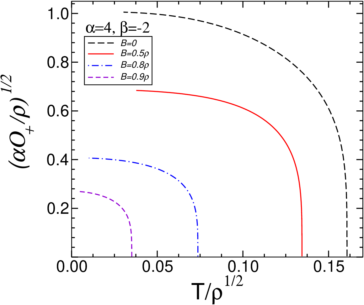
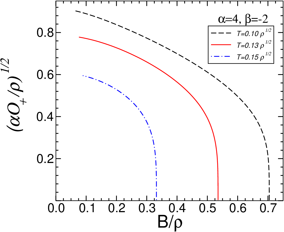
First, we report that this method is successful in constructing dyonic AdS black branes coupled to a neutral scalar field. From the holographic point of view, DDBBs are dual to field theories in which a neutral scalar operator acquires a non-vanishing expectation value below a critical temperature and below a critical magnetic field. In fact, in Fig. 7 we show the scalar condensate both as a function of the temperature for several values of constant magnetic field (left panel) and as a function of the magnetic field for several values of constant temperature (right panel) for $\alpha=4$ and $\beta=-2$ .

The phase diagram of DDBBs, i.e. the critical temperature as a function of the magnetic field, is shown in Fig. 8 for several values of the coupling $\alpha$ . The numerical results confirms our analytic expectation: $T_{c}=0$ when $B=B_{c}=\rho$ , i.e. the scalar operator does not condense at any finite temperature above the critical magnetic field $B_{c}$ . The critical value $B_{c}$ does not depend neither on the coupling constant $\alpha$ nor on the precise forms for $f(\phi)$ and $V(\phi)$ , when they behave as prescribed in Eq. (36).

Remarkably, Fig. 8 is qualitatively similar to Fig. 8 in Ref. [7], which describes the (qualitative) phase diagram for holographic superconductors immersed in a magnetic field.

The phase diagram for DDBBs shown in Fig. 8 is exact and confirms the schematic illustration depicted in Ref. [7].

Another interesting issue is the nature of the phase transition shown in the right panel of Fig. 7. At $B\sim B_{c}$ the scalar condensate has the typical behavior for second order phase transitions in the mean-field approximation,

O_{i}\sim(B-B_{c})^{1/2}\,.

(44)

This kind of phase transitions occurs in type-II superconductors. The same behavior is observed in real high- $T_{c}$ superconductors and it is correctly reproduced by holographic models [51]. However, in the case at hand, the new phase is not superconducting, as the neutral scalar operator preserves the $U(1)$ symmetry of the action (1). Nevertheless, also in this case we observe a sort of inverse-Meissner effect [48]: as the external magnetic field is increased, a second order phase transition occurs, and the condensate disappears. We stress that this effect occurs although the scalar condensate is homogeneous on the boundary.

V.2.2 Free energy and magnetic susceptibility of dyonic dilatonic black branes

As discussed above, a sufficiently strong magnetic field will destroy the new phase. The critical magnetic field can be also understood in terms of energetics. The difference in free energy between the normal and the dressed phase reads

\frac{B_{c}^{2}(T){\cal V}}{8\pi}=F_{\text{normal}}(T)-F_{\text{dressed}}(T)\,,

(45)

where ${\cal V}$ is the volume of $(x,y)$ plane and $F$ is the free energy. We wish to compare the free energy between different phases – with and without the scalar condensate – and in presence of a magnetic field. As for the normal phase, the free energy of a dyonic AdS-RN black hole (see for instance Ref. [7]) reads

\frac{F_{\text{RN}}}{{\cal V}}=\frac{F_{\text{normal}}}{{\cal V}}=-r_{h}^{3}+\frac{3(\rho^{2}+B^{2})}{4r_{h}}\,,

(46)

where we have set $L=1$ . In order to compute the free energy for DDBBs we start from the Euclidean action

S_{E}=-\int d^{4}x\sqrt{-G}{\cal L}\,,

(47)

where ${\cal L}$ is the Lagrangian written in (1) and computed for the numerical DDBB solution. Following Ref. [7] we write the Einstein tensor,

E_{xx}=\frac{r^{2}}{2}({\cal L}-R)+\frac{B^{2}f(\phi)}{2r^{2}}\,,

(48)

where $E_{\mu\nu}=R_{\mu\nu}-\frac{1}{2}G_{\mu\nu}R$ . Thus we obtain

{\cal L}=-E^{t}_{t}-E^{r}_{r}-\frac{B^{2}f(\phi)}{r^{4}}=-\frac{1}{r^{2}}\left[(rg)^{\prime}+(rge^{-\chi})^{\prime}e^{\chi}\right]-\frac{B^{2}f(\phi)}{r^{4}}\,,

(49)

where we have used the scalar curvature $R=-E^{a}_{a}$ computed for the dressed solution. Then the Euclidean action reads

S_{E}=\int d^{3}x\int_{r_{h}}^{\infty}dr\left(2rge^{-\chi/2}\right)^{\prime}+B^{2}\int d^{3}x\int_{r_{h}}^{\infty}dr\frac{f(\phi)e^{-\chi/2}}{r^{2}}\,.

(50)

The first radial integral in the equation above is a total derivative and it is straightforwardly performed. However, it diverges as $r\to\infty$ and must be regularized by suitable counterterms [7]. On the other hand, the contribution arising from the magnetic field is finite. Defining the regularized Euclidean action $\tilde{S}_{E}$ , the thermodynamical potential in the gran-canonical ensemble reads

\Omega=T\tilde{S}_{E}=\int d^{2}x\left(\frac{-\epsilon L^{2}}{2}+B^{2}\int_{r_{h}}^{\infty}dr\frac{f(\phi)e^{-\chi/2}}{r^{2}}\right)\,,

(51)

where $\epsilon$ is the energy density, we have defined the (compact) Euclidean time $\int dt=1/T$ , and we have used the boundary conditions (either ${\cal O}_{-}=0$ or ${\cal O}_{+}=0$ ) for the scalar field. Finally, the free energy of DDBBs in the canonical ensemble simply reads ( $L=1$ )

F_{\text{DD}}\equiv F_{\text{dressed}}=\Omega+\mu Q={\cal V}\left(-\frac{\epsilon}{2}+\mu\rho+B^{2}\int_{r_{h}}^{\infty}dr\frac{f(\phi)e^{-\chi/2}}{r^{2}}\right)\,.

(52)

In the particular case of AdS-RN black holes ( $f(\phi)\equiv 1$ and $\chi\equiv 0$ ) the integral above is trivial and $F_{\text{DD}}$ reduces to Eq. (46). In the left panel of Fig. 9 we compare $F_{\text{RN}}$ and $F_{\text{DD}}$ as functions of the temperature for selected values of the constant magnetic field. Free energies refers to solutions with same mass and same charge. Although not shown, for both solutions the specific heat $c=-T\partial_{T}F/{\cal V}$ is positive for any value of $B$ . AdS-RN black holes always have a larger free energy, for any value of $B$ and, roughly speaking, the magnetic field shifts the free energy of both solutions up. Therefore, when $T<T_{c}$ and $B<B_{c}$ , DDBBs are energetically favored. However, the magnetic field contributes to lower the difference $\Delta F=F_{RS}-F_{\text{DD}}$ . Such a difference grows as $T\to 0$ but, for fixed temperature, it decreases as the magnetic field increases. This is consistent with our analytical understanding, since we expect $\Delta F=0$ both when $T=T_{c}$ and when $B=B_{c}=\rho$ .

Finally, we can compute the magnetic susceptibility

\varXi=\left.{\frac{\partial^{2}F}{\partial B^{2}}}\right\rvert_{\rho,T}\,,

(53)

where the derivative is performed on solutions at constant temperature and constant charge density. Therefore in the numerical integration, we find the zeros of Eqs. (43), in order to compute the free energy as a function of the magnetic field at constant temperature and we obtain the magnetic susceptibility by performing the derivative in Eq. (53). Results are shown in the right panel of Fig. 9. The free energy and the magnetic field are normalized as $F\to F/\rho^{3/2}$ and as $B\to B/B_{c}$ , respectively. Hence, the magnetic susceptibility is normalized as $\varXi\to\varXi\rho^{3/2}/B_{c}^{2}$ .

The magnetic susceptibility $\varXi$ is order 1 and positive. This means that the boundary theory is strongly diamagnetic. This is analog to the AdS-RN case where $\varXi\sim 9/(8\pi T)>0$ for $B\ll M$ and $\rho\ll M$ [7].

V.3 Holographic properties of DDBBs

Let us now discuss some holographic properties of DDBBs. In particular we shall focus on the effects of the magnetic field on the electrical conductivity in the dual theory, such as the Hall effect and the presence of cyclotron resonances. The AdS/CFT correspondence provides a precise prescription for the computation of electrical conductivity of the dual field theory in terms of bulk electromagnetic perturbations. However, electromagnetic perturbations of a dyonic black hole are fairly involved. In fact, the minimal set of perturbations includes both the $x$ and $y$ components of the gauge potential $A_{x}(r)$ , $A_{y}(r)$ and the $tx$ and $ty$ components of the metric, $G_{tx}(r)$ and $G_{ty}(r)$ , which are coupled through the electric and magnetic field.

Perturbations of dyonic AdS-RN black holes have been studied in Refs. [52, 53]. Here we want to extend those calculations to the case of dilatonic background.

Let us consider perturbations with vanishing $3$ -momentum,

A_{\mu}=(A_{0},0,0,Bx)+(0,0,A_{x}(r),A_{y}(r))e^{-i\omega t}\,,

and similarly for the metric perturbations, $G_{tx}(r)e^{-i\omega t}$ and $G_{ty}(r)e^{-i\omega t}$ . Linearized Einstein and Maxwell equations provide a set of four coupled equations. Two of them are

	$\displaystyle A_{x}^{\prime\prime}+A_{x}^{\prime}\left(\frac{f^{\prime}(\phi)}{f(\phi)}\phi^{\prime}+\frac{g^{\prime}}{g}-\frac{\chi^{\prime}}{2}\right)+\omega^{2}\frac{e^{\chi}}{g^{2}}A_{x}$	$\displaystyle=$	$\displaystyle-e^{\chi}\left[\frac{iB\omega}{r^{2}g^{2}}G_{ty}+\frac{A_{0}^{\prime}}{g}\left(G_{tx}^{\prime}-\frac{2}{r}G_{tx}\right)\right],$		(54)
	$\displaystyle G_{tx}^{\prime}-\frac{2}{r}G_{tx}+f(\phi)A_{0}^{\prime}A_{x}$	$\displaystyle=$	$\displaystyle-\frac{iBf(\phi)}{r^{2}\omega}\left[A_{0}^{\prime}G_{ty}+ge^{-\chi}A_{y}^{\prime}\right]\,,$		(55)

and the other two can be obtained from those above by changing $x\leftrightarrow y$ and $B\leftrightarrow-B$ . Notice that terms proportional to $B$ couple perturbations along the $x$ direction to those along the $y$ direction. When $B=0$ equations above decouple and reduce to a single Schrödinger-like equation. In the case at hand, such a decoupling does not occur and we are left with a system of four coupled ODEs. Furthermore notice the presence of terms proportional to $B/\omega$ . When $B\neq 0$ these terms diverges in the $\omega\to 0$ limit, whereas they vanish if $B=0$ . Thus, as first noted in Ref. [52], the limits $B\to 0$ and $\omega\to 0$ do not commute.

We integrate the system of ODEs above numerically, starting from a series expansion close to the horizon, where we impose purely ingoing waves. The asymptotical behaviors read

	$\displaystyle A_{x}$	$\displaystyle\sim$	$\displaystyle a_{x}^{(0)}+a_{x}g_{h}^{\nu}\,,\qquad A_{y}\sim a_{y}^{(0)}+a_{y}g_{h}^{\nu}\,,$		(56)
	$\displaystyle G_{tx}$	$\displaystyle\sim$	$\displaystyle g_{x}^{(0)}+g_{x}g_{h}^{\nu+1}\,,\qquad G_{ty}\sim g_{y}^{(0)}+g_{y}g_{h}^{\nu+1}\,,$		(57)

with $g_{h}=g(r_{h})\sim(r-r_{h})$ and the requirement of purely ingoing waves at the horizon implies $\nu=-i\omega e^{\chi_{h}/2}/g^{\prime}(r_{h})$ . The constants $a_{x}$ , $a_{x}^{(0)}$ , $g_{x}$ , $g_{x}^{(0)}$ , $a_{y}$ , $a_{y}^{(0)}$ , $g_{y}$ and $g_{y}^{(0)}$ are related to each other by requiring that the expansions above are solutions of the equations of motion at first order.

V.3.1 Conductivity in the dual field theory

Before presenting the results of the numerical integration, we briefly review some analytical results obtained in Refs. [52, 53] for the electrical conductivity in theories dual to AdS-RN dyonic black hole. In that case, Eqs. (54)-(55) can be solved analytically in the hydrodynamical limit, i.e. when $\omega/T\ll\mu/T,B/T^{2}$ . In this limit the diagonal and off-diagonal components of the conductivity matrix ${\bf\sigma}$ can be computed via the AdS/CFT duality and they read [53]

\sigma_{xx}=\sigma_{Q}\frac{\omega(\omega+i\gamma+i\omega_{c}^{2}/\gamma)}{(\omega+i\gamma)^{2}-\omega_{c}^{2}}\,,\qquad\sigma_{xy}=-\frac{\rho}{B}\frac{-2i\gamma\omega+\gamma^{2}+\omega_{c}^{2}}{(\omega+i\gamma)^{2}-\omega_{c}^{2}}\ ,

with

\omega_{c}=\frac{B\rho}{\epsilon+{\cal P}}\,,\quad\gamma=\frac{\sigma_{Q}B^{2}}{\epsilon+{\cal P}}\,,\quad\sigma_{Q}=\frac{(sT)^{2}}{(\epsilon+{\cal P})^{2}}

(58)

and where ${\cal P}$ , $s$ and $\epsilon$ are the pressure, entropy density and the energy density respectively. Rotational invariance implies $\sigma_{xx}=\sigma_{yy}$ and $\sigma_{xy}=-\sigma_{yx}$ . The electrical conductivity has a pole at $\omega=\omega_{c}-i\gamma$ , corresponding to a damped cyclotron frequency. The real part $\omega_{c}$ does not depend on the temperature [53]. Furthermore, in the $\omega\to 0$ limit, the DC diagonal component $\sigma_{xx}$ vanishes, whereas the DC off-diagonal component gives the well-known Hall conductivity:

\sigma_{xx}=0\,,\qquad\sigma_{xy}=\frac{\rho}{B}\,.

(59)

Notice that $\sigma_{xy}\to\infty$ as $B\to 0$ . This is due to the non-commuting limits $\omega\to 0$ and $B\to 0$ .

It is important to study whether and how the scalar condensate affects these results. Unfortunately, in our model, the background solution is only known numerically and this prevents to derive explicit formulas. However we can still use the AdS/CFT prescription in order to relate the conductivity to the asymptotic behavior of the numerical solution. Following Ref. [53], the conductivity reads

\sigma_{\pm}=\sigma_{xy}\pm i\sigma_{xx}=\frac{{\cal B}_{x}\pm i{\cal B}_{y}}{{\cal E}_{x}\pm i{\cal E}_{y}}\,,

(60)

where

{\cal B}_{i}=-\lim_{r\to\infty}\epsilon_{ij}A_{j}^{\prime}\,,\qquad{\cal E}_{i}=\lim_{r\to\infty}\left[f(\phi)\left(i\omega A_{i}-\frac{B}{r^{2}}\epsilon_{ij}G_{tj}\right)\right]\,,

(61)

are the spatial components of $\delta F$ and $\delta\star F$ respectively ( $F=F_{0}+\delta F$ and $\star F=\star F_{0}+\delta\star F$ being its dual). The coefficients $A_{i}^{(0)}$ , $A_{i}^{(1)}$ and $G_{ti}^{(0)}$ are related to the asymptotic behavior of the electromagnetic and metric perturbations at infinity:

A_{i}\to A_{i}^{(0)}+\frac{A_{i}^{(1)}}{r}\,,\qquad G_{ti}\to G_{ti}^{(0)}r^{2}\,,\quad i=x,y

(62)

Thus, once perturbation equations are solved with suitable boundary conditions, Eq. (60) gives the AdS/CFT prescription for the conductivity in the dual theory.

V.3.2 Numerical results

In Fig. 10 we show the conductivities $\sigma_{xx}$ and $\sigma_{xy}$ as functions of the frequency both for the AdS-RN case ( $T=T_{c}$ ) and for the DDBB at $T<T_{c}$ . The numerical procedure previously discussed has been tested by reproducing numerical results in Ref. [53] for vanishing scalar field. A general result that can be inferred from our simulations is that, regardless of the scalar condensate, the DC conductivities are the same as those computed for AdS-RN black branes [53],

\sigma_{xx}(\omega\to 0)=0\,,\qquad\sigma_{xy}(\omega\to 0)=\frac{\rho}{B}\,,

(63)

at any $T\leq T_{c}$ . This result holds regardless of the precise form of $V(\phi)$ and $f(\phi)$ given by (36). While the first result ( $\sigma_{xx}=0$ ) simply arises from the Lorentz invariance, it is interesting that the Hall effect is not affected by the scalar condensate, for any value of $B$ .

However, as shown in Fig. 10, the AC behavior is more complex. Depending on the temperature and on the magnetic field, sharp peaks appear in the real part of $\sigma_{xx}$ and $\sigma_{xy}$ . These correspond to the (complex) cyclotron frequencies discussed in Ref. [53] for AdS-RN black branes. Our results confirm and extend that analysis to the case of DDBBs. Indeed the scalar condensate affects the cyclotron frequency. In Fig. 11 we show the location of the pole of $\sigma_{xx}$ as a function of the temperature for selected values of $B$ . Both the real and the imaginary part of the frequency strongly depend on the magnetic field (notice that the plot scale in Fig. 11 is logarithmic). The real part increases exponentially as the temperature is lowered, while the imaginary part, as a function of the temperature, has a less clear behavior, being monotonic at large values of $B$ and having a non-monotonic behavior at small values of $B$ .

VI Conclusion

In this paper we have presented a detailed study of the holographic properties of the 4D, charged, black brane solutions of broad classes of EMDG models both at finite and vanishing temperature and for different charge configurations (purely electric or magnetic, dyonic). Although our analysis is far from being exhaustive, it is likely that most of the qualitative relevant features concerning the holographic behavior of 4D charged dilatonic black branes in EMDG models have been captured by our investigation.

For what concerns the zero temperature limit, our results extend the results of Ref. [23, 19, 24] obtained in the case of a exponential coupling function $f$ to a broad class of EMDG models. In the $T\sim 0$ regime the AC conductivity has the universal scaling behavior, $\sigma_{AC}\sim\omega^{2}$ as a function of the frequency $\omega$ . For a generic form of the self-interaction potential $V(\phi)$ the quadratic behavior is generalized to a generic power-law form $\sigma_{AC}\sim\omega^{s}$ .

In view of the results of Ref. [23, 19, 24] one could have been lead to conclude that the power-law behavior of the conductivity is related to the Lifshitz form of the black brane metric in the near-extremal, near-horizon region. However, we have shown that this power-law behavior of $\sigma_{AC}$ is not spoiled if the Lifshitz form of the metric is (multiplicatively) deformed by powers of logarithms. This means that a power-law scaling behavior of $\sigma_{AC}$ is still consistent with a breaking of the non-relativistic scaling isometry of the Lifshitz background.

On the other hand the behavior of the DC conductivity in the zero temperature limit as a function of $T$ seems more involved. The quadratic scaling $\sigma_{DC}\sim T^{2}$ found in Ref. [24] for the case of a exponential coupling function $f$ , seems to be a quite general feature of EMDG models. This gives further support to the ‘charged plasma picture’ proposed in Ref. [24]. The electric conductivity is suppressed at small temperatures by strong repulsion. However, differently from the case of $\sigma_{AC}(\omega)$ discussed above, now the deformation of the Lifshitz form of the extremal black brane metric by logarithms, due to a power-law self-interaction potential, changes $\sigma_{DC}(T)$ (see Eq. (32)). This different behavior of $\sigma_{AC}(\omega)$ and $\sigma_{DC}(T)$ in the near-extremal case is somehow puzzling and a proper understanding of it could shed light on the physical nature of the dual field theory.

For what concerns black branes at finite temperature our results extend the results of Ref. [19], derived for the case of coupling functions $f\sim\cosh\alpha\phi$ and $f\sim 1+\alpha\phi^{2}$ , to a broad class of EMDG models. The non-monotonic behavior of $\sigma_{AC}(\omega)$ – characterized by a minimum at low frequencies and then by a ‘Drude peak’, at $\omega=0$ – and of $\sigma_{DC}(T)$ – characterized by the presence of a maximum, reminiscent of the Kondo effect – seem to be a rather generic feature of EMDG. In particular, we have shown that the emergence of these effects is not related to the presence of a phase transition RN/CDBB (as it is the case for the models of Ref. [19]) but shows up because of the nonmimimal coupling, whenever a sufficiently large scalar condensate is present.

Finally, our results concerning the holography of dyonic black branes at finite temperature confirm and extend to a broad class of EMDG the results of Ref. [24], derived for an exponential coupling function $f$ . Again, we have found that the main features observed in Ref. [24] (Hall effect, presence of synchrotron resonances) when a magnetic field is switched on, also apply to a the case of a coupling function $f$ that allows for a RN/CDBB phase transition. On the other hand, the switching on of a magnetic field does not shed much light on the nature of the microscopic degrees of freedom of the field theory dual to the models investigated in Ref. [19]. Naively, one could have expected this to be the case in view of the peculiar behavior of the AC and DC conductivities in absence of a magnetic field. Unfortunately, the effects of the magnetic field on the conductivities are so strong that any other effect becomes subleading and is completely washed out.

The overall picture emerging from our results about the holographic features of charged dilatonic black branes in EDGM can be described as an interpolation between some aspects reminiscent of electron motion in real metals at finite temperature and a charged plasma at zero temperature. It would be highly desirable to develop analytical methods to give further support to this picture.

Acknowledgements.

This work was partially supported by FCT - Portugal through projects PTDC/FIS/098025/2008, PTDC/FIS/098032/2008 and by the DyBHo–256667 ERC Starting Grant.

Appendix A Purely magnetic dilatonic black branes via the electromagnetic duality

In this appendix, we focus on the purely magnetic solutions, hereafter setting $Q=0$ . As discussed in the main text, in this case the AdS-RN black brane is stable and no magnetically charged dilatonic black branes exist. However, we can obtain purely magnetic solutions by applying the electromagnetic duality. In fact, a background solution characterized by coupling function, electric charge and magnetic charge $\{f(\phi),Q,B\}$ is related, via the electromagnetic duality, to the same background solution with $\{h=1/f,B,-Q\}$ . In particular the charged dilatonic black branes found in Ref. [19] are also valid magnetic solutions with $f\to 1/f$ and $B\to-Q$ .

For dyonic AdS-RN black branes, the duality acts on the electromagnetic tensor only

\frac{2\pi}{g^{2}}F\rightarrow\star F\equiv\frac{\sqrt{-g}}{4}\epsilon_{\mu\nu\rho\sigma}F^{\rho\sigma}dx^{\mu}\wedge dx^{\nu}\,.

(64)

Perturbation equations for $\delta F$ ( $F=F_{0}+\delta F$ ) are most conveniently written in terms of ${\cal B}_{a}$ and ${\cal E}_{a}$ , (cf. Eq. (61)) which are the spatial component of $\delta F$ and of $\delta\star F$ respectively. The electromagnetic duality acts as ${\cal E}\to{\cal B}$ and ${\cal B}\to-{\cal E}$ . It follows from Eq. (60) that the duality transforms the conductivities as

\sigma_{\pm}(Q,B)\rightarrow\frac{1}{\sigma_{\pm}(B,-Q)}\,.

(65)

Equation (65) has been recently extended to the case of SL(2,R) invariant theories with a dilaton and an axion [24]. Also in that case, starting from a purely electrical background, a transformation similar to (65) holds

\sigma_{\pm}(0,-Q)=\frac{1}{\sigma_{\pm}(Q,0)}\,,

(66)

which does not explicitly depend on the dilaton and axion fields. Although Eq. (66) has been derived for SL(2,R) invariant theories and the action (1) is not invariant under the full SL(2,R) transformation, nevertheless the same derivation should apply to our case as well. We shall explicitly confirm this statement below, by computing the conductivity in the purely magnetic case.

Electrical conductivity

Notice that, in the rest of this section, we keep referring to the coupling $f(\phi)$ for convenience, although the duality transformation acts on the action (1) by transforming $f\to h=1/f$ . The real non-minimal coupling for solutions obtained by the duality is $h(\phi)$ , not $f(\phi)$ . Furthermore, note that $h(\phi)\sim 1-\alpha\phi^{2}$ at $\phi\sim 0$ , whereas $f(\phi)\sim 1+\alpha\phi^{2}$ . The electromagnetic duality reverses the sign of $\alpha$ . This is why purely magnetic solutions exist in this case (cf. Eq. (39)).

For purely magnetic backgrounds, setting $A_{0}(r)\equiv 0$ , Eqs. (54)-(55) (and those obtained from them by $x\leftrightarrow y$ and $B\leftrightarrow-B$ ) decouple pairwise. Equations for $A_{x}$ and $G_{ty}$ read

	$\displaystyle A_{x}^{\prime\prime}+A_{x}^{\prime}\left(\frac{f^{\prime}(\phi)}{f(\phi)}\phi^{\prime}+\frac{g^{\prime}}{g}-\frac{\chi^{\prime}}{2}\right)+\omega^{2}\frac{e^{\chi}}{g^{2}}A_{x}+\frac{iB\omega}{r^{2}g^{2}}e^{\chi}G_{ty}$	$\displaystyle=$	$\displaystyle 0\,,$		(67)
	$\displaystyle G_{ty}^{\prime}-\frac{2}{r}G_{ty}-\frac{iBf(\phi)}{r^{2}\omega}ge^{-\chi}A_{x}^{\prime}$	$\displaystyle=$	$\displaystyle 0\,,$		(68)

and those for $A_{y}$ and $G_{tx}$ can be again obtained by $x\leftrightarrow y$ and $B\leftrightarrow-B$ . The two equations above can be written in terms of a single Schrödinger-like equation for $A_{x}^{\prime}(r)$ , i.e. they are third order in $A_{x}(r)$ . In fact, we define

A_{x}^{\prime}(r)=\frac{e^{\chi/2}}{g(r)\sqrt{f(\phi)}}Y(r)\,,

(69)

and the equation for $Y(r)$ reads

Y^{\prime\prime}(r)+\left(\frac{g^{\prime}}{g}-\frac{\chi^{\prime}}{2}\right)Y^{\prime}(r)+\frac{e^{\chi}}{g^{2}}\left[\omega^{2}-V_{s}\textyen(r)\right]Y(r)=0\,,

(70)

or, equivalently,

Y^{\prime\prime}(z)+\left[\omega^{2}-V_{s}\textyen(z)\right]Y(z)=0\,,

(71)

where $z$ is the tortoise coordinate defined by $dr/dz=e^{\chi(r)/2}/g(r)$ and the explicit form of the potential reads

V_{s}\textyen(z)=ge^{-\chi}\left\{\frac{B^{2}f(\phi)}{r^{4}}-\frac{g}{2}\frac{f^{\prime}(\phi)}{f(\phi)}\left[\phi^{\prime\prime}+\left(\frac{f^{\prime\prime}(\phi)}{f^{\prime}(\phi)}-\frac{3}{2}\frac{f^{\prime}(\phi)}{f(\phi)}\right)\phi^{\prime 2}+\left(\frac{g^{\prime}}{g}-\frac{\chi^{\prime}}{2}\right)\phi^{\prime}\right]\right\}\,.

(72)

Interestingly, in the equation above the magnetic field dependence is $B^{2}$ and the contribution $\propto 1/\omega$ of Eq. (68) cancels out, i.e. in the purely magnetic case the limits $B\to 0$ and $\omega\to 0$ commute.

For a magnetic AdS-RN black brane ( $\chi\equiv 0$ and $\phi\equiv 0$ ) the potential above simply reduces to

V_{RS}=g_{RS}(r)\frac{B^{2}}{r^{4}}\,,

(73)

and it is positive defined. Moreover $V_{RS}=0$ at the horizon and at infinity. From general quantum mechanics theorems it follows that such a Schrödinger potential does not admit bound states, i.e. the magnetic AdS-RN black brane is stable. The potential for purely magnetic dilatonic solutions (obtained via the electromagnetic duality) is shown in Fig. 12. Also in this case the potential is positive defined and the background solution is stable.

Numerical results

As non-trivial test of our numerical method, we have computed the conductivity $\sigma_{+}(\omega)$ in a purely electrical background and compared it to the inverse of the conductivity in a purely magnetic background $\sigma_{+}^{-1}(\omega)$ with $f(\phi)\to 1/f(\phi)$ . A representative example is shown in Fig. 13. The two functions coincide, confirming analytical expectations (cf. Eq. (66) and Ref. [24]).

Notice that, although the electromagnetic duality straightforwardly relates the conductivities $\sigma_{\pm}$ in an electrical and in a magnetic background, nevertheless the transformation is non-trivial and it connects the conductivities computed in two different theories (the couplings in the action are different). Furthermore, not only $\sigma_{\pm}$ are complex quantities, but, above all, the physically interesting quantities are the frequencies $\sigma_{xx}$ and $\sigma_{xy}$ . Namely, the explicit transformations for these quantities read

\sigma_{xy}^{M}=\frac{\sigma_{xy}^{E}}{\left(\sigma_{xx}^{E}\right)^{2}+\left(\sigma_{xy}^{E}\right)^{2}}\,,\quad\sigma_{xx}^{M}=-\frac{\sigma_{xx}^{E}}{\left(\sigma_{xx}^{E}\right)^{2}+\left(\sigma_{xy}^{E}\right)^{2}}\,,\quad\text{Re}[\sigma_{M}]=\frac{\text{Re}[\sigma_{E}]}{\text{Abs}[\sigma_{E}]^{2}}\,,\quad\text{Im}[\sigma_{M}]=-\frac{\text{Im}[\sigma_{E}]}{\text{Abs}[\sigma_{E}]^{2}}\,,

(74)

where $\sigma^{M}$ and $\sigma^{E}$ are the electrical conductivities in the magnetic and electrical case, respectively and all the quantities are complex. Therefore the explicit dependence of, say, $\text{Re}\left[\sigma^{M}_{xx}\right]$ can be non-trivial. In the left panel of Fig. 14 we show the AC conductivity $\sigma_{xx}(\omega)$ for a purely magnetic background solution. From our numerical simulations we can infer the general behavior

\sigma_{xy}(\omega)\equiv 0\,,\qquad\sigma_{xx}(\omega\sim 0)=0\,,

(75)

that is, for any temperature, the off-diagonal component of the conductivity vanishes at any frequency. However, as shown in the left panel of Fig. 14, the AC diagonal component has a maximum whose location and height depend on the temperature. These peaks in the conductivity may signal the excitation of some bound state in the dual field theory. Thus $\sigma^{M}$ , although related to $\sigma^{E}$ by the electromagnetic duality, can show some non-trivial features.

The Zero temperature limit of purely magnetic DDBs

For the sake of completeness, let us conclude this section by briefly discussing extremal magnetic DBBs. Purely magnetic background solutions can be again obtained from purely electrical extremal backgrounds via the electromagnetic duality. Extremal electrical solutions have been discussed in detail in Ref. [19]. They are most conveniently studied using the ansatz (17). Using this ansatz perturbation equations around dyonic background solutions read

	$\displaystyle A_{x}^{\prime\prime}+A_{x}^{\prime}\left(\frac{f^{\prime}(\phi)}{f(\phi)}\phi^{\prime}+\frac{\lambda^{\prime}}{\lambda}\right)+\frac{\omega^{2}}{\lambda^{2}}A_{x}+\frac{iB\omega}{H^{2}\lambda^{2}}G_{ty}+\frac{A_{0}^{\prime}}{\lambda}\left(G_{tx}^{\prime}-\frac{2H^{\prime}}{H}G_{tx}\right)$	$\displaystyle=$	$\displaystyle 0\,,$		(76)
	$\displaystyle G_{tx}^{\prime}-\frac{2H^{\prime}}{H}G_{tx}+f(\phi)A_{0}^{\prime}A_{x}+\frac{iBf(\phi)}{H^{2}\omega}\left[A_{0}^{\prime}G_{ty}+\lambda A_{y}^{\prime}\right]$	$\displaystyle=$	$\displaystyle 0\,,$		(77)

plus those obtained via $x\leftrightarrow y$ and $B\leftrightarrow-B$ . As previously discussed, in a purely magnetic background ( $A_{0}(r)\equiv 0$ ) perturbation equations decouple and can be written as a Schrödinger equation. Following the derivation described by Eqs. (69)-(72), we obtain a Schrödinger-like equation, $Y^{\prime\prime}(z)+\left[\omega^{2}-V_{s}\textyen(z)\right]Y(z)=0$ , where the potential reads

V_{s}\textyen(z)=\lambda\left\{\frac{B^{2}f(\phi)}{H^{4}}-\frac{\lambda}{2}\frac{f^{\prime}(\phi)}{f(\phi)}\left[\phi^{\prime\prime}+\left(\frac{f^{\prime\prime}(\phi)}{f^{\prime}(\phi)}-\frac{3}{2}\frac{f^{\prime}(\phi)}{f(\phi)}\right)\phi^{\prime 2}+\frac{g^{\prime}}{g}\phi^{\prime}\right]\right\}\,.

(78)

where $dr/dz=1/\lambda$ and $Y(z)=\sqrt{f(\phi)}\lambda A^{\prime}_{x}\textyen$ . The conductivity as a function of the frequency at $T=0$ is shown in the right panel of Fig. 14. Also in this case the real part of $\sigma_{xx}(\omega)$ shows a peak at intermediate frequencies.

References

[1] J. M. Maldacena, Adv. Theor. Math. Phys. 2, 231 (1998), eprint hep-th/9711200.
[2] S. Sachdev and M. Mueller, J. Phys.: Condens. Matter 21, 164216 (2009), eprint 0810.3005.
[3] C. P. Herzog, J. Phys. A42, 343001 (2009), eprint 0904.1975.
[4] S. A. Hartnoll, Class. Quant. Grav. 26, 224002 (2009), eprint 0903.3246.
[5] J. McGreevy, Adv. High Energy Phys. 2010, 723105 (2010), eprint 0909.0518.
[6] S. S. Gubser and S. S. Pufu, JHEP 11, 033 (2008), eprint 0805.2960.
[7] S. A. Hartnoll, C. P. Herzog, and G. T. Horowitz, JHEP 12, 015 (2008a), eprint 0810.1563.
[8] S. A. Hartnoll, C. P. Herzog, and G. T. Horowitz, Phys. Rev. Lett. 101, 031601 (2008b), eprint 0803.3295.
[9] S.-J. Rey, Prog. Theor. Phys. Suppl. 177, 128 (2009), eprint 0911.5295.
[10] S.-S. Lee, Phys. Rev. D79, 086006 (2009), eprint 0809.3402.
[11] H. Liu, J. McGreevy, and D. Vegh (2009), eprint 0903.2477.
[12] M. Cubrovic, J. Zaanen, and K. Schalm, Science 325, 439 (2009), eprint 0904.1993.
[13] T. Faulkner, H. Liu, J. McGreevy, and D. Vegh (2009), eprint 0907.2694.
[14] B. McInnes, Nucl. Phys. B832, 323 (2010), eprint 0910.4456.
[15] T. Faulkner, G. T. Horowitz, and M. M. Roberts (2010), eprint 1008.1581.
[16] A. R. Lugo, E. F. Moreno, and F. A. Schaposnik, JHEP 03, 013 (2010), eprint 1001.3378.
[17] E. D’Hoker and P. Kraus, JHEP 05, 083 (2010), eprint 1003.1302.
[18] M. J. Duff and J. T. Liu, Nucl. Phys. B554, 237 (1999), eprint hep-th/9901149.
[19] M. Cadoni, G. D’Appollonio, and P. Pani, JHEP 03, 100 (2010), eprint 0912.3520.
[20] C. Charmousis, B. Gouteraux, B. S. Kim, E. Kiritsis, and R. Meyer, JHEP 11, 151 (2010), eprint 1005.4690.
[21] D. D. Doneva, S. S. Yazadjiev, K. D. Kokkotas, I. Z. Stefanov, and M. D. Todorov, Phys. Rev. D81, 104030 (2010), eprint 1001.3569.
[22] S. S. Gubser and F. D. Rocha, Phys.Rev. D81, 046001 (2010), eprint 0911.2898.
[23] K. Goldstein, S. Kachru, S. Prakash, and S. P. Trivedi, JHEP 08, 078 (2010a), eprint 0911.3586.
[24] K. Goldstein et al., JHEP 10, 027 (2010b), eprint 1007.2490.
[25] C.-M. Chen and D.-W. Pang, JHEP 06, 093 (2010), eprint 1003.5064.
[26] B.-H. Lee, S. Nam, D.-W. Pang, and C. Park (2010a), eprint 1006.0779.
[27] B.-H. Lee, D.-W. Pang, and C. Park, JHEP 07, 057 (2010b), eprint 1006.1719.
[28] Y. Liu and Y.-W. Sun, JHEP 07, 099 (2010), eprint 1006.2726.
[29] B.-H. Lee, D.-W. Pang, and C. Park, JHEP 11, 120 (2010c), eprint 1009.3966.
[30] G. Bertoldi, B. A. Burrington, A. W. Peet, and I. G. Zadeh (2011), eprint 1101.1980.
[31] G. Bertoldi, B. A. Burrington, and A. W. Peet, Phys. Rev. D82, 106013 (2010), eprint 1007.1464.
[32] E. Perlmutter, JHEP 02, 013 (2011), eprint 1006.2124.
[33] G. W. Gibbons and K.-i. Maeda, Nucl. Phys. B298, 741 (1988).
[34] D. Garfinkle, G. T. Horowitz, and A. Strominger, Phys. Rev. D43, 3140 (1991).
[35] M. Cadoni and S. Mignemi, Phys. Rev. D 48, 5536 (1993), eprint 9305107.
[36] S. Monni and M. Cadoni, Nucl. Phys. B466, 101 (1996), eprint hep-th/9511067.
[37] C. Charmousis, B. Gouteraux, and J. Soda, Phys. Rev. D80, 024028 (2009), eprint 0905.3337.
[38] S. Mignemi (2009), eprint 0907.0422.
[39] G. T. Horowitz and J. Polchinski (2006), eprint gr-qc/0602037.
[40] P. Breitenlohner and D. Z. Freedman, Phys. Lett. B115, 197 (1982).
[41] I. R. Klebanov and E. Witten, Nucl. Phys. B556, 89 (1999), eprint hep-th/9905104.
[42] T. Hertog and G. T. Horowitz, JHEP 07, 073 (2004), eprint hep-th/0406134.
[43] F. Aprile and J. G. Russo, Phys.Rev. D81, 026009 (2010), eprint 0912.0480.
[44] S. A. Hartnoll, J. Polchinski, E. Silverstein, and D. Tong, JHEP 04, 120 (2010), eprint 0912.1061.
[45] G. T. Horowitz and M. M. Roberts, JHEP 11, 015 (2009), eprint 0908.3677.
[46] N. M. R. Peres, Rev. Mod. Phys. 82, 2673 (2010), eprint 1007.2849.
[47] S. Sachdev, J.Stat.Mech. 1011, P11022 (2010), eprint 1010.0682.
[48] T. Albash and C. V. Johnson, JHEP 09, 121 (2008), eprint 0804.3466.
[49] M. Montull, A. Pomarol, and P. J. Silva, Phys. Rev. Lett. 103, 091601 (2009), eprint 0906.2396.
[50] P. P. Fiziev and D. R. Staicova (2010), eprint 1005.5375.
[51] G. T. Horowitz (2010), eprint 1002.1722.
[52] S. A. Hartnoll and P. Kovtun, Phys. Rev. D76, 066001 (2007), eprint 0704.1160.
[53] S. A. Hartnoll and C. P. Herzog, Phys. Rev. D76, 106012 (2007), eprint 0706.3228.