Recoiled star clusters in the Milky Way halo: N-body simulations and a candidate search through SDSS
Abstract
During the formation of the Milky Way, central black holes (BHs) may have been ejected from their small host galaxies as a result of asymmetric gravitational wave emission. We previously showed that many of these BHs are surrounded by a compact cluster of stars that remained bound to the BH during the ejection process. In this paper, we perform long term -body simulations of these star clusters to determine the distribution of stars in these clusters today. These numerical simulations, reconciled with our Fokker-Planck simulations, show that stellar density profile follows a power-law with slope , and show that large angle scattering and tidal disruptions remove of the stars by yr. We then analyze the photometric and spectroscopic properties of recoiled clusters accounting for the small number of stars in the clusters. We use our results to perform a systematic search for candidates in the Sloan Digital Sky Survey. We find no spectroscopic candidates, in agreement with our expectations from the completeness of the survey. Using generic photometric models of present day clusters we identify recoiling cluster candidates. Follow-up spectroscopy would be able to determine the nature of these candidates.
Keywords:
galaxies:kinematics and dynamics–galaxies:nuclei–black hole physics–gravitational waves–star clusters1 Introduction
1.1 Motivation
In the standard cosmological context of hierarchical galaxy formation, the first galaxies to form were small () and grew through subsequent accretion and mergers (Loeb, 2010). If central black holes (BHs) were common in the earliest epochs of galaxy formation, then for most major mergers, the two BHs would also eventually merge. If there were any asymmetry in the inspiral and coalescence of two BHs, whether due to a difference in mass, or the alignment of the BHs’ spin vectors, then there would inevitably be a net linear momentum kick to the merger remnant (Peres, 1962; Bekenstein, 1973; Fitchett, 1983). This kick, which is typically hundreds of for mergers with comparable masses (Baker et al., 2006; Campanelli et al., 2007b; Campanelli et al., 2007a; Tichy & Marronetti, 2007), is independent of the total mass of the BHs. Thus, such kicks have the greatest dynamical effect in the smallest galaxies (Madau & Quataert, 2004; Libeskind et al., 2006; Micic et al., 2006; Volonteri, 2007; Schnittman, 2007; Blecha & Loeb, 2008). Indeed, a major merger in the first galaxies would inevitably lead to the ejection of the BH. Interestingly, the typical kick velocity is smaller than the escape velocity of the Milky Way halo, and so, although the first galaxies to merge would have lost their BHs, many of these ’rogue’ BHs should remain in the Milky Way halo today (Madau & Quataert, 2004; Volonteri & Perna, 2005; Libeskind et al., 2006; Micic et al., 2008; O’Leary & Loeb, 2009).
Before coalescence, the BH-BH binary may be surrounded by both a disk of dense gas and a dense cusp of stars. For bound matter with orbital velocities larger than the kick velocity, the gravitational wave kick perturbs the orbit of the material, but does not unbind it from the recoiled BH even if the BH is ejected from the galaxy (Loeb, 2007). For gas disks, viscosity eventually causes the BH to accrete the surrounding gas on order of a few Myr, leaving the BH as a short lived quasar (Loeb, 2007; Blecha & Loeb, 2008; Guedes et al., 2010; Sijacki et al., 2010; Blecha et al., 2011). After depleting all bound gas, the BHs will only be visible if they pass through dense gas in the galaxy and reaccrete material (Islam et al., 2004b; Islam et al., 2004a; Volonteri & Perna, 2005; Mii & Totani, 2005; Bertone et al., 2005; Blecha & Loeb, 2008). Stars, on the other hand, are effectively collisionless, and will remain bound as a long lived system (Gualandris & Merritt, 2008; Komossa & Merritt, 2008; O’Leary & Loeb, 2009; Merritt et al., 2009), and may actually be tidally disrupted by the BH after ejection (Komossa & Merritt, 2008) or produce winds providing a new source of gas accretion to the black hole (O’Leary & Loeb, 2009).
In O’Leary & Loeb (2009; hereafter as Paper I), we used merger tree histories of the Milky Way galaxy to calculate the number and mass distribution of these recoiled BHs. We assumed that after a major merger, with galaxy mass ratio greater than 1:10, the black holes merged immediately. We found that BHs with should be in the halo today, surrounded by compact star clusters that are of their BH’s mass (see Merritt et al., 2009, for a similar discussion applied to the nearby Virgo Cluster). These clusters are expected to roughly follow the dark matter distribution of the halo, since they have kick velocities typically less than the velocity dispersion of the galaxy. At their typical distances dynamical friction is not important over a Hubble time. The most massive star clusters have a much higher internal velocity dispersion than globular clusters because they are gravitationally bound by the BH at their center. Finding these clusters in the Milky Way halo will allow us to peer back in time and look at some of the first BHs to form. In this paper we re-investigate the long term evolution of recoiled star clusters using full -body simulations, with a one-to-one correspondence between stars and -body particles. We also extend the Fokker-Planck simulations from Paper I to include large-angle scattering between stars in order to reconcile these new simulations with our results from Paper I, and extend the reach of our simulations to larger BHs. We use the results of these simulations to generate the photometric properties of recoiled clusters. Because these clusters have so few stars, stochastic variation dominates over the dispersion of the cluster colors. Instead of using averaged stellar evolution tracks of old star systems, we use a Monte-Carlo approach to generate individual star cluster colors and sizes to identify the typical properties of these systems and compare them to the properties of stars and galaxies in the the Sloan Digital Sky Survey11 1 http://www.sdss.org/dr7/ Data Release 7 (Abazajian et al., 2009, hereafter SDSS DR7).
Our paper is organized as follows. In § 1.2, we describe recoiled clusters and briefly summarize the main results from Paper I. In § 2, we use -body simulations to follow the long term dynamical evolution of recoiled star clusters. We then extend our previous Fokker-Planck analysis in § 3 to include the ejection of stars from large angle scattering. In § 4, we develop a series of simple photometric models that we use to search for recoiled clusters in § 5. In § 6, we search the spectroscopic database of SDSS for candidate clusters. Finally in § 8, we summarize our paper and describe the main conclusions.
1.2 Stellar Cusps and Recoiled Black Holes
For a relaxed stellar system around a central massive BH, Bahcall & Wolf (1976) found that the stellar density follows a power-law profile within the radius of influence of the BH, , where is the BH mass, and is the stellar velocity dispersion. Out to the radius where the total mass in stars around the BH is twice the mass of the BH the density profile is
| (1) |
where for a cluster of single mass stars of mass . If the binary black hole merges on a timescale comparable to the relaxation time, then the Bahcall & Wolf (1976) cusp will be regenerated as the binary inspirals. However, if the binary merges on a shorter timescale than the relaxation time (e.g., through its interaction with gas ), then the stellar density profile is expected to be much shallower with and with fewer stars within (Merritt & Szell, 2006; Merritt et al., 2007). For the BH masses we consider here, the relaxation timescale is much less than the age of the universe,
| (2) |
The kick on the BH remnant occurs over a timescale much shorter than the orbital time of the stars. Therefore, in the frame of the BH, the stars all instantaneously receive a kick, . To first order, stars with a total energy , will remain bound to the BH as it is ejected from the galaxy. For the Keplerian potential of the BH, this approximately corresponds to all stars with . From equation (1), this corresponds to a number of stars
| (3) |
where we set , and used the relation to determine (Tremaine et al., 2002).
The star cluster will begin to expand away from the BH immediately after it is ejected from the galaxy. In Paper I, we followed the long term evolution of the star cluster by numerically integrating the time dependent, one-dimensional Fokker-Planck equation for stars around a central BH. We found that the density cusp of stars around the BH quickly expands to the point that the relaxation timescale of the system is approximately its age . In our simulations, the total mass in stars was roughly constant. However, our calculations could not consistently account for either strong encounters or resonant interactions between stars. In both cases, we would expect a larger fraction of stars to be ejected or destroyed.
We estimated the number of recoiled BHs in the Milky Way Halo using an ensemble of merger tree histories of the Milky Way, convolved with the probability distribution of kick velocities (Schnittman & Buonanno, 2007). We found that a typical Milky Way like galaxy contains as many as recoiled BHs with , with a mass spectrum . Because the kick velocity distribution peaks at low velocities, , the majority of recoiled clusters had the minimal kick velocity needed to escape from the host galaxy. In Paper I, we estimated this to be immediately after the galaxy merger. Overall, these results were consistent with previous studies that looked at a population of BHs in the Milky Way halo, whether from gravitational wave recoil, through three body encounters, or as the remnants of the seed population of black holes (Madau & Quataert, 2004; Volonteri & Perna, 2005; Libeskind et al., 2006; Micic et al., 2008)
2 -Body Simulations
Small star clusters around recoiled BHs present an interesting dynamical system that can be modeled directly in -body simulations, as well as through approximate methods such as solving the Fokker-Planck equation. Because some star clusters have only a few thousand stars, it is possible to simulate the star clusters with a one to one correspondence between stars and -body particles. In this section, we simulate the star clusters directly, and compare the results to our previous Fokker-Planck simulations from Paper I.
2.1 Method
We use the publicly available -body code BHint22 2 Available at http://www.astro.uni-bonn.de/english/downloads.php (Löckmann & Baumgardt, 2008) to simulate the long term evolution of star clusters around recoiled BHs. BHint was developed to precisely integrate the equations of motion of stellar systems around massive BHs, where the BH dominates the motion of the stars.
The initial conditions for the recoiled BH and star cluster are set up by first generating Bahcall & Wolf (1976) stellar density cusps around a BH, following equation (1), with , such that the total mass of stars within is twice that of the black hole. The stars’ velocities are initially selected from a Gaussian distribution with , where , which is an excellent approximation to the velocity distribution of stars in a power-law density cusp. We use two model mass functions for the stars. In Model I we use equal-mass stars with . In Model II, we use a more realistic mass function to model a population of old stars. Although massive stars likely play an important role in the evolution of clusters, they are short lived compared to the cluster lifetime. Stars with mass , evolve to form neutron stars or white dwarfs, which are comparable in mass to long lived main sequence stars, and so should not significantly alter the dynamics of the system except to increase the mass-to-light ratio33 3 The total amount of mass lost is , and will accordingly only perturb the orbits of the stars.. More massive stars form black holes, with mass , which may dramatically alter the dynamics of the system. These black holes may even segregate before the binary merges (Morris, 1993; Merritt, 2009). If the black holes dominate the dynamical evolution of the system, such systems may not have any luminous stars to observe. However the fraction of black holes in the region immediately after reforming the cusp is highly uncertain, and so we take the extreme opposite approach and ignore the black hole population. Assuming that there are very few black holes, which may be the case in a subset of the recoiled clusters, we use a relatively flat mass function for low mass stars () with . The mass of each star is generated randomly following this distribution until the total mass of the cusp reaches . We use such a shallow power law because of the break in the initial mass function at (Kroupa, 2001).
After generating the cusps for Models 1 & 2, we then kick each star with a velocity , and remove all stars that are unbound to the BH. Approximately of stars remain bound to the black hole. With these assumptions we do not account for stars that are originally unbound to the black hole. However, unbound stars do not contribute significantly in numbers deep within a full cusp.
We run the simulations for yr, the approximate age of the clusters. Stars are removed from the simulation if they are ejected from the cluster, , if they reach a separation pc, or if they are tidally disrupted by the central BH44 4 We have also simulated clusters with a much smaller tidal disruption radius in order to look at how this may affect the inner density profile., . For each star that is tidally disrupted, we add its total mass to the BH. All of our -body simulations follow clusters with and . For all of the reported simulations we set the time step criterion and the stars orbits were evaluated at minimum 80 times per orbit. We have checked the simulations with more precise parameters ( and 160 evaluations per orbit) and found similar results. We simulate 40 different cluster realizations for each Model and average over all the runs. A typical simulation takes up to one month on a single core of the Odyssey Cluster at Harvard University.
2.2 -Body Results
2.2.1 Cluster Evolution and Expansion
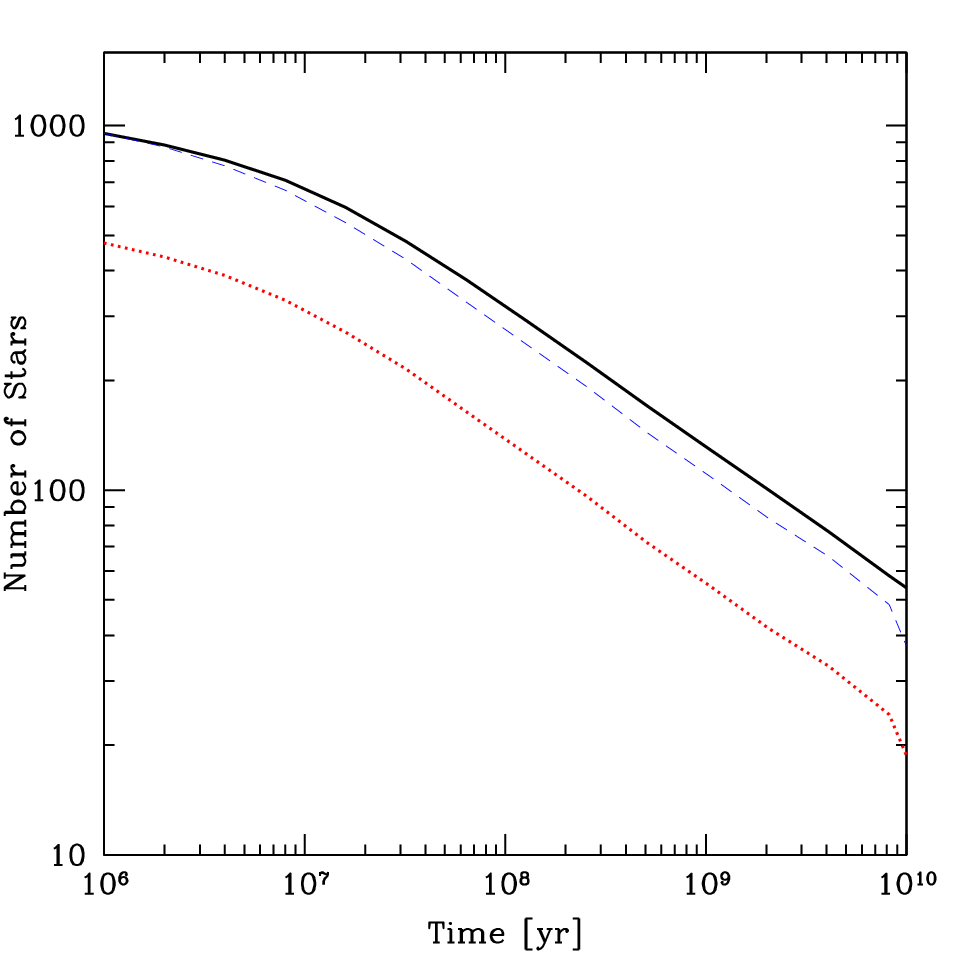
Immediately after the recoil, the BH is ejected with of bound stars, in rough agreement with our initial estimates. In Figure 1, we plot the average number of stars bound to the recoiled BH as a function of time for Models I & II. After a relaxation timescale, , the star cluster begins to expand and lose stars as a power-law with . Approximately of the stars are ejected from the cluster and another of the stars are tidally disrupted by the BH (see § 2.2.2). After both Models begin to evolve, the ratio of the total mass of stars in each Model remains constant in time.
In our simulations there are effectively only 3 parameters that determine the cluster evolution: the BH mass, , the average stellar mass, , and the kick velocity . All other scales in the simulation were determined through the relation55 5 The tidal disruption radius depends on the mass ratio of the BH and star, however we found that the final number of stars in our simulations was insensitive to the chosen tidal disruption radius.. Since the required kick velocity to eject the BH scales with , and the total number of stars in the cluster scales with the BH mass (), we can rescale the results of our simulations to find the number of stars in a recoiled cluster as a function of time () at yr,
| (4) |
for a fixed , and where we have normalized the scaling relation to match our -body simulations. The more massive the BH is, the fewer number of relaxation timescales the cluster will undergo over a fixed duration in time. Equations (3) & (4) are equivalent at when . For BHs with masses above this value, the total number of stars in the cluster matches the initial number of stars at recoil. This has important implications for recoiled clusters near elliptical galaxies and galaxy clusters (Merritt et al., 2009, see). For star clusters with , such as those we expect around the Milky Way, the cluster will lose many of its initial stars and have evolved from its original state. From equation (4), and the power-law nature of Figure 1, for a fixed average stellar mass, we expect the final number of stars in the cluster will not be significantly larger even if the cluster had more stars initially; it would instead begin to decay earlier, following the same overall functional form .
In Figure 2, we plot the normalized velocity spectrum of stars ejected from Models I and II as a function of time, looking at the first, second, and last third of stars ejected from the cluster. The typical velocity of an ejected star is usually a fraction of the velocity dispersion of the cluster, which decreases with time as the cluster expands. The total velocity distribution of all the stars ejected from cluster appears almost log-normal, independent of the mass function of stars, with a peak at , and full-width half maximum an order of magnitude above the peak value. On average, nearly twice as many stars were ejected from Model II ( per cluster) compared to Model I ( per cluster). However, the total mass of stars ejected is comparable. From the velocity spectrum, we see that the slow diffusion of stars to higher energies can not be the cause of the cluster evaporation. If this were the case, the ejection spectrum would peak near zero velocity, as most stars become unbound just as they approach the escape velocity of the cluster. In fact, the peak velocity of the ejected stars is near , a reflection of large angle scattering (Henon, 1969; Lin & Tremaine, 1980). Indeed, this is confirmed by the pericenter distance of the stars before they are ejected, which is always much smaller than the half-mass radius of the cluster and the boundary of our simulations, pc. Nearly all of the ejected stars will remain bound to the Milky Way halo (). Only a few of the earliest stars ejected from the cluster have large enough velocities to constitute a hypervelocity star (Brown et al., 2005; Yu & Tremaine, 2003). This, of course, is a small fraction of the number of hypervelocity stars that are expected to be produced during the inspiral of the BH binary (Yu & Tremaine, 2003).


After approximately one relaxation timescale, the cluster begins to expand as it is heated by the innermost star in the cluster as well as by tidal disruptions. We find in our -body simulations that radii that enclose a fixed number of stars scale as a power-law . The same relation is observed in our Fokker-Planck simulations (see § 3.1), in previous simulations of black holes in star clusters (Amaro-Seoane et al., 2004, see, e.g.,), as well as in previous work exploring the expansion of a cluster without a black hole post core-collapse (see, e.g., Hénon, 1961; Goodman, 1984, and citing articles.). The power-law index can be obtained by looking at the flow of energy through the cluster, so long as the energy is generated in a sufficiently small volume. Following, Gieles et al. (2011) (Hénon, 1961; Hénon, 1965, see also,), we can analyse the flow of energy
| (5) |
at a radius that encloses a fixed number, , of stars. Here, , is independent of , and . Under the assumption that the rate of stars being ejected from the cluster is small (), we can solve for as a function of . For a cluster in the Keplerian potential of a black hole, . Solving Eq. 5, then yields . A similar relation can be found for the expansion of a cluster without a black hole post core-collapse (see, e.g., Hénon, 1961; Hénon, 1965; Goodman, 1984, and citing articles.), which yields the same proportionality, however for a different reason (). As the ejection of stars from the cluster becomes important, however, we expect the cluster evolution to deviate from .
2.2.2 Tidal Disruption of Stars & Resonant Relaxation
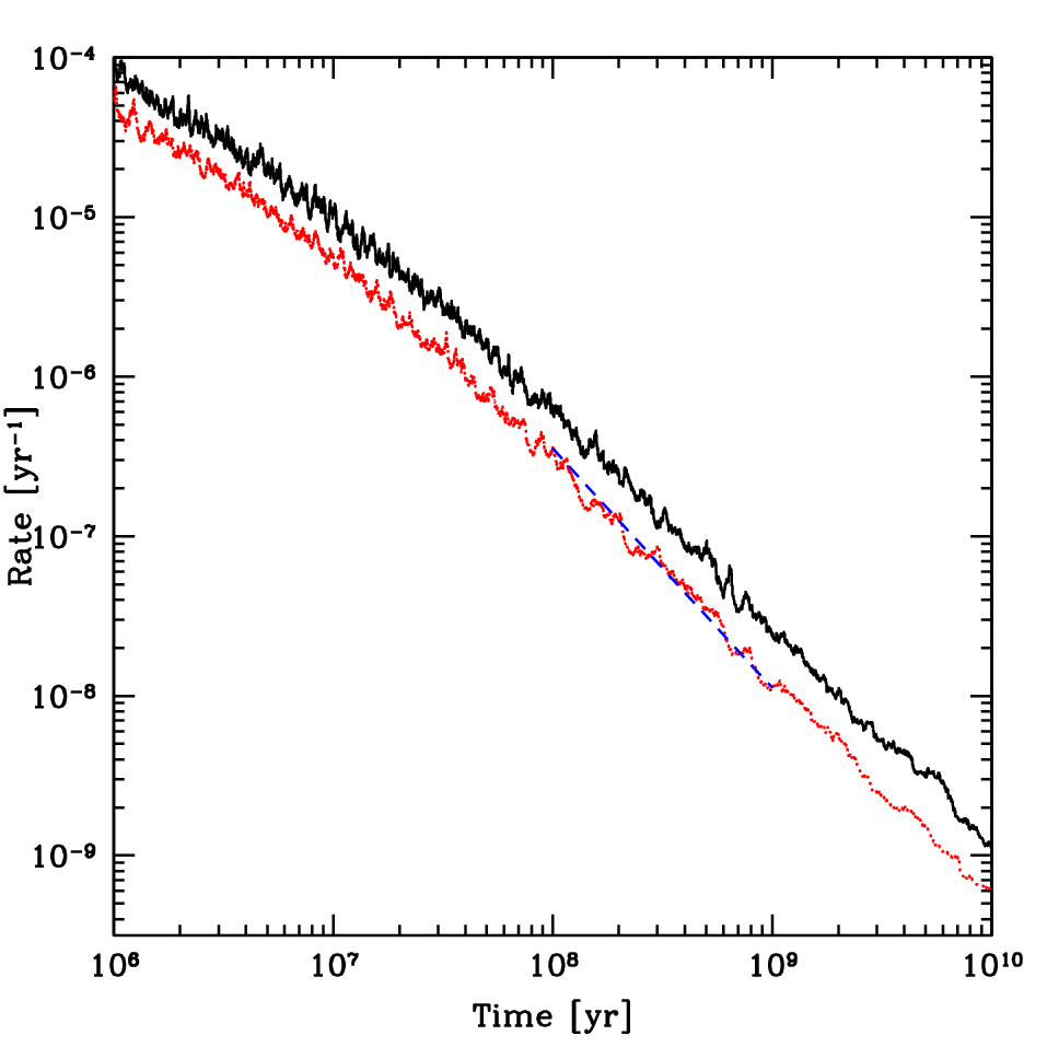
A star will be tidally disrupted by the BH if it comes within a radius . Using this criterion, we remove stars that are disrupted by the black hole, and add their mass to the black hole. In Figure 3, we plot the average tidal disruption rate of stars in Models I & II as a function of time. We find that after the first relaxation timescale, the time evolution of the disruption rate is well approximated as a power-law .
If a star has a small enough angular momentum such that its pericenter distance is less than the tidal disruption radius, it will be disrupted in less than one orbital period. Therefore, the tidal disruption rate is determined by the flow of stars into the empty loss-cone66 6 The stars can also diffuse to higher specific energy, however the fractional change in energy required is usually much larger than the fractional change in angular momentum.. The stars can diffuse into the loss-cone through regular two-body relaxation, large-angle scattering, or coherent effects such as resonant relaxation (Rauch & Tremaine, 1996; Rauch & Ingalls, 1998). We can hope to determine the primary mechanism behind loss-cone refilling using the time evolution of the system (i.e., ).
The diffusion rate of stars into the empty loss-cone from two-body relaxation scales approximately as . After the cluster begins to expand, the cluster should expand such that the relaxation timescale follows the clusters age, . Thus the rate of tidal disruptions from regular relaxation is , in agreement with our results. Large-angle scattering will disrupt stars with a similar dependence on time, but at a rate reduced by .
For resonant relaxation, the tidal disruption rate should be , where is the resonant relaxation timescale, and normalizes the rate and can be determined using numerical simulations (Rauch & Ingalls, 1998; Hopman & Alexander, 2006a; Komossa & Merritt, 2008; Eilon et al., 2009). If we exclude general relativistic precession, the resonant relaxation timescale is determined by the precession of stars from their own self-gravity, and scales roughly as , independent of the density profile of the stars. For a homologously expanding cluster around a black hole, the radius that encloses a fixed number of stars scales as (see § 2.2.1). Assuming that the orbits are nearly Keplerian, , the disruption rate from resonant relaxation will scale as , the same as for regular relaxation. As can be seen in Figure 3, the tidal disruption rate scales as after , when the cluster begins to expand. From scaling arguments alone, we can not determine the relative contribution of tidally disrupted stars from resonant relaxation or regular relaxation. Resonant relaxation should be more important on these scales since the total enclosed mass in stars is much less than the BH mass. However, artificial numerical precession can prevent resonant relaxation from occurring in numerical simulations.
To determine the cause of the tidal disruption events we can analyze the tidal disruption rates dependence on . For resonant relaxation the disruption rate scales as , whereas for regular relaxation the rate scales as . Following Komossa & Merritt (2008), we have performed smaller numerical simulations for recoiling star clusters with varying . These simulations had only of initial stars on an density profile. This profile was chosen so that the regular relaxation timescale was shortest at largest radii. The tidal disruption rate as a function of time and mass is shown in Figure 4. Despite the stochastic variations given the small number of stars, we see that the tidal disruption rate scales approximately as at early times, and falls off as after approximately one relaxation timescale of the system (). We have confirmed that the disruptions are indeed caused by resonant effects by observing that the stars that are disrupted are preferentially from the inner most region of the cusp, and undergo angular momentum evolution on a timescale much shorter than the relaxation timescale.
Because the timescale of large-angle scattering ejecting stars is also proportional to the relaxation timescale, both the tidal disruption rate and ejection rate have the same functional dependence on time. By the end of the simulations, approximately of the stars are disrupted by the BH. This is inconsistent with the results of Lin & Tremaine (1980) who found that the BHs in globular clusters are more efficient at ejecting stars from density cusps than consuming them. However, here we are analyzing only a fraction of the entire density cusp.

The tidal disruption of a star from an offset BH is an exciting possibility for detecting recoiled BHs (Komossa & Merritt, 2008). Previous work has so far focused on the disruption of stars from clusters that were recently ejected by merger (Komossa & Merritt, 2008), as it was thought that the tidal disruption rate would decline exponentially with time. This is in contrast with the power-law decline in tidal disruptions found here. Although the tidal disruption rate peaks early in the cluster evolution, most recoiled BHs are ejected from their host galaxy in the early Universe. Taking the time evolution of the clusters from equation (4), the tidal disruption rate of stars in a cluster today is approximately
| (6) |
for each cluster with and . In Paper I, we found that there are perhaps tens of clusters with , and hundreds with around each Milky Way like galaxy. Thus, per Milky Way galaxy, the tidal disruption rate of stars by rogue BHs is approximately () for (). This is somewhat lower than the estimated tidal disruption rate of stars by BHs that reside in galaxies . Upcoming optical surveys, such as PTF77 7 http://www.astro.caltech.edu/ptf/, Pan-STARRS88 8 http://pan-starrs.ifa.hawaii.edu/, and LSST99 9 http://www.lsst.org/ are most sensitive to flares from BHs (Strubbe & Quataert, 2009), precisely the range of BHs we expect to have the highest present day tidal disruption rates. These events can be identified as off-nuclear flares, which have broad emission lines with a mean redshift comparable to their nearby galaxies1010 10 Because the recoiling clusters are completely in the empty loss cone regime, the typical pericenter distance of the tidally disrupted star in a recoiled star cluster is always close to . This may result in a qualitatively different flare than associated with a central black hole.. Tidal disruption flares from low mass recoiled BHs may be a promising avenue for detecting these unique systems.


2.2.3 Present State of Star Clusters
The purpose of these long-term -body simulations is to determine the present day distribution of stars around recoiled BHs, with the goal of optimizing the search strategies for these clusters in § 4. In Figure 5, we plot the average projected number of stars enclosed within a radius from the BH. In addition, we plot the results of our Fokker-Planck simulations from § 3 and Paper I, rescaled in the final number of stars to match the -body simulations. The stars in the -body simulations are distributed with the same functional form and slope with near the half mass radius, as we found in our initial simulations, despite the total number of stars being of that found in Paper I. Regular relaxation, which was included in Paper I, appears to determine the shape and expansion of the cluster, whereas a combination of strong-encounters between stars and the tidal disruption of stars from resonant relaxation, neither of which were included in our Fokker-Planck simulations of Paper I, determine the final number of stars in the cluster. We conclude from this agreement that recoiled clusters of comparable mass stars have power-law density profiles with .
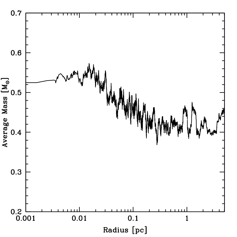
We find only moderate evidence of mass-segregation in these clusters, even though the stars spanned a factor of in mass, as shown in Figure 6. In our analysis of Model II, we binned the stars into shells around the BH, and found that the average mass of stars in each shell decreased as a shallow power-law of radius from and . Because the massive stars are more luminous, this segregation will steepen the light density profile in the cluster.
To check the robustness of our results on the underlying assumptions of our simulations, we have run additional simulations that i) start with a shallower density profile, ii) include stellar evolution, iii) include general relativistic effects to 2.5 post-Newtonian order, iv) have a significantly smaller loss-cone, or v) use a significantly different mass function. In cases (i) – (iv) there was no discernible effect on the stellar density distribution or final number of stars in the simulations. In case (v), where the average stellar mass was ten times larger, the cluster dissolved in less than . This simulation started with 190 stars in orbit around the black hole. At the end of the simulation, only two bound stars remained.
3 Fokker-Planck Simulations
We found in our direct -body simulations that only of stars initially bound to a recoiled BHs remained after . In contrast, our time-dependent Fokker-Planck simulations in Paper I, had little mass loss. Nevertheless, the -body simulations and our results from Paper I agree on the shape and slope of recoiled clusters. The -body simulations show that strong encounters between stars as well as an enhanced tidal disruption rate drive the evaporation of the cluster on timescales much shorter than standard, uncorrelated perturbative encounters (Henon, 1969; Lin & Tremaine, 1980). Here we reintroduce the time-dependent Fokker-Planck equation for stars around a central massive object, as originally derived by Bahcall & Wolf (1976), with the addition of two new sink terms in order to account for mass loss caused by strong encounters and resonant relaxation.
Following (Bahcall & Wolf, 1976), we define the relaxation timescale of the initial cluster to be
| (7) |
where is the stellar velocity dispersion after the galaxies merge, is the average stellar mass, is the number density of stars at , and is the standard Coulomb logarithm. In the dimensionless units of time, , and energy, , the time-dependent Fokker-Planck equation reduces to
| (8) |
where is the dimensionless distribution function of the stars, is the rate at which stars flow to higher energies, is the tidal disruption rate of stars that diffuse into the BH loss cone via regular two-body relaxation (Bahcall & Wolf, 1977), is the tidal disruption rate of stars that fall into the BH loss cone via resonant relaxation (Rauch & Tremaine, 1996; Rauch & Ingalls, 1998; Hopman & Alexander, 2006a), and the rate that stars are ejected from the cluster owing to strong encounters. Bahcall & Wolf (1976); Bahcall & Wolf (1977) found that
| (9) |
and
| (10) |
where , and where is the maximum specific energy of a star before tidal disruption.
In systems with nearly Keplerian orbits, torques between the stars add coherently, and can efficiently randomize the angular momentum of the stars on a timescale much shorter than the regular (non-coherent) relaxation time. This process, known as resonant relaxation (Rauch & Tremaine, 1996), can lead to an enhanced rate of tidal disruptions as the stars enter the loss cone (Rauch & Ingalls, 1998). We follow Hopman & Alexander (2006a), who derived an approximate expression for the resonant relaxation driven tidal disruption rate for Eq. 8. They found that the rate is approximately
| (11) |
where is an unknown efficiency factor of order unity, and is the resonant relaxation timescale. In our numerical simulations we do not include general relativistic precession1111 11 In § 2.2.3, we have included general relativistic precession and found no quantitative different in the tidal disruption rate or the distribution of stars in the cluster, so the only form of precession that limits the resonant relaxation is caused by the enclosed mass of the system. In these circumstances Hopman & Alexander (2006a) found .
Although strong encounters are less important in calculating the flow of stars to higher and lower energies, in eq. (9), a single strong encounter can eject a star from the cluster. Henon (1969) first calculated the escape rate of stars from isolated star clusters for an arbitrary distribution of stars. Lin & Tremaine (1980) extended this work to stars around a central point mass. They found that strong encounters are important in calculating the flux of stars out of the cusp, as confirmed in our -body experiments in § 2. By changing the limits of integration in equation (35) of Lin & Tremaine (1980), we derive the rate that equal-mass stars are ejected from the cluster as a function of energy,
| (12) |
where is the negative specific energy required to be ejected. Note that in our dimensionless units, equation (12) is suppressed by the Coulomb logarithm , compared to the rest of equation (8).
We determine the time evolution of the cluster by numerically solving equation (8) with the boundary conditions and until , at which point we set . We remove stars from the kick by scaling the distribution function of stars as , where . This yields an asymptotic density profile with for , as expected immediately after the kick (Komossa & Merritt, 2008). We use a variety of , 0.1, 0.25, 0.5, 1.0, 2.0, 10.0, to explore the importance of in matching the number of stars in § 2, as well as to explore the uncertainty in the efficiency of resonant relaxation. In all of our calculations we set .
3.1 Fokker-Planck Results
In our calculations, we find reasonable agreement between the -body simulations and the numerical solution of the Fokker-Planck equation only when we include a new sink term, , which accounts for the tidal disruption of stars owing to resonant relaxation. We find the best agreement when we set the resonant relaxation parameter . When we exclude resonant relaxation, as we did in Paper I, we only get the proper functional form of the -body solution to the density profile, but not the proper number of stars. Without resonant relaxation, the Fokker-Planck simulation expand too rapidly at the half-mass radius. Indeed, when comparing the radii that enclose the inner 1, 10, or 100 stars of the Fokker-Planck simulations to the -body simulations we find complete agreement that the cluster expands self-similarly as (see the discussion in § 2.2.1). At the radius that encloses half of the cluster mass, we find the Fokker-Planck simulations still scale as , and the -body simulations scales as . The scaling is in agreement with our expectation that the relaxation timescale should be approximately the age of the cluster (Paper I).
Resonant relaxation reconciles the two fundamental differences between our previous Fokker-Planck simulations and our current -body simulations. Resonant relaxation destroys stars at a faster rate than regular relaxation, reducing the number of stars in the cluster. As a consequence of the depleted stars, the outer cluster expands more slowly, matching the N-body simulations. In Figure 5, we plot the enclosed mass profile of the clusters from our -body simulations, along with our Fokker-Planck simulations including and excluding resonant relaxation (with ). Resonant relaxation reduces the number of stars in the simulation to the correct value. Although including resonant relaxation in the Fokker-Planck simulations does give a similar mass density profile, there are too few stars in the inner most region. Unfortunately, the Fokker-Planck simulations are one-dimensional, and can not take into account the anisotropy that must develop as the cluster expands, or the preference to deplete eccentric orbits near the black hole.
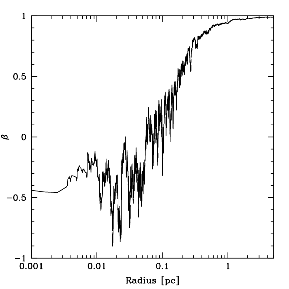
The anisotropy of the cluster is often measured by the parameter
| (13) |
where is the radial velocity dispersion of the system, and is the one-dimensional tangential velocity dispersion, such that . For an isotropic cluster, and . A cluster with stars on only radial orbits will have . We plot the anisotropy of the -body simulations as a function of radius in Figure 7. The cluster shows a large degree of anisotropy at nearly all radii. From the innermost stars outward, the stars in the cluster change from preferentially tangential orbits () to radial orbits (). Indeed, the development of anisotropy is a natural consequence of the conservation of angular momentum in a Keplerian potential. As the cluster expands, the outermost stars must be on more radial orbits. The innermost stars, on the other hand, have their eccentric orbits depleted when they are tidally disrupted by the BH. In the our one dimensional Fokker-Planck simulations, we assume isotropy, which effectively relaxes the angular momentum of the stellar population on a timescale much shorter than the actual relaxation timescale. This causes the cluster to disrupt stars very close to the black hole, that would otherwise remain on circular orbits. This scenario can be tested with an appropriate two dimensional Fokker-Planck code (Cohn, 1980; Takahashi, 1995; Drukier et al., 1999, e.g.,), extended to include the effects of resonant relaxation. Despite the anisotropy of the cluster, the density profile predicted by the Fokker-Planck simulations matches the -body simulations remarkably well, except in the innermost region of the cusp.
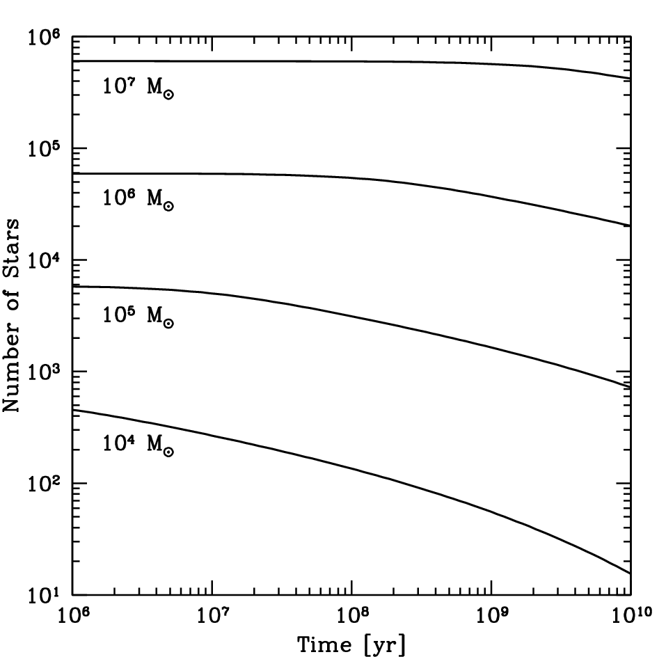
The -body simulations of § 2 are computationally challenging given the long timescale of the calculation and can not be easily extended to larger star clusters. Solving the Fokker-Planck equations, however, does not depend on . Rather, it is calculated on a fixed grid in energy space, and takes only a short computational time to complete. We therefore use the Fokker-Planck code to compute the evolution of more massive recoiled star clusters around , , and , all with kick velocity scaled to their respective velocity dispersion, , and normalized by the relation. We set the free parameters and , which give comparable time evolution to the -body simulations in § 2. In Figure 8, we plot the number of stars as a function of time for these recoiled clusters. We find that the evolution of star clusters around black holes with , lose less than of their mass over . For the largest black holes with , the clusters lose negligible mass over the age of the universe. We can therefore expect that the most massive clusters represent the conditions of the stellar cusp when they were recoiled from their parent galaxy.
We find that the total number of stars at the end of the simulations is only weakly dependent on the value we choose for . Indeed, over two orders of magnitude in , the final number of stars in the cluster changed by only . This is because for most of the range of values, the corresponding velocity for stars ejected with energy , was less than mean ejection velocity as seen in Figure 2. In the limit , equation (12) goes to zero, and we recover the results of our simulations from Paper I. Unfortunately, we can not use these simulations to calibrate for BHs in galactic nuclei, where there is a reservoir of stars outside of . When , equation (12) is not accurate because it does not account for the flux of stars to lower energy states from outside of the cusp or the return of stars that are still bound to the cusp of stars (Lin & Tremaine, 1980).
The evolution of the star clusters is sensitive to the value of . For sufficiently small, , clusters of stars around BHs only lose of their mass over . Likewise, for , the cluster loses mass so rapidly, that it has star after . Such a scenario may represent a cluster with high concentration of stellar mass black holes.
4 Photometric Properties of Old Clusters
SDSS DR7 (Abazajian et al., 2009) has unique photometric objects that we would like to sort through in order to find candidate recoiled star clusters. Our goal is to develop the most general photometric model possible for recoiled star clusters in SDSS, while eliminating false positives as efficiently as possible. Generally, we expect the clusters to contain as few as stars for the smallest BHs , up to stars for the most massive BH in the halo . These clusters should have a power-law density profile with , but certainly , which corresponds to a cusp of stars which flows away from the BH. Since the Milky Way has not had a recent major merger, we expect the clusters to be old. In this section, we develop such a model, focusing on the photometric properties of a stochastic cluster of old stars with a power-law density profile. Their spectra should indicate a large for clusters around the most massive BHs, and large mass-to-light ratio at redshift , but we focus on photometric identification of candidates for spectroscopic follow-up.
4.1 Cluster Models
We generate model star clusters by randomly selecting stars from a Kroupa initial mass function of stars (Kroupa & Weidner, 2003) using two main modes of star formation. For Model A, we assume that the stars formed continuously in time with a constant star formation rate until the BH was ejected after . This is consistent with the estimated star formation history of the MW galactic center (Alexander & Sternberg, 1999; Genzel et al., 2003). We contrast this with Model B, where the stars formed simultaneously with the BH merger, as galaxy mergers are often associated starbursts. In all instances we assume that the time between the merger of the galaxy and the merger of the BHs is negligible.
The precise photometric properties of the stars depends on their metallicity and age. We consider three different metallicity histories of stars: (I) solar metallicity (), (II) sub-solar metallicity (), and (III) the estimated time evolution of metallicity of the galactic center.
In all of our calculations we use the online single star population synthesis code BaSTI1212 12 Available at http://astro.ensc-rennes.fr/basti/synth_pop/index.html (Pietrinferni et al., 2004; Cordier et al., 2007), and convert all observables to the SDSS color system using Table 1 of Jester et al. (2005). The typical uncertainty in the colors from our conversion scheme is much smaller than the intrinsic variation in the colors of the star clusters.
In Figure 9, we plot a color-color diagram of our Model Clusters with , and after ejection. Overall, the loci of star clusters follow the distribution of galactic stars identified by SDSS, however, they visually appear to be well separated from SDSS galaxies. In the figure, it is clear that many clusters contain a star on the giant branch. Because such stars are more luminous than all of the other stars in the cluster, these systems are likely indistinguishable from the population of late-type stars in the halo. Clusters with follow a similar distribution.


Because the star clusters can not be distinguished from individual stars based on their colors alone, a successful photometric search needs to exclude point sources, and use a magnitude system which doesn’t depend on the exact light profile of the object. We therefore focus on the photometric properties of resolved objects, using the Petrosian magnitude system (Blanton et al., 2001; Yasuda et al., 2001). This system is is defined by the Petrosian ratio,
| (14) |
where is azimuthally averaged surface brightness profile in any particular band. The Petrosian radius, , is defined by in the SDSS system. The total Petrosian flux (and magnitude) from the object is calculated as the total integrated light within , where is determined in the -band alone.
We use the azimuthally averaged cumulative light profile to distinguish candidates from galaxies and point sources. The SDSS catalog has the mean flux of light in annuli around the peak of the photometric object. We add the light in these annuli to recreate the total amount of light within radii arcsec. We use these bins to calculate the logarithmic slope of the cumulative light profile, , For a completely resolved star cluster with power-law density profile , we expect the light profile to approach where . Outside the half-light radius of the cluster, however, the slope of the profile changes significantly from a single power-law. To model this we use the distribution of stars from our -body simulations and generate mock light density profiles with a variety of PSFs and angular sizes. To facilitate the search in § 5, we have split our mock profiles into bins of varying . The best fit parameters are detailed in Table 1.
| (arcsec) | ||||
|---|---|---|---|---|
| 2.0–3.0a | 0.78 – 0.88 | … | … | … |
| 2.0–3.2b | … | … | ||
| 3.0–4.5 | … | 0.25 – 0.5 | 0.10–0.25 | … |
| 4.0–6.0 | … | 0.35 – 0.70 | 0.28 – 0.45 | 0.1 – 0.2 |
5 Photometric Search
SDSS has imaged approximately one quarter of the sky to a limiting magnitude . As the largest database of photometric and spectroscopic objects in the sky , it presents a prime opportunity to search for recoiled clusters. In § 4.1 we developed a simple photometric model of recoiled star clusters in Milky Way like galaxies. Here we use this model to systematically search for photometric candidates in SDSS DR7.
We use the SDSS DR7 CasJobs1313 13 Located at http://casjobs.sdss.org/CasJobs/ photometry database to select objects by size, shape, color, and azimuthally averaged light profile. We limit our search to resolved objects with a Petrosian radius in the band.
Our color selection criteria is illustrated by the trapezoids in Figure 9. We use the Petrosian magnitude system color corrected for extinction (Schlegel et al., 1998). Our criteria focus on an old population of metal-poor to solar metallicity stars but excludes clusters with a star on the red giant branch. We choose our candidate clusters out of the parallelogram defined by , . Additionally, we require that the shape of the candidates be circular by selecting for objects with ratio of semi-minor to semi-minor axes greater than . These criteria select resolved photometric objects as candidate recoiled clusters, with photometric properties of stars. We limit our sample further by using the azimuthally averaged cumulative light profile () of the remaining objects as detailed in Table 1. In addition we search for simpler model clusters with and between 0.6 and 0.9.
Using these criteria, we are left with candidates, which we visually inspect to remove obvious interlopers. These tend to be individual or binary stars in crowded fields, face-on disk galaxies, and cuspy elliptical galaxies. We are left with objects, which we list in Tables 2 & 3. Thumbnails of a selection of candidates is shown in Figure 10. The number of candidates that remain is likely a reflection of our ability to visually inspect the candidates. It is impossible to visually inspect the objects selected through color alone, and we had to use some model dependent choices for the light profile to obtain a more reasonable number of photometric candidates ().
| Object | |||
|---|---|---|---|
| SDSS J003550.53-100543.0 | 19.57 | 19.10 | 3.07 |
| SDSS J005248.49+155331.6 | 19.81 | 18.99 | 3.24 |
| SDSS J011023.54-090416.1 | 19.70 | 19.31 | 3.19 |
| SDSS J015724.63-085424.1 | 18.48 | 18.19 | 3.30 |
| SDSS J020705.55+003738.9 | 19.81 | 19.29 | 3.49 |
| SDSS J021500.57+001217.8 | 20.40 | 19.77 | 3.57 |
| SDSS J030347.44-081909.5 | 20.12 | 19.01 | 3.21 |
| SDSS J064325.65+281559.3 | 20.51 | 19.80 | 2.79 |
| SDSS J073940.32+221323.1 | 18.67 | 18.39 | 4.49 |
| SDSS J074214.49+251424.0 | 20.14 | 19.35 | 2.94 |
| SDSS J074827.56+261836.6 | 19.74 | 19.04 | 3.09 |
| SDSS J075550.27+343959.3 | 20.51 | 19.89 | 3.09 |
| SDSS J080005.57+514410.6 | 20.68 | 19.57 | 3.44 |
| SDSS J081020.09+315018.6 | 20.72 | 19.93 | 2.75 |
| SDSS J081546.83+155039.8 | 20.32 | 19.88 | 2.71 |
| SDSS J082724.19+340543.7 | 19.77 | 19.23 | 3.43 |
| SDSS J083158.70+332233.5 | 19.35 | 18.88 | 3.01 |
| SDSS J083701.15+230023.2 | 20.54 | 20.20 | 2.56 |
| SDSS J084034.69+162319.5 | 20.13 | 19.62 | 3.06 |
| SDSS J084246.26+361533.7 | 19.66 | 19.09 | 4.00 |
| SDSS J084505.56+451932.0 | 20.59 | 20.11 | 3.35 |
| SDSS J084647.94+001638.4 | 21.07 | 20.44 | 3.43 |
| SDSS J092335.02+472837.1 | 19.64 | 19.01 | 2.99 |
| SDSS J092607.17+021555.4 | 20.39 | 19.60 | 3.28 |
| SDSS J092757.48+054543.7 | 20.03 | 19.22 | 3.12 |
| SDSS J092921.02+545144.3 | 19.31 | 18.97 | 3.25 |
| SDSS J093815.82+231234.8 | 20.10 | 19.19 | 3.06 |
| SDSS J094801.22+324203.4 | 19.72 | 19.13 | 3.02 |
| SDSS J101754.64+803827.9 | 20.02 | 19.14 | 3.59 |
| SDSS J104012.45+183600.5 | 19.71 | 19.17 | 3.12 |
| SDSS J104012.45+645611.0 | 20.20 | 19.45 | 3.13 |
| SDSS J104700.20+451459.4 | 19.95 | 19.24 | 3.31 |
| SDSS J105840.27-012816.9 | 20.53 | 19.71 | 2.99 |
| SDSS J105846.93+170430.1 | 19.07 | 18.37 | 3.19 |
| SDSS J105907.75-031445.6 | 19.60 | 18.67 | 3.48 |
| SDSS J111223.68+072718.0 | 19.23 | 18.70 | 3.87 |
| SDSS J111327.28+081717.1 | 18.88 | 18.55 | 4.30 |
| SDSS J112142.07+182723.3 | 19.53 | 19.12 | 3.23 |
| SDSS J112711.19+113814.8 | 20.14 | 19.24 | 3.54 |
| SDSS J113013.20+643939.4 | 18.99 | 18.72 | 3.76 |
| SDSS J113137.97+172219.0 | 19.49 | 18.66 | 3.49 |
| SDSS J113308.62+002113.2 | 20.84 | 19.71 | 2.82 |
| SDSS J114546.59+081137.7 | 19.67 | 19.08 | 3.87 |
| SDSS J115108.59+030704.8 | 19.63 | 19.33 | 2.92 |
| SDSS J115253.98+171842.6 | 20.00 | 19.27 | 2.92 |
| SDSS J115526.94+355320.0 | 19.95 | 19.55 | 3.01 |
| SDSS J115543.73+333639.9 | 18.83 | 18.39 | 4.43 |
| SDSS J115957.30+020749.5 | 19.72 | 19.14 | 3.27 |
| SDSS J120446.11+270030.1 | 19.94 | 19.42 | 3.06 |
| SDSS J120533.94+022352.9 | 20.13 | 19.28 | 3.11 |
| Object | |||
|---|---|---|---|
| SDSS J120648.21+450646.7 | 21.06 | 20.08 | 3.16 |
| SDSS J121700.34+353542.1 | 20.38 | 19.74 | 3.22 |
| SDSS J123544.93+193016.9 | 20.55 | 19.87 | 2.84 |
| SDSS J123614.93+013708.7 | 20.27 | 19.81 | 3.03 |
| SDSS J125011.62-021800.1 | 21.16 | 20.51 | 2.65 |
| SDSS J125734.92+253916.5 | 20.49 | 19.92 | 2.78 |
| SDSS J125915.28+070342.6 | 20.01 | 19.52 | 3.30 |
| SDSS J125958.63-002508.4 | 19.75 | 18.71 | 3.26 |
| SDSS J130109.32+462607.1 | 21.28 | 20.15 | 2.76 |
| SDSS J130153.77+504842.2 | 20.38 | 19.64 | 2.85 |
| SDSS J130154.22-031323.3 | 19.67 | 18.97 | 3.32 |
| SDSS J132249.56+084115.6 | 19.85 | 19.22 | 3.27 |
| SDSS J132610.71+535511.7 | 20.79 | 20.26 | 3.24 |
| SDSS J133057.40+184836.7 | 20.00 | 19.28 | 2.66 |
| SDSS J133212.59+353159.7 | 19.56 | 18.94 | 2.93 |
| SDSS J134127.13+081550.6 | 21.56 | 20.52 | 2.06 |
| SDSS J134459.96+030428.6 | 19.76 | 19.55 | 3.13 |
| SDSS J134737.53+203427.0 | 20.19 | 19.78 | 2.94 |
| SDSS J134852.16+245743.4 | 19.72 | 19.16 | 3.77 |
| SDSS J135040.46+103538.7 | 20.75 | 19.95 | 2.84 |
| SDSS J135241.53+121430.8 | 20.51 | 19.66 | 3.06 |
| SDSS J135544.47-065531.4 | 20.29 | 19.54 | 2.90 |
| SDSS J140113.91+060627.7 | 20.13 | 19.71 | 2.85 |
| SDSS J141327.28+282847.1 | 19.58 | 18.79 | 3.05 |
| SDSS J141418.26+454312.8 | 18.94 | 18.57 | 4.37 |
| SDSS J142920.56+261616.5 | 20.13 | 19.39 | 2.80 |
| SDSS J142935.43+073722.6 | 19.59 | 18.87 | 3.18 |
| SDSS J145030.79+380441.6 | 19.62 | 19.06 | 2.91 |
| SDSS J145145.53+103402.0 | 19.94 | 19.32 | 3.45 |
| SDSS J145150.02+352929.8 | 20.03 | 19.53 | 2.78 |
| SDSS J145345.50+080808.7 | 20.37 | 19.58 | 3.03 |
| SDSS J150113.32+051304.1 | 19.92 | 19.37 | 2.91 |
| SDSS J150459.72+081819.7 | 20.50 | 19.89 | 2.78 |
| SDSS J151934.33+134102.8 | 20.51 | 20.12 | 3.33 |
| SDSS J152006.92+085031.0 | 20.45 | 19.68 | 2.78 |
| SDSS J152249.28+473700.1 | 20.31 | 19.82 | 3.12 |
| SDSS J152646.00+210607.1 | 21.21 | 19.97 | 3.33 |
| SDSS J153145.65+150057.6 | 20.12 | 19.54 | 3.11 |
| SDSS J155333.07+423146.0 | 20.25 | 19.53 | 3.07 |
| SDSS J155442.55+055111.1 | 19.09 | 18.60 | 3.23 |
| SDSS J160630.13+351046.2 | 19.48 | 19.06 | 3.04 |
| SDSS J160702.48+110353.3 | 20.27 | 19.78 | 3.89 |
| SDSS J162536.57+563531.9 | 20.99 | 19.96 | 3.53 |
| SDSS J163339.07+132635.6 | 20.23 | 19.56 | 3.46 |
| SDSS J163659.29+235816.2 | 20.05 | 19.01 | 2.93 |
| SDSS J170525.39+235241.5 | 19.17 | 18.37 | 4.08 |
| SDSS J172243.89+080447.8 | 20.44 | 19.97 | 2.91 |
| SDSS J210803.13-001350.4 | 20.35 | 19.52 | 3.15 |
| SDSS J213035.54-070545.7 | 20.76 | 20.05 | 3.19 |
| SDSS J215424.98+002023.4 | 20.01 | 19.14 | 3.23 |
| SDSS J233106.11+075810.9 | 20.89 | 19.99 | 2.97 |
| Object | |||
|---|---|---|---|
| SDSS J084822.47+355630.4 | 18.69 | 18.21 | 3.60 |
| SDSS J045505.26+244156.3 | 21.06 | 19.43 | 2.94 |
| SDSS J114607.52+135233.1 | 20.57 | 19.81 | 2.53 |
| SDSS J090546.22+225309.9 | 20.50 | 19.77 | 2.88 |
| SDSS J102509.23+215445.8 | 20.22 | 18.86 | 3.84 |
| SDSS J211006.40+002759.2 | 19.18 | 18.60 | 3.32 |
| SDSS J100310.59+282625.0 | 18.86 | 18.05 | 3.45 |
| SDSS J121414.73+161215.4 | 19.15 | 18.22 | 3.63 |
| SDSS J051413.98+164920.2 | 18.95 | 17.89 | 3.41 |
| SDSS J161526.75+110822.9 | 21.62 | 20.84 | 2.37 |
| SDSS J052222.65-013302.9 | 20.16 | 19.17 | 2.77 |
| SDSS J135018.11+092421.7 | 18.89 | 17.90 | 3.79 |
| SDSS J003209.31+071259.2 | 18.94 | 17.80 | 5.22 |
| SDSS J144115.60+185843.8 | 20.12 | 19.26 | 3.46 |
| SDSS J160236.41+322318.7 | 19.88 | 18.75 | 2.87 |
| SDSS J163339.50+440918.3 | 20.02 | 18.98 | 2.57 |
| SDSS J132908.57+232303.8 | 19.62 | 18.46 | 3.09 |
| SDSS J144856.99+153744.6 | 20.39 | 19.54 | 2.81 |


6 Spectroscopic Search
The selection of spectroscopic objects in SDSS DR7 is not ideal for serendipitously locating the star cluster around a recoiled BH. Indeed, many of the main science objectives for spectroscopic targets specifically exclude objects with the photometric properties similar to the recoiled clusters we search for. Nevertheless, resolved recoiled clusters would be identified in SDSS photometrically as a galaxy because of its extended size, but unlike galaxies, would have an extremely low redshift, .
We use SDSS spectroscopy to select candidate clusters by their identified redshift with , corresponding to radial velocities with magnitude less than . To exclude single and unresolved binary stars, we restrict our results to objects with Petrosian radii, in both the and bands. We then remove blended objects, which are mostly galaxies with foreground stars. This results in approximately objects identified by SDSS photometry as galaxies, and identified as stars. We have visually inspected all objects. All of the remaining objects in the sample have two main features: (i) a star like object on a diffuse source or (ii) featureless and diffuse source. In case (i), the spectral identification of the source is always stellar. The majority of objects that fall into category (ii) were incorrectly identified with . The remaining cases were not spherical in shape or clumpy, and therefore not classified as recoiled cluster candidates.
7 Literature Search
We have also explored the literature for galaxies that were spectroscopically identified as stars owing to their low redshift. Sargent (1970) took low-dispersion spectra of 141 objects selected from Zwicky’s catalogs of compact galaxies (Zwicky & Zwicky, 1971, available in), and found that 14 objects had near-zero redshifts and identified the galaxies as having a foreground star. We have reanalyzed newer digital images and spectra of these objects. In some cases the foreground star has moved and new spectra show the objects are extragalactic. However, most were visually identified as galaxies because of their disk like shape. Only one object, IV Zw 26, could not be excluded as a candidate owing to insufficient resolution in any survey.
8 Summary and Conclusions
We have followed the long term evolution of star clusters around recoiled BHs using long term -body simulations, with a one-to-one correspondence between the stars and -body particles. We have found that for , of the stars are ejected from the star cluster, and of the stars are tidally disrupted by the central BH within . We have scaled these results to BHs with masses , finding that stars remain around the BH today for a typical recoiled BH. For more massive BHs, the cluster should eject or disrupt few stars over . Although a single BH has a small tidal disruption rate, we have found that the total rate for all clusters in Milky Way like galaxies is , which is only a factor of lower than expected in the galactic center. We have extended our one-dimensional Fokker-Planck treatment in Paper I to include resonant relaxation and large-angle scattering to account for the dominate mass loss mechanisms of the cluster. Using this treatment, we were able to get satisfactory agreement between the -body simulations and Fokker-Planck simulations. Some discrepancy remained, which we attribute to the large amount of anisotropy in realistic clusters.
We used our -body simulations to generate random realizations of star clusters today, which guided our search for star clusters around recoiled BHs in SDSS. In our photometric search through SDSS data, we assumed that the star clusters have a power-law density profile and that they have colors comparable to an old population of stars. We used these criteria to find candidates of which only had a light density profile out to consistent with a recoiled star cluster with power-law density slope. We visually inspected all candidates, and found that many were the bulges of nearby face-on spirals. The remaining candidates were faint, and difficult to distinguish from distant galaxies. Follow-up spectroscopy is necessary to identify their nature. If any of them are a star cluster around a recoiled BH, it would show unusually high velocity dispersion at , with a spectrum of a population of old stars.
We also searched the spectroscopic database of SDSS for resolved objects with a low redshift/blueshift consistent with the Local Group. The vast majority of these candidates were galaxies with bright foreground stars. We found no candidates that appeared to be a recoiled cluster.
The criteria we used to search for candidate clusters required the cluster to have a well defined power-law density profile, as found in our numerical simulations. Because we did not include compact remnants in our simulations (which would have the correct density profile but not light profile) we can not be confident that we properly included all star clusters in our search. Unfortunately, most research on stellar remnants around supermassive black holes focus on mass segregation around relaxed stellar cusps (Freitag et al., 2006; Hopman & Alexander, 2006b; O’Leary et al., 2009; Alexander & Hopman, 2009; Keshet et al., 2009). These simulations find that compact remnants play an important role in the dynamics for radii . We have not included these objects because it is difficult to quantify how many compact remnants would be in this region immediately before the binary merges. Indeed, the segregation of the compact remnants can only occur after the low-mass stars populate this region (Merritt, 2009). In future work we hope to include these compact remnants, and extend our Fokker-Planck code to include large angle scattering between stars of multiple masses (O’Leary et al., 2009).
An alternative search strategy, which we did not explore here, is to cross-check less stringent criteria with alternative databases, such as the ROSAT x-ray survey.
Acknowledgments
We thank Warren Brown, Kelly Holley-Bockelmann, Nick Stone, and Matt Walker for their helpful discussions. We thank Wallace Sargent and Francois Schweizer for bringing Zwicky’s catalog to our attention. We thank Ulf Löckmann for publicly releasing his BHint code, as well as the BaSTI group for allowing us to use their code. This project makes use of data products from the Sloan Digital Sky Survey, which is managed by the Astrophysical Research Consortium for the Participating Institutions. This research has also made use of the NASA/IPAC Extragalactic Database (NED) which is operated by the Jet Propulsion Laboratory, California Institute of Technology, under contract with the National Aeronautics and Space Administration. This work was supported in part by NSF grant AST-0907890 and NASA grants NNX08AL43G and NNA09DB30A. Support for the completion of this work was provided to RMO by the National Aeronautics and Space Administration through Einstein Postdoctoral Fellowship Award Number PF0-110078 issued by the Chandra X-ray Observatory Center, which is operated by the Smithsonian Astrophysical Observatory for and on behalf of the National Aeronautics Space Administration under contract NAS8-03060
References
- Abazajian et al. (2009) Abazajian K. N., Adelman-McCarthy J. K., Agüeros M. A., Allam S. S., Allende Prieto C., An D., Anderson K. S. J., et al. 2009, ApJS, 182, 543
- Alexander & Hopman (2009) Alexander T., Hopman C., 2009, ApJ, 697, 1861
- Alexander & Sternberg (1999) Alexander T., Sternberg A., 1999, ApJ, 520, 137
- Amaro-Seoane et al. (2004) Amaro-Seoane P., Freitag M., Spurzem R., 2004, MNRAS, 352, 655
- Bahcall & Wolf (1976) Bahcall J. N., Wolf R. A., 1976, ApJ, 209, 214
- Bahcall & Wolf (1977) Bahcall J. N., Wolf R. A., 1977, ApJ, 216, 883
- Baker et al. (2006) Baker J. G., Centrella J., Choi D.-I., Koppitz M., van Meter J. R., Miller M. C., 2006, ApJ, 653, L93
- Bekenstein (1973) Bekenstein J. D., 1973, ApJ, 183, 657
- Bertone et al. (2005) Bertone G., Zentner A. R., Silk J., 2005, PhRvD, 72, 103517
- Blanton et al. (2001) Blanton M. R., Dalcanton J., Eisenstein D., Loveday J., Strauss M. A., SubbaRao M., Weinberg D. H., et al. 2001, AJ, 121, 2358
- Blecha et al. (2011) Blecha L., Cox T. J., Loeb A., Hernquist L., 2011, MNRAS, pp 38–+
- Blecha & Loeb (2008) Blecha L., Loeb A., 2008, MNRAS, 390, 1311
- Brown et al. (2005) Brown W. R., Geller M. J., Kenyon S. J., Kurtz M. J., 2005, ApJ, 622, L33
- Campanelli et al. (2007a) Campanelli M., Lousto C., Zlochower Y., Merritt D., 2007a, ApJ, 659, L5
- Campanelli et al. (2007b) Campanelli M., Lousto C. O., Zlochower Y., Merritt D., 2007b, Physical Review Letters, 98, 231102
- Cohn (1980) Cohn H., 1980, ApJ, 242, 765
- Cordier et al. (2007) Cordier D., Pietrinferni A., Cassisi S., Salaris M., 2007, AJ, 133, 468
- Drukier et al. (1999) Drukier G. A., Cohn H. N., Lugger P. M., Yong H., 1999, ApJ, 518, 233
- Eilon et al. (2009) Eilon E., Kupi G., Alexander T., 2009, ApJ, 698, 641
- Fitchett (1983) Fitchett M. J., 1983, MNRAS, 203, 1049
- Freitag et al. (2006) Freitag M., Amaro-Seoane P., Kalogera V., 2006, ApJ, 649, 91
- Genzel et al. (2003) Genzel R., Schödel R., Ott T., Eisenhauer F., Hofmann R., Lehnert M., Eckart A., Alexander T., Sternberg A., Lenzen R., Clénet Y., Lacombe F., Rouan D., Renzini A., Tacconi-Garman L. E., 2003, ApJ, 594, 812
- Gieles et al. (2011) Gieles M., Heggie D. C., Zhao H., 2011, MNRAS, 413, 2509
- Goodman (1984) Goodman J., 1984, ApJ, 280, 298
- Gualandris & Merritt (2008) Gualandris A., Merritt D., 2008, ApJ, 678, 780
- Guedes et al. (2010) Guedes J., Madau P., Mayer L., Callegari S., 2010, ArXiv e-prints
- Hénon (1961) Hénon M., 1961, Annales d’Astrophysique, 24, 369
- Hénon (1965) Hénon M., 1965, Annales d’Astrophysique, 28, 62
- Henon (1969) Henon M., 1969, A&A, 2, 151
- Hopman & Alexander (2006a) Hopman C., Alexander T., 2006a, ApJ, 645, 1152
- Hopman & Alexander (2006b) Hopman C., Alexander T., 2006b, ApJ, 645, L133
- Islam et al. (2004a) Islam R. R., Taylor J. E., Silk J., 2004a, MNRAS, 354, 443
- Islam et al. (2004b) Islam R. R., Taylor J. E., Silk J., 2004b, MNRAS, 354, 629
- Jester et al. (2005) Jester S., Schneider D. P., Richards G. T., Green R. F., Schmidt M., Hall P. B., Strauss M. A., Vanden Berk D. E., Stoughton C., Gunn J. E., Brinkmann J., Kent S. M., Smith J. A., Tucker D. L., Yanny B., 2005, AJ, 130, 873
- Keshet et al. (2009) Keshet U., Hopman C., Alexander T., 2009, ApJ, 698, L64
- Komossa & Merritt (2008) Komossa S., Merritt D., 2008, ApJ, 683, L21
- Kroupa (2001) Kroupa P., 2001, MNRAS, 322, 231
- Kroupa & Weidner (2003) Kroupa P., Weidner C., 2003, ApJ, 598, 1076
- Libeskind et al. (2006) Libeskind N. I., Cole S., Frenk C. S., Helly J. C., 2006, MNRAS, 368, 1381
- Lin & Tremaine (1980) Lin D. N. C., Tremaine S., 1980, ApJ, 242, 789
- Löckmann & Baumgardt (2008) Löckmann U., Baumgardt H., 2008, MNRAS, 384, 323
- Loeb (2007) Loeb A., 2007, Physical Review Letters, 99, 041103
- Loeb (2010) Loeb A., 2010, How Did the First Stars and Galaxies Form?. Princeton, NJ, Princeton University Press, 2010
- Madau & Quataert (2004) Madau P., Quataert E., 2004, ApJ, 606, L17
- Merritt (2009) Merritt D., 2009, ArXiv e-prints
- Merritt et al. (2007) Merritt D., Mikkola S., Szell A., 2007, ApJ, 671, 53
- Merritt et al. (2009) Merritt D., Schnittman J. D., Komossa S., 2009, ApJ, 699, 1690
- Merritt & Szell (2006) Merritt D., Szell A., 2006, ApJ, 648, 890
- Micic et al. (2006) Micic M., Abel T., Sigurdsson S., 2006, MNRAS, 372, 1540
- Micic et al. (2008) Micic M., Holley-Bockelmann K., Sigurdsson S., 2008, ArXiv e-prints
- Mii & Totani (2005) Mii H., Totani T., 2005, ApJ, 628, 873
- Morris (1993) Morris M., 1993, ApJ, 408, 496
- O’Leary et al. (2009) O’Leary R. M., Kocsis B., Loeb A., 2009, MNRAS, 395, 2127
- O’Leary & Loeb (2009) O’Leary R. M., Loeb A., 2009, MNRAS, 395, 781
- Peres (1962) Peres A., 1962, Physical Review, 128, 2471
- Pietrinferni et al. (2004) Pietrinferni A., Cassisi S., Salaris M., Castelli F., 2004, ApJ, 612, 168
- Rauch & Ingalls (1998) Rauch K. P., Ingalls B., 1998, MNRAS, 299, 1231
- Rauch & Tremaine (1996) Rauch K. P., Tremaine S., 1996, New Astronomy, 1, 149
- Sargent (1970) Sargent W. L. W., 1970, ApJ, 160, 405
- Schlegel et al. (1998) Schlegel D. J., Finkbeiner D. P., Davis M., 1998, ApJ, 500, 525
- Schnittman (2007) Schnittman J. D., 2007, ApJ, 667, L133
- Schnittman & Buonanno (2007) Schnittman J. D., Buonanno A., 2007, ApJ, 662, L63
- Sijacki et al. (2010) Sijacki D., Springel V., Haehnelt M., 2010, ArXiv e-prints
- Stone & Loeb (2010) Stone N., Loeb A., 2010, ArXiv e-prints
- Strubbe & Quataert (2009) Strubbe L. E., Quataert E., 2009, MNRAS, 400, 2070
- Takahashi (1995) Takahashi K., 1995, PASJ, 47, 561
- Tichy & Marronetti (2007) Tichy W., Marronetti P., 2007, PhRvD, 76, 061502
- Tremaine et al. (2002) Tremaine S., Gebhardt K., Bender R., Bower G., Dressler A., Faber S. M., Filippenko A. V., Green R., Grillmair C., Ho L. C., Kormendy J., Lauer T. R., Magorrian J., Pinkney J., Richstone D., 2002, ApJ, 574, 740
- Volonteri (2007) Volonteri M., 2007, ApJ, 663, L5
- Volonteri & Perna (2005) Volonteri M., Perna R., 2005, MNRAS, 358, 913
- Yasuda et al. (2001) Yasuda N., Fukugita M., Narayanan V. K., Lupton R. H., Strateva I., Strauss M. A., Ivezić Ž., Kim R. S. J., Hogg D. W., Weinberg D. H., Shimasaku K., Loveday J., et al. 2001, AJ, 122, 1104
- Yu & Tremaine (2003) Yu Q., Tremaine S., 2003, ApJ, 599, 1129
- Zwicky & Zwicky (1971) Zwicky F., Zwicky M. A., 1971, Catalogue of selected compact galaxies and of post-eruptive galaxies